A contribution to the knowledge of Scots pine (Pinus sylvestris L ) stem shape

JOURNAL OF FOREST SCIENCE, 50, 2004 (5): 211–218

Stem shape study is one of the most important subjects of forest mensuration. Traditional forest mensuration de-scribes the stem shape by the use of form quotients, form series, stem profiles, form factors. In the last 25 years, not only “multivariate morphometrics” but also “geometrical methods” have been developed in biology. These

meth-ods use a finite number of points, called landmarks, for

description of the object’s shape. A landmark is a point of correspondence on each object that matches between and

within populations (DRYDEN, MARDIA 1998). A shape is

intuitively defined as all the geometrical information that remains when the location, scale and rotational effects are filtered out of the object. Two objects have the same shape if they can be translated, rescaled and rotated to each other so that they match exactly, i.e. if the objects are similar. In morphometry, it is often necessary to define an average shape and the structure of shape variability in a dataset. For that purpose, we mostly use generalized Procrustes

analysis (GPA) [GOWER(1975), TEN BERGE (1977) in

DRYDEN, MARDIA (1998)] and principal components analysis.

MATERIAL AND METHODS

The objective of the study was to evaluate full Procrustes mean shape for all 430 stems of the thirty sample trees ex-amined by the method of full analysis. Furthermore, we examined shape variability by the method of principal components for all stems, individual locations and sample trees. Examined stems come from five different locations. The locations Doubravčice, Brník and Oleška are situated

within the area of the University Forest Enterprise in Ko-stelec nad Černými lesy, the location Třeboň is situated in the area of the former forest enterprise Třeboň, and the location Manětín is in the former forest enterprise Plasy. For the detailed localization of the sources of the mate-rial, including mensurational characteristics of the source

locations see SEQUENS (1985, 1994).

Selected dominant, exceptionally co-dominant sample trees were cut down, and their total stem length and tim-ber to the top of 7 cm o.b. were measured. Consequently, width and length of green crown was measured together with one-year height increments. After debranching, the sample tree was divided into sections from the lower part of the stem up to the top section. The first section is 0.6 m long, the second 1.4 m, and all the following sections are 2 m long. These sections were cut in the middle to obtain the discs, i.e. each sample tree was cut at 0.3 m, 1.3 m, 3 m and then at every odd metre up to the middle of the top section of the stem and of the timber to the top of 7 cm o.b. The discs were examined by laboratory meth-ods. Their diameter increments were measured using the Eklund mensuration instrument: yearly increments of the 1.3 section, five-year increments of the remaining sections. Consequently, height analysis was carried out. Table 1 shows the summary of characteristics of the examined material.

Full ordinary Procrustes analysis

The scheme of shape evaluation, the procedure of the calculation of full Procrustes mean shape including the

A contribution to the knowledge of Scots pine (

Pinus sylvestris

L.)

stem shape

M. K

, J. S

, D. Z

Faculty of Forestry and Environment, Czech University of Agriculture, Prague, Czech Republic

ABSTRACT: This is a study on the evaluation of stem shape in Scots pine. The experiments were carried out on 430 stems without bark, taken from 30 fully analysed sample trees that grew in 5 different locations in the Czech Republic. Generalized Procrustes ana-lysis was used as the method of study. The stems were described by the use of landmarks. Full Procrustes coordinates were calculated for all stems, and the full Procrustes mean shape was set for individual sample trees, locations and all stems. For Procrustes tangent coordinates, variability was examined using the method of principal components. The two most important principal components were diagrammatized and described. Furthermore, statistical tests of mean shape vectors for individual locations were carried out.

Keywords: Scots pine (Pinus sylvestris L.); stem shape; Procrustes analysis; principal components analysis

determination of full Procrustes coordinates using Kent’s

approach (1994) in DRYDEN and MARDIA (1998) was

described in the Czech forestry literature in earlier articles – KŘEPELA et al. (2001) and KŘEPELA (2002). In this study, some basic terms are explained and shown on a simplified example:

Consider sample tree No. 26 (see Table 1), from which we choose two stems at the age of 102 and 57 years. We place landmarks at the 1/10 of their height and at the top of the stem. The origin of the system of coordinates is in the middle of the stem base.

Thereby, we obtain two k × mconfiguration matrices

X₁ and X₂ (in our example both matrices consist of

coordi-nates from 3 points in 2 dimensions, thus k = 3, m = 2):

_

–0.102 0.102 0   –0.043 0.043 0  X₁T _{= , X}

2T =

 0 0 15.13  0 0 7.94 A basic technique for comparing shapes is to superim-pose them and then to note the differences in the positions of the landmark points.

We define a new origin, which is the centroid of the

object – we remove translation. Configuration matrices have been centred by

X_C = CX

where C is centering matrix

1

C = I_k – –– l_kl_kT

k

I_k is the k × k identity matrix, and l_k is the k × 1 vector of ones.

_

–0.102 0.102 0  XT

1C =  –5.04333 –5.04333 10.08667 _

–0.043 0.043 0  XT

2C = –2.64667 –2.64667 5.29333 The centroid size is given by _{k m –}

S(X) = ∑∑ (X_ij – X_j)2 √i = 1 j = 1

where X_ij is the (i, j)-th entry of Xand the arithmetic mean of the j-th dimension is

– 1 k

X_j = –– ∑X_ij

k i = 1

The centroid size is the square root of the sum of squared Euclidean distances from each landmark to the centroid. In our example: S(X₁) = 12.354, S(X₂) = 6.483.

Now, we compare both centroid configuration matrices

using the method of full ordinary Procrustes analysis

(full OPA).

The method of full OPA (DRYDEN, MARDIA 1998)

involves the least squares matching of two configura-tions using the similarity transformaconfigura-tions. Estimation of the similarity parameters χ, Г and β is carried out by minimizing the squared Euclidean distance:

D2

OPA (X1C, X2C) = ║X2C – ßX1CГ – 1kχT║2

where ║X║ = (Tr(XT_X))1/2 _{is the Euclidean norm, Γ is an} (m × m) rotation matrix, β > 0 is a scale parameter and χ

is an (m × 1) location vector (it is not considered, as the

configuration matrices have been centred).

Γ = UVT

Matrices U and V can be obtained from singular value

decomposition of matrix

_XT

2CX1C

––––––––––– ║X_1C║║X_2C║

Tr (XT

2CX1CΓ)

β = ––––––––––––

Tr (XT1CX1C)

Finally, full Procrustes coordinates of X_1Conto X_2Care

XP

1 = ßX1CΓ + 1kχT

_{1 0}

In our example we have Γ = , β = 0.5247711, 0 1

D2

ΟPΑ (X1C, X2C) = 0.0002216511,

_{–0.053527 0.053527 0 } (Xp

1)T =

–2.646594 –2.646594 5.293191

Graphic matching of both triangles, which show diagram-matized stem shapes, is presented in Fig. 1. The 102 years old stem has a wider stem base than the 57 years old stem.

The term ordinary Procrustes refers to Procrustes matching of one observation onto another. Where at least two observations are to be matched, the term generalized Procrustes analysis is used.

Total amount of 21 landmarks was placed onto the stem curve of all the 430 stems. The bottom pair was placed at the height of 0.30 m, the remaining pairs by 1/10s of the stem height. Consequently, full Procrustes mean shapes and full Procrustes coordinates were cal-culated for each sample tree, location and, eventually, for all of the 430 examined stems. All statistical calcula-tions were performed by the use of S-plus software using

Statistical shape analysis routines written by DRYDEN

(2000).

Test of equality of the mean shape vectors for each location

Consider two independent random samples X1, ..., Xn1 and Y1, ..., Yn2 from independent populations with mean shapes [µ1] and [µ2]. To test between

H0 : [µ1] = [µ2] versus H1 : [µ1] ≠ [µ2]

we could carry out Hotelling’s T2 _{two sample test in the}

Procrustes tangent space (DRYDEN, MARDIA 1998),

where the pole corresponds to the overall pooled full

Procrustes mean shape µ (i.e. the full Procrustes mean

shape calculated by GPA on all n1 +n2 individuals). Let v1, ..., v_n1 and w1, ..., wn2 be the partial Procrustes tangent

co-ordinates (with pole µ). The multivariate normal model is

proposed in the tangent space, where

v_i ~ N(ξ_l, ∑), w_j ~ N(ξ₂, ∑), i = 1,...,n₁; j = 1,..., n₂.

Parameters ξ_l, ξ₂, and ∑ are estimated by sample means

v, w and sample variance-covariance matrices S₁, S₂ (with divisors n₁ – 1 and n₂ – 1 in each group). The Mahalanobis distance squared between v and w is

D2 _{= (v – w)}T_S– _{(v – w), where} (n1 – 1) S1 + (n2 – 1) S2

S = ––––––––––––––––––––

n1 + n2 – 2

and S– _{is the Moore-Penrose generalized inversion of S.}

Under H0 we have ξl = ξ2, and we use the test statistic _n

1n2 (n1 + n2 – M – 1)

F_stat = –––––––––––––––––––– D2

(n1 + n2) (n1 + n2 – 2) M

M is the dimension of shape space. The null hypothesis is

rejected if F_stat ≥ F_M, n1 + n2 – M – 1 (α). In our case, α = 0.05.

Subsequently, a test of homogeneity of covariances was carried out. A formal test such as Box’s M test [Box (1949) in MARDIA et al. (1979) and in HAVRÁNEK (1993)]:

H0 : [S1] = [S2] versus H1 : [S1] ≠ [S2] we use the test statistic

(n₁ + n₂ –2)ln(det S) –((n₁ –1)ln(det S₁) + (n₂ –1)ln(det S₂))

M_B = ––––––––––––––––––––––––––––––––––––––––

2M2 + 3M – 1  1 1 1 

1 – –––––––––––– ––––– + ––––– – ––––––––

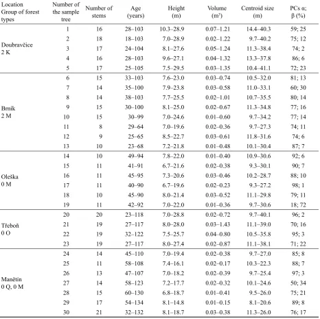
Table 1. Characteristics of the examined material

Location Group of forest types

Number of the sample

tree

Number of

stems (years)Age Height (m) Volume (m3₎ Centroid size _(m) PCs α; _{β (%)}

Doubravčice 2 K

1 16 28–103 10.3–28.9 0.07–1.21 14.4–40.3 59; 25

2 18 18–103 7.0–28.9 0.02–1.22 9.7–40.2 75; 12

3 17 24–104 8.1–27.6 0.05–1.24 11.3–38.4 74; 2

4 16 28–103 9.6–27.1 0.04–1.32 13.3–37.8 86; 6

5 17 25–105 7.5–29.5 0.03–1.35 10.4–41.1 72; 23

Brník 2 M

6 15 33–103 7.6–23.0 0.03–0.74 10.5–32.0 81; 13

7 14 35–100 7.9–23.8 0.03–0.58 11.0–33.1 60; 30

8 14 38–103 7.7–25.5 0.02–1.01 10.7–35.5 80; 14

9 15 30–100 8.1–25.0 0.02–0.67 11.3–34.8 77; 16

10 15 30–99 7.0–24.6 0.01–0.60 9.7–34.2 77; 14

11 8 29–64 7.0–19.6 0.02–0.36 9.7–27.3 74; 11

12 9 25–65 8.5–22.7 0.03–0.61 11.8–31.6 74; 6

13 10 23–68 7.2–21.8 0.01–0.48 10.1–30.4 87; 7

Oleška 0 M

14 10 49–94 7.8–22.0 0.01–0.40 10.9–30.6 92; 6

15 11 41–91 6.7–21.6 0.02–0.38 9.3–30.1 90; 7

16 11 45–95 7.3–20.6 0.03–0.46 10.2–28.7 88; 10

17 11 40–90 6.7–19.6 0.02–0.23 9.3–27.2 98; 1

18 10 45–90 8.0–21.4 0.03–0.52 11.1–29.8 79; 11

19 11 42–92 7.0–22.0 0.01–0.36 9.7–30.6 18; 72

Třeboň 0 O

20 20 23–118 7.0–28.8 0.02–0.72 9.7–40.1 96; 2

21 19 27–117 8.0–28.0 0.03–1.43 11.1–39.0 70; 16

22 19 32–122 7.5–25.7 0.04–0.80 10.5–35.8 95; 3

23 19 27–117 8.0–27.4 0.02–0.87 11.1–38.1 71; 22

Manětín 0 Q, 0 M

24 14 45–110 7.0–19.4 0.02–0.38 9.7–27.0 85; 8

25 11 58–108 7.4–16.1 0.02–0.17 10.3–22.3 88; 7

26 13 47–107 7.0–18.2 0.02–0.39 9.7–25.4 97; 3

27 14 58–123 7.2–17.7 0.02–0.32 10.1–24.6 50; 34

28 15 60–130 6.8–18.7 0.01–0.41 9.5–26.0 75; 21

29 17 54–134 8.1–14.8 0.01–0.15 8.1–20.6 89; 8

30 21 32–132 8.1–18.7 0.03–0.38 11.3–26.0 76; 17

6 (M + 1) n1 – 1 n2 – 1 n1 + n2 – 2 

The null hypothesis is rejected if M_B ≥ χ2

F_stat is evaluated for B random permutations T₁,...,T_B. The ranking r of the observed test statistic T_abs is then used to give the p-value of the test:

r – 1

p-value = 1 – –––––

B + 1

For each pair of locations, 1,000 random permutations were performed.

Variability

The principal component analysis was used to analyse the shape variability. The sample variance-covariance matrix of tangent coordinates was calculated for the tree set:

1 – –

S = ––– (v_i – v) (v_i – v)T

n

1 where v = ––– ∑v_i

n

The orthogonal eigenvectors of S, denoted by χ_j are the

principal components of S with corresponding

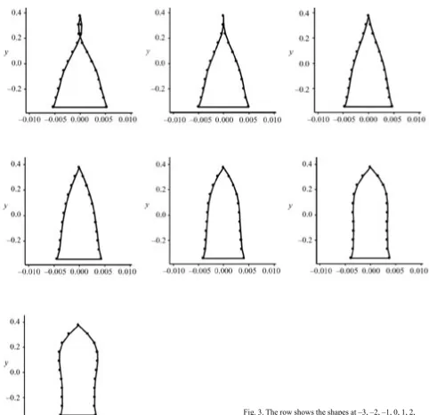
eigenval-ues λ1 ≥ λ2 ≥ ... ≥ λj ≥ 0, where j = min (n – 1, M). Fig. 3. The row shows the shapes at –3, –2, –1, 0, 1, 2, 3, standard deviations along the second PC (β)

Table 2. Eigenvalues of the variance-covariance matrix from the set of Scots pine stems and proportional expression of variability explained by them

Eigenvalue λj .10–3

p

λj l ∑ λj . 100 (%) j = 1

λ1 1.691 87

λ2 0.496 8

The principal component (PC) score for the i-th

indi-vidual on the j-th principal component is given by

s_ij = χT j (vi – v)

The standardized PC scores are _s

ij c_ij = –––– √λij

RESULTS AND DISCUSSION

As can be seen in Table 2, the first three principal compo-nents (PC) include 98% of all variability. Out of it, the first two cover 95% of the variability. Figs. 2 and 3 show a series of stem shapes evaluated in accordance with the first two PCs. In each row, the middle plot is the mean shape. First PC is labelled (α). Similarly like in spruce, see KŘEPELAet al. (2001) and KŘEPELA (2002), the first PC is symmetric, it points across the vertical stem axis. The second PC is asym-metric. It has an opposite direction in the bottom section (up to 4/10 of the stem height) and top section of the stem. This PC is labelled (β) and it has not occurred at spruce amongst the first three principal components in the cited works of the authors, nor has the third PC shown in Table 2 occurred at spruce. It is not caused by the effect of buttresses or hyper-trophy of the lower part of the stem. Representation of the first two PCs for each sample tree is shown in Table 1. Full stem analysis of sample tree No. 26 between the age of 47 and 107 years is presented in Fig. 4. Here, considerable increment in the last five-year period is noticeable. Figs. 5 and 6 show shape changes in sample tree No. 26. In the age group of 47–77 years, we see only slight changes of PC (α). In the age group of 77–107 years, the stem steadily widens in its full length. See also diagrammatized Fig. 1, where the triangle basis in 1/10 of the stem has widened. In the age group of 102–107 years, the examined stem had a consider-able height increment. The increment was not accompanied by a corresponding diameter increment. It means that PC (β) changed considerably.

Mean shape of Scots pine within the Třeboň location dif-fered from those in all other locations, except the Oleška location. The Manětín location differed from the Brník and Doubravčice locations. In the other location pairs, the test did not show any statistically significant difference.

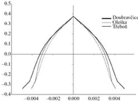
Fig. 7 shows the full Procrustes mean shapes of Scots pine in the Doubravčice, Oleška and Třeboň locations. We see a noticeable difference of the Třeboň location. It is ex-plained by the second PC. Scots pine stems in the Třeboň location are narrow in the lower part of the stem and wide

Fig. 4. Full stem analysis of the sample tree No. 26

Fig. 5. Stem shapes of the sample tree No. 26 expressed by full Procrustes coordinates

Fig. 6.The standardized PC scores of individual stems of the sample tree No. 26

in the top part of the stem. This difference is also evident in comparison with the Brník and Manětín locations, whose mean shapes were not included in the figure.

CONCLUSIONS

Shape variability analysis performed by the method of principal components for all 430 stems of Scots pine in five locations showed that 95% of variability can be explained by the first two PCs. The first PC explains 87% of variability and has the identical graphic effect as the most prominent PC at spruce – see earlier articles and studies of the authors. Within 98% of shape variability, the effect of buttresses was not recorded, in comparison with spruce. The second PC explains 8% variability. It is noticeable at Scots pine in Třeboň location. Together with the Manětín location, the Třeboň location shows the most marked difference from the other locations. The difference cannot be caused by the social position of the tree within the stand, as most of the trees were dominant, or, exceptionally, co-dominant, nor is it influenced by the age. It can point, though, to another ecotype of the tree species.

References

DRYDEN I.L., MARDIA K.V., 1998. Statistical shape analysis. Chichester, New York, Weinheim, Brisbane, Singapore, To-ronto, John Wiley & Sons: 345.

DRYDEN I. L., 2000. Statistical shape routines. University of Nottingham. http://www.maths.nottingham.ac.uk/personal/ild/ Shape-R/Shape-R.html.

HAVRÁNEK T., 1993. Statistika pro biologické a lékařské vědy. Praha, Academia: 478.

KŘEPELA M., 2002. Point distribution form model for spruce stems (Picea abies [L.] Karst.). J. For. Sci., 48: 150–155. KŘEPELA M., SEQUENS J., ZAHRADNÍK D., 2001.

Dendro-metric evaluation of stand structure and stem forms on Norway spruce (Picea abies [L.] Karst.) sample plots Doubravčice 1, 2, 3. J. For. Sci., 47: 419–427.

MARDIA K.V., KENT J.T., BIBBY J.M., 1979. Multivariate Analysis. London, New York, Toronto, Sydney, San Francisco, Academic Press: 521.

SEQUENS J., 1985. Ověření bonitního vějíře borových RT ČSSR 1980 na podkladě rozboru výškového růstu této dřeviny. Praha, VŠZ, Kostelec nad Č. lesy: 38.

SEQUENS J.,1994. Bonitní vějíř a trendy výškového růstu borovice. Lesnictví-Forestry, 40: 550–556.

Received for publication November 10, 2003 Accepted after corrections January 28, 2004

Fig. 7. Full Procrustes mean shapes of Scots pine in Doubravčice, Oleška and Třeboň locations

Příspěvek k poznání tvaru kmene borovice lesní (

Pinus sylvestris

L.)

M. KŘEPELA, J. SEQUENS, D. ZAHRADNÍK

Fakulta lesnická a environmentální, Česká zemědělská univerzita v Praze, Praha, Česká republika

Procrus-Tvar kmene borovice lesní byl zkoumán na třiceti vzornících z pěti lokalit na území ČR. Z těchto 30 vzor-níků bylo metodou plné analýzy zrekonstruováno celkem 430 kmenů (tab. 1). Na tyto kmeny bylo umístěno celkem 21 hraničních bodů – první dvojice do 0,3 m a dále výšky stoupaly po 1/10 výšky kmene až po vrchol. Jednotlivé výšky a tloušťky vytvářejí konfigurační matice a z nich byly metodou zobecněné Procrustovy analýzy (GPA) odhadnuty plné Procrustovy tvarové souřadnice a plný Procrustův tvarový průměr pro všechny kmeny, jednot-livé lokality a vzorníky. Metoda GPA byla zjednodušeně vysvětlena na metodě běžné Procrustovy analýzy (OPA) pro dva trojúhelníky, které zjednodušeně reprezentují tvar dvou kmenů starých 102 a 57 let v rámci vzorníku č. 26. Na obr. 1 je patrná širší základna kmene o stáří 102 let. Základny byly umístěny do 1/10 výšky kmene.

Pro střední tvarové vektory jednotlivých lokalit, odhadnuté z tangentových souřadnic [ty jsou získány z plných Procrustových souřadnic jejich převedením

do lineární tangentové sféry podle postupu DRYDENA

a MARDII (1998)], byly provedeny Hotellingovy T2 _testy rovnosti středních tvarových vektorů. Předtím byl pro-veden test homogenity variančně-kovariančních matic.

Test se nazývá Boxův M test [Box (1949) in MARDIA

et al. (1979) a in HAVRÁNEK (1993)]. Shoda

varianč-ně-kovariančních matic nebyla prokázána, proto byl proveden neparametrický Monte Carlo test. Pro každou dvojici lokalit bylo provedeno celkem 1 000 náhodných permutací. Tvarový průměr borovic z lokality Třeboň se odlišoval od všech ostatních lokalit s výjimkou lokality Oleška. Lokalita Manětín se odlišovala od lokality Brník a Doubravčice. V ostatních dvojicích lokalit neprokázal

použitý test na hladině významnosti α = 0,05 statisticky

významný rozdíl. Na obr. 7 jsou zachyceny plné Procrus-tovy průměrné tvary borovic pro lokality Doubravčice,

Oleška a Třeboň. Vidíme zde nápadnou odlišnost lokality Třeboň. Tato odlišnost je vysvětlena hlavní

komponen-tou (β). Kmeny třeboňské borovice jsou úzké ve spodní

části kmene a široké v horní části kmene. Tato odlišnost je patrná i vzhledem k lokalitám Brník a Manětín, jejichž tvarové průměry nebyly pro přehlednost do obrázku za-řazeny.

Variabilita byla zkoumána metodou hlavních kompo-nent. V souboru 430 kmenů první tři hlavní komponenty vysvětlují 98 % variability. Obr. 2 a 3 znázorňují grafický efekt prvních dvou hlavních komponent. První hlavní

komponenta byla označena (α). Obdobně jako u smrku

– viz KŘEPELA et al. (2001) a KŘEPELA (2002) – je její

grafický efekt symetrický podél svislé osy kmene. Druhá hlavní komponenta je asymetrická. Její grafický efekt má opačný směr ve spodní (do 4/10 výšky kmene) a horní

části kmene. Tato hlavní komponenta byla označena (β).

Tato hlavní komponenta se v citovaných pracích autorů tohoto článku u smrku nevyskytovala mezi prvními tře-mi hlavnítře-mi komponentatře-mi. Ani v tab. 2 uvedená třetí hlavní komponenta se u smrku nevyskytovala. Nejde o efekt kořenových náběhů či zbytnění spodní části kmene. Zastoupení prvních dvou hlavních komponent pro jednotlivé vzorníky zachycuje tab. 1. Plná kmenová analýza vzorníku č. 26 mezi stářím 47 až 107 let je za-chycena na obr. 4. Zde je nápadný velký výškový přírůst v poslední pětileté periodě. Na obr. 5 a 6 jsou zachyceny tvarové změny vzorníku č. 26. V periodě 47–77 let

do-chází u PC (α) jen k malým změnám. V periodě 77 až

107 let dochází k rovnoměrnému rozšiřování kmene po celé jeho délce. Mezi stářím 102–107 let došlo u sle-dovaného kmene k velkému výškovému přírůstu. Tento přírůst nebyl doplněn odpovídajícím přírůstem tloušť-kovým. Došlo tedy k velké změně u hlavní komponenty (β).

tovy tangentové souřadnice zkoumána variabilita metodou hlavních komponent. Dvě nejdůležitější hlavní komponenty byly gra-ficky znázorněny a popsány. Dále byly provedeny statistické testy mezi středními tvarovými vektory pro jednotlivé lokality.

Klíčová slova: borovice lesní (Pinus sylvestris L.); tvar kmene; Procrustova analýza; analýza hlavních komponent

Corresponding author:

Doc. Ing. JOSEF SEQUENS, CSc., Česká zemědělská univerzita v Praze, Fakulta lesnická a environmentální, 165 21 Praha 6-Suchdol, Česká republika