An investigation into the geometric parameters affecting field uniformity in four pole magnetisers

An Investigation into the Geometric

Parameters Affecting Field Uniformity in

Four Pole Magnetisers

James Borg Bartolo1, Piotr Klimczyk2, Kai Tiwisina2, Patrick Denke2, Stefan Siebert2, Christopher Gerada1

1_{University of Nottingham, NG72RD Nottingham UK,}

2_{Dr. Brockhaus Messstechnik GmbH & Co. KG, D-58507 Lüdenscheid Germany}

([email protected])

Abstract. In recent years, the field-metric method for measuring the joule losses set up in an electrical steel laminate when

subjected to a rotating field has gained popularity. The ideal geometry of the magnetiser required to set up such a field is still however the subject of much debate. The work presented in this paper aims at providing some useful guidelines which might be considered when undertaking the construction of the simplest of such magnetizing setups having four salient poles excited by a two phase system and using a square sample. A 3D model for this rotational power loss tester was simulated for different pole geometries with the induction uniformity being assessed for every alteration.

1. Introduction

In a bid to reduce cost and weight, the demand for high speed, high power density electrical machines operating at high levels of efficiency has over the past decade seen an unprecedented increase. To enable such an increase in power density an increase in both fundamental supply frequency and current loading is often required. This coupled with novel stator/winding geometries expose the constituent magnetic materials of the machine to harmonic rich excitation frequencies at high field intensity values.

The design of the required cooling regimes for such novel designs is closely linked to the correct estimation of the incurred iron losses due to both spatially pulsating and rotating fields. A general consensus on the measurement of pulsating/ alternating losses in electrical steel has led to standards such as the IEC 60404 being widely adopted. Unfortunately this is not the case for the measuring of iron losses due to spatially rotating fields. A number of methods have been proposed for the job, [1], [2] with a limited agreement being achieved on the reported loss values, as reported in [3].

Over the past years the field-metric approach, based on the Poynting’s theoremdescription of the rotational loss problem, as given in [4], has gained preference. A number of different magnetiser geometries, [5], [6], were described as possible solutions to achieve induction uniformity. The simplicity in design of the two-phase four-pole geometry, however, allows for high precision in manufacturing and sample location.

The work presented in this paper is based on such a commercially available two-phase, four-pole test setup and aims at providing an insight into the affects of various pole geometries on the induction, level and quality, within the test sample. Such work aims to contribute to knowledge already presented in [5, 7, 8] by further investigating the affect of the introduction of a pole side taper, and magnetiser assembly imperfections such as pole-yoke air gaps. The presented conclusions are based on an induction uniformity analysis performed on field maps obtained via 3D finite element simulations.

2. Model geometry and simulation setup

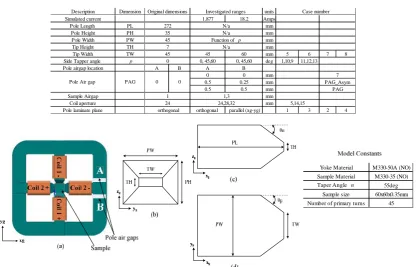
To cater for the affects of pole tapering, pole-yoke air gaps and the proper location of the sample plane (x-y) with respect to the pole tip, in the z dimension, a 3D model of the magnetising yoke was setup as shown in Figure1(a) with the salient pole parameters shown in Figures.1.(b, c, d) for different projections. The optimal

dimensions for the pole taper ‘ϑn’, tip height ‘TH’ and sample size were discussed in [8],[5] and empirically

deduced via a number of built tester iterates. In this study, such parameters are therefore considered as constant as detailed in Figure 1 and Table 1. The varied dimensions are detailed section 4 along with the results obtained for the figures of merit, (section 3), obtained for each case.

Due to computational requirements and for the purpose of such geometric optimisation it was considered sufficient to analyse the field maps, B(x,y,z), taken from the centre plane, of the sample for 1 time instant, using a 3D finite element solver, at this stage the variation in field distribution along the sample’s depth was not evaluated. The sample material was modelled as isotropic with a non-linear BH curve, typical for M330-35A

system having 273100 nodes and a liner interpolating function was used to evaluate field quantities at required sampling points. In the results which follow, coil 2 (ref. Figure 1) is energised inducing a flux along the x-axis.

Table 1

Investigated variations in Pole Geometry, note cases 5and 7 use the original dimension set

Description Dimension units

Simulated current 1.877 18.2 Amps

Pole Length PL mm

Pole Height PH mm

Pole Width PW mm

Tip Height TH mm

Tip Width TW 45 60 mm 5 6 7 8

Side Tapper angle θp 0, 45,60 0, 45,60 deg 1,10,9 11,12,13

Pole airgap location A B A B

0 0 mm

0.5 0.25 mm

0.5 0.5 mm

Sample Airgap mm

Coil aperture mm

Pole laminate plane orthogonal parallel (xg-yg) 1 3 2 4 Investigated ranges

N/a Function ofθp

N/a N/a Original dimensions

272 35 45 7 45 0

1 24 orthogonal

Case number

24,28,32

PAG Pole Air gap PAG 0 0

7 PAG_Asym

5,14,15 1,3

Yoke Material M330-50A (NO)

Sample Material M330-35 (NO) Taper Angleθn 55deg

Sample size 60x60x0.35mm

Number of primary turns 45

Figure 1 Magnetising yoke geometry in full plan view including the introduction of the parasitic air gaps at the pole-yoke interface (a).frontal projection of a pole tip (b), side elevation of a pole tip (c) and plan view of a pole tip (d).

3. Criteria for assessing induction uniformity

The proposed variations to the pole geometry were assessed on the basis of their affect on the induction uniformity within the sample. Such uniformity was assessed globally, using a rate of change criterion, whilst

locally; the deviation of edge and corner induction values from the sample’s meaninduction value, evaluated in the area enclosed by the measuring coils, was employed.

3.1 The mean rate-of-change criterion

Using the coordinate system defined in Figure 2, and considering the condition, in which only coil 2 is energised, the flux density variation brought about by the flux traversing the sample in the yg-zgplane is of interest. The resulting spatial variation in induction magnitude at the centre plane coordinate zmid, |B|(x, y, zmid), was extracted using a smoothing function into a square matrix, B[i,j]. This matrix, obtained by discretizing the

sample space using n x m points, would have its column vectors Bx, of size [n x1], represent the field variation

along the discretised x-axis, xg[i] and row vectors By, of size [1x m], represent the field variation along the discretised y-axis yg[j] of the sample, for i=1,2,...n, and j=1,2,...m.

To evaluate uniformity in the resulting discrete spatial domain, the finite difference between the By values

(difference along the ygdirection) at each discrete volume defined by the increment in the x-direction xg[i], must

be evaluated. The more uniform the distribution of B within the particular yg-zgplane of interest; the smaller the

finite difference values obtained with respect to yg. A difference matrix is thus formed having n row vectors

each with index, i, representing the finite difference vectors at each location xg[i].This concept is illustrated in

Figure 3, in which the finite-difference variations along the yg[j]-dimension at two xg[i] locations, i=1, (flux entry point) and i=10 (at 6mm within the sample) are shown, for a 100 point discretisation of the coordinate space.

,... 2 , 1 ; ,... 2 , 1 ] 1 , [ ] , [ 2 ] 1 , [ ] 1 , [ ] 1 , [ ] 2 , [ 1 ] [ 1 2 m j n i y m i B m i B y j i B j i B y i B i B m i B m j

y   

                 



Where: i denotes the index along the column vector whilst j is the index along the row vector.

10 20 30 40 50 60 70 80 90 100

-0.2 -0.15 -0.1 -0.05 0 0.05 0.1 0.15 0.2 j  B /  y

|i=1, i=

10 i=1 i=10 00157 . 0 ] 1 [  By

000223 . 0 ] 10 [  By

Figure 2 (a) Reference system used, (b) Variation of finite differences against sample number along the ygdirection Thus in order to obtain a figure of merit which expresses the field uniformity across the whole sample, the

mean of the vector expressed in equation (1) was evaluated and denoted by,

M

Evaluating this mean will give an indication of how the induction parallel to the excited yoke tip, (in this case parallel to the y-direction, will vary as one moves from one pole to the next. The magnitude of such a mean and resulting standard deviation, are therefore used as the primary criteria to assess the field uniformity in the sample. Smaller values for both figures of merit reflect a more uniform field.

3.2 The Induction deviation criteria

The resulting deviation from the mean sample induction at the sample edges and corners (as defined in Figure.2) was used as a metric for the comparison of local field uniformity. The mean sample induction value was evaluated over the area enclosed by the measuring coils at the centre of the sample. The deviation at the

sample’s edge was computed using the first and last row vectors of the induction matrix as expressed in equation (2b). m j n i B B j i ca ca

rc ; 1, ; 1,

] ,

[  _{ }

B

 (2a) [] ; i 1,n B B i ca ca e   By

 (2b) i n j m

B B j i y x ca ca

m ; 1,.. ; 1,...

] , [ ) ,

( B   

 (2c)

Where: εrcis the deviation at the sample corners, εeis the deviation at the sample edges, B[i,j] is the induction matrix, By[i] is the induction matrix and Bcais the induction level averaged over the coil aperture area. The

resulting deviation or ‘error’surface is also computed,εm(x,y), for each case, illustrating the spatial deviation in

the measured induction magnitude at a given location when compared to the sample’s mean induction.

4. Results

The spatial mean-rate-of-change index MByxfor the investigated cases along with induction deviation at the

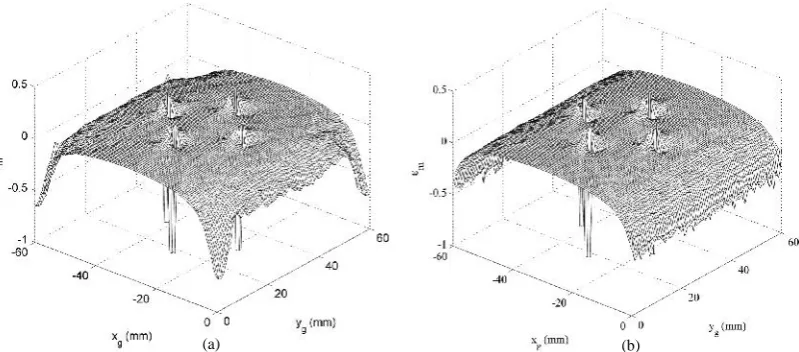
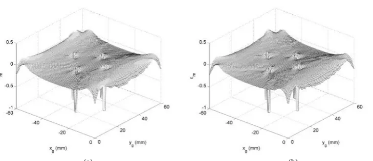
edges and corners is tabulated in Tables 2a,b. The resulting error surfaces showing the differences between the saturated and unsaturated cases pole tip affects and the inclusion of pole air gaps are given in Figures 3 to 5.

Table 2a

Summary of the obtained results

Case number

Laminate

orientation Tip width Side taper Coil aperture

Sample air-gap

Excitation

current Bca |MByx| Standard Deviation for MBy x

Deviation at sample Edge A Deviation at sample Edge B

A B εe εe 1 2 3 4

mm Deg mm mm mm mm Amps Tesla

1 Orthogonal 45 0 24 3 0 0 1.877 0.82351 9.06E-06 9.17E-05 -0.5331 -0.5364 -0.6006 -0.6165 -0.5952 -0.6286

2 Parallel 45 0 24 3 0 0 1.877 0.83557 6.63E-06 9.74E-05 -0.5329 -0.5351 -0.5999 -0.6152 -0.5942 -0.6261

3 Orthogonal 45 0 24 3 0 0 18.2 1.7557 1.36E-05 0.000175 -0.0687 -0.0689 -0.1130 -0.1325 -0.1366 -0.1412

4 Parallel 45 0 24 3 0 0 18.2 1.7585 1.40E-05 0.000176 -0.0682 -0.0685 -0.1117 -0.1310 -0.1355 -0.1399

Table 2b

Summary of obtained results

Case number

Laminate

orientation Tip width Side taper Coil aperture

Sample air-gap

Excitation

current Bca |MByx| Standard Deviation for MBy x

Deviation at sample Edge A

Deviation at sample Edge B

A B εe εe 1 2 3 4

mm Deg mm mm mm mm Amps Tesla

5 Orthogonal 45 0 24 1 0 0 1.877 1.2283 9.07E-06 0.000217 -0.3538 -0.3631 -0.7116 -0.6890 -0.7110 -0.6915 6 Orthogonal 60 0 24 1 0 0 1.877 1.2249 5.5E-05 0.000393 -0.5154 -0.5131 -0.2725 -0.1376 -0.0836 -0.1404 7 Orthogonal 45 0 24 1 0 0 18.2 1.7756 2.15E-05 0.000255 -0.0513 -0.0460 -0.2196 -0.2399 -0.2079 -0.1977 8 Orthogonal 60 0 24 1 0 0 18.2 1.7775 8.33E-06 0.000282 -0.0554 -0.0469 0.1452 0.1523 0.1485 0.1437 1 Orthogonal 45 0 24 3 0 0 1.877 0.82351 9.06E-06 9.17E-05 -0.5331 -0.5364 -0.6006 -0.6165 -0.5952 -0.6286 9 Orthogonal 45 60 24 3 0 0 1.877 0.82864 1.43E-05 0.000102 -0.5362 -0.5371 -0.5745 -0.5838 -0.5645 -0.6063 10 Orthogonal 45 45 24 3 0 0 1.877 0.82668 2.64E-06 0.000105 -0.5313 -0.5371 -0.5535 -0.5624 -0.5443 -0.5940 11 Orthogonal 60 0 24 3 0 0 1.877 0.86037 1.09E-06 9.53E-05 -0.5189 -0.5225 -0.4190 -0.3976 -0.4144 -0.4773 12 Orthogonal 60 60 24 3 0 0 1.877 0.85311 1.11E-05 0.000123 -0.5154 -0.5230 -0.4105 -0.3944 -0.4276 -0.4629 13 Orthogonal 60 45 24 3 0 0 1.877 0.83566 2.57E-05 0.000142 -0.5163 -0.5246 -0.4156 -0.3520 -0.4033 -0.4632 5* Orthogonal 45 0 24 1 0 0 1.877 1.2283 2.44E-03 0.000217 -0.3538 -0.3631 -0.7116 -0.6890 -0.7110 -0.6915 14* Orthogonal 45 0 28 1 0 0 1.877 1.1549 2.02E-03 0.000159 -0.5005 -0.5017 -0.7155 -0.7346 -0.7310 -0.7295 15* Orthogonal 45 0 32 1 0 0 1.877 1.1557 1.69E-03 0.000161 -0.5063 -0.5023 -0.7161 -0.7347 -0.7299 -0.7297 7 Orthogonal 45 0 24 1 0 0 18.2 1.7756 2.15E-05 0.000255 -0.0513 -0.0460 -0.2196 -0.2399 -0.2079 -0.1977 PAG Parallel 45 0 24 1 0.5 0.5 18.2 1.7776 5.30E-05 0.000382 -0.0406 -0.0452 -0.2102 -0.2340 -0.1684 -0.2144 PAG_asym Parallel 45 0 24 1 0.5 0.25 18.2 1.7782 4.82E-05 0.000365 -0.0404 -0.0455 -0.2082 -0.2343 -0.1631 -0.2174 Deviation at the sample cornersεrc

Pole air-gaps

*Note for Samples 5, 14 and 15 the uniformity values for the sample regions enclosed by the threaded B-coils were considered

Figure 3 Surface plot showing the deviation in sample induction from the mean value, (a) for case 1 with pole laminates orthogonal to the sample plane and Bca=0.82T, (b) case 3 with pole laminates orthogonal to the sample plane and Bca=1.75T

Figure 4 Surface plot showing the deviation in sample induction from the mean value for, (a) case 5 with tip width at 45mm and Bca=1.23T, (b) case 6 with tip width equal to sample width and Bca=1.22T

(a) (b)

Figure 5 Surface plot showing the deviation in sample induction from the mean value for (a) case 7 having a tip width of 45mm, no pole air-gaps and Bca=1.77T, (b) case PAG, with tip width at 45mm, symmetric pole air gaps and Bca=1.77T

5. Conclusion

By considering the Mean rate of change criterion, MBxy, and the mean induction deviation criteria, the following conclusions can be drawn flowing from the results presented above:

i) Induction uniformity is largely unaffected by the pole laminate orientation for high induction values and where the sample air gap is larger than 1mm, ref. cases 3and 4. For low induction values a parallel orientation of the pole tips will produce a more uniform field ref. cases 1 and 2

ii) For a sample air gap of 1mm a Tip width of 45mm will result in the best global induction uniformity at low induction values, however induction deviations for such geometry exceed those presented by the 60mm case at high induction values (ref. cases 5, 6, 7, and 8). If a large sample air-gap were to be considered, than the 60mm tip width provides for better uniformity ( ref. cases 1 and 11)

iii) Cases 7 and 3, confirm that a larger air gap leads to better induction uniformity, at the cost of reduced mean magnitude, with 1.77T and 1.75T respectively.

iv) From cases 1, 9,10, it can be seen that introducing a 45 degree side taper can help uniformity, ( ref case 1 and 10) for the case in which a 45mm tip width is considered with a 3mm air gap. Otherwise such a feature does not greatly enhance uniformity, (ref cases 11, 12, 13).

v) From cases 5, 14, 15, it can be seen that the B-sensing coil aperture is critical in through-hole setups.

vi) Introducing pole air gaps reduces the mean induction value; this however, is also accompanied by a reduction in uniformity. Also it should be noted that for cases PAG, PAG_asym, corner 3, ( lying opposite to the introduced gaps), exhibits the lowest deviation from the mean induction level due to the experienced increased flux leakage as expected.

6.

References

[1] Guo,Y., Zhu J.G., Zhong J.,LuH., Jin J.X., Measurement and Modeling of Rotational Core Losses of Soft Magnetic

Materials Used in Electrical Machines: A Review. IEEE Trans. on Magnetics, 2008. 44(2).

[2] Sievert, J. D., Two-dimensional magnetic measurements – history and achievements of the workshop. Przeglad

Elektrotechniczny (Electrical review), 2011. 87 (9b).

[3] Sievert, J.D., Ahlers H, Birkfeld M, et al, European intercomparison of measurements of rotational power loss in

electrical sheet steel. Journal of Magnetism and Magnetic Materials, 1996. 160.

[4] Brix,W., Hempel K. A., Schreoder W, Method for the measurement of rotational power loss and related properties in

electrical steel sheets. IEEE Trans. on Magnetics, 1982. 18(6).

[5] Bottauscio, O., Chiampi M, Fiorillo F, Manzin A. Space and Time Distribution of Magnetic Field in 2D Magnetizers. in

8th International Workshop on One-and Two-Dimensional Magnetic Measurement and Testing 2005. Belgium: Polish

Electrotechnical review.

[6] Alatawneh, N., Pillay P. Design of a Novel test Fixture to Measure Rotational Core Losses in Machine Laminations. 2011. IEEE.

[7] Pfutzner, H., Krismanic G., Yamaguchi H., Leiss E., Chiang WC., A study on possible sources of errors of loss

measurement under rotational magnetization. Przeglad Elektrotechniczny (Electrical review), 2007. 83(4).

[8] Enokizono, M., Sievert J D, Numerical Analysis of Accuracy of Roataional Magnetic Loss Measurement Apparatus. IEEE Trans. on Magnetics in Japan, 1990. 5 (9).