Context dependent reduction in somatic condition of wild Atlantic salmon infested with sea lice

1

Supplement:

Context-dependent reduction in

somatic condition of wild Atlantic

salmon infested with sea lice

Roman Susdorf1,2_{, Nabeil K.G. Salama}2_{, Christopher D. Todd}3_{, Robert J. Hillman}4_{, Paul Elsmere}4 _and

David Lusseau1

1 _{University of Aberdeen, School of Biological Sciences, Tillydrone Avenue, Aberdeen AB24 2TZ, UK}

2 _{Marine Scotland Science, Marine Laboratory, 375 Victoria Road, Aberdeen AB11 9DB, UK}

3_{Scottish Oceans Institute, School of Biology, University of St Andrews, St Andrews, Fife KY16 8LB, UK} 4_{Environment Agency, Sir John Moore House, Victoria Square, Bodmin, PL31 1EB, UK}

2

Supplement 1: Sample size (Tables S1 & S2)

Table S1: Sample size for one-sea-winter (1SW) and multi-sea-winter (MSW) salmon, for each site (Strathy Point (SP), North Esk (NE), Tamar (TA)) in each year used for the determination of a body condition index K (weight at length).

*in Tamar each year was adjusted to match the cohort run-timing (mid March to mid March next year)

SP

NE

TA*

1SW MSW 1SW MSW 1SW MSW

1999 39 -

2000 41 -

2001 43 - 929 487

2002 53 - 1437 731

2003 63 - 1314 806 70 102

2004 62 - 466 134

2005 59 - 127 126

2006 69 - 440 131

2007 62 - 405 69

2008 166 147

2009 223 139

2010 843 172

2011 341 212

2012 116 110

2013 171 184

2014

2015 182 91

2016 200 90

All 491 - 3680 2024 3750 1707

Table S2: Sample size for each component (1SW or MSW, female (F), male (M)) in each site with known infestation density D used for the assessment of a potential effect from sea lice on condition K.

Tamar

North Esk

1SW MSW Male Female

Season

t

F M F M Month m 2001 2002 2003 2001 2002 2003

1 0 0 184 60 Apr/May 72 121 89 101 162 101

2 286 128 378 249 June 70 52 95 82 82 106

3 979 633 129 66 July 105 62 54 123 53 70

4 279 278 54 30 August 91 99 42 125 78 63

Sum 1544 1039 745 405 Sum 338 334 280 431 375 340

Strathy Point

1SW Month 1999 2000 2001 2002 2003 2004 2005 2006 2007 Sum

3

Supplement 2: Body Condition index

K

(Figure S1)

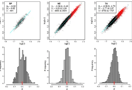
Figure S1: Top: Length-weight relationship (LWR, in cm and kg, both log10-transformed) for 491 1SW at Strathy Point (SP, left), 3680 1SW and 2024 MSW in North Esk (NE, centre), and 3750 1SW and 1707 MSW in Tamar (TA, right) according to Table S1. Each regression is described by intercept and slope parameters 𝛽0 and 𝛽1, whereas the LWR was obtained for

each sea age class individually (regression line shown in solid (1SW) or dashed (MSW)). The residuals of each linear model are used as individual body condition index K.

The intercept and slope parameters 𝛽0 and 𝛽1 of the linear model for each catchment and sea age are -5.02±0.11 and

3.02±0.06 (SP, 1SW), -5.36±0.03 and 3.23±0.02 (NE, 1SW), -5.48±0.04 and 3.28±0.02 (NE, MSW), as well as -4.56±0.04 and 2.77±0.02 (TA, 1SW), and -4.73±0.07 and 2.87±0.04 (TA, MSW). The coefficient of determination R2 _{for the} relationship between log10-transformed w and log10-transformed 𝑙is 0.82 (SP, 1SW), 0.91 (NE, 1SW), 0.92 (NE, MSW), 0.8 (TA, 1SW) and 0.77 (TA, MSW).

4

Supplement 3: Determination of sea age in North Esk (NE)

and Tamar (TA)

A.

North Esk (Figure S2+S3)

The North Esk (NE) sample consisted of 1SW (n=3677), 2SW (n=2000), 3SW (n=13), and 14 (out of overall 5704) individuals with missing sea age (𝑎) information (Figure S3). As preliminary analysis revealed that 𝑎 should be considered as covariate to describe a potential effect from sea lice on host condition K, missing 𝑎 values in the NE sample were determined in two steps using a mixture model.

Step 1: manual determination

Beforehand, the data were treated: as the weight and length of 3SW individuals is not readily distinguishable from 2SW, both age-classes were compiled into a single category: multi sea-winter (MSW) fish. Then the length 𝑙 density distribution (kernel) for each month 𝑚, year 𝑦, and sex 𝑠 was used to manually assign a specific length-threshold (near the lowest density (y-axis) between the two density peaks) which is assumed to split 1SW from MSW. Accordingly, all 5704 individuals were preliminary clustered into 2 components representing 1SW (all fish below the 𝑚-, 𝑦-, and 𝑠-specific length-threshold) and MSW (all fish above) (Figure S2). Here, 𝑙 was chosen over weight 𝑤 as it is a slightly better predictor of sea-age (adjusted R2 _{of 0.85 vs 0.83, both p≈0). A comparison with known}

sea age values resulted in an overlap of 98 %, validating the accuracy of this method. However, under the underlying assumption the lengths of the two sea age classes in each 𝑚, 𝑦, and for each 𝑠 are strictly separated and not allowed to overlap, which is inappropriate. Furthermore, this coarse approach is prone to biases with regards to the chosen length-thresholds. Nevertheless, it provides an initial probability of an individual belonging to the 1SW or MSW group, which is important information required for an accurate algorithmic sea age assessment (see Step 2). These initial 𝑎 estimates were adopted in the 14 individuals missing this parameter; i.e. for the remaining 5690 fish 𝑎 as determined from scale reading was restored.

Step 2: algorithmic determination

A Gaussian mixture model with 2-components (1SW and MSW) (R-package flexmix(Leisch 2004; Grün & Leisch 2008) v.2.3-13) with length 𝑙 as response, and Day of the Year (𝑑) (numerical), year 𝑦 (categorical), and sex 𝑠 (categorical) as predictor variables (selection based on AIC) was fitted. However, this basic model performed poorly:

flexmix(formula = l ~ d + s + y, data = dt, k = 2)

prior size post>0 ratio Comp.1 0.585 3902 5486 0.711 Comp.2 0.415 1802 5704 0.316

5

AIC: 40341.83 BIC: 40428.27

A relatively small proportion of observations with non-vanishing posteriors (post>0 in model summary) is assigned to each cluster (ratio of 0.711 (1SW) and 0.316 (MSW)), suggesting a big overlap between age classes. Overall, the model predicted unrealistic sea age values and needed improvement.

Thus, actually measured (n=5690) and manually determined (n=14) 𝑎 values (from Step 1) were used to assign an initial probability of component membership for each individual in form of a two-element vector containing (osw=1, msw=0) for 1SW and (osw=0, msw=1) for MSW. This resulted in a two-column matrix with 5704 (NE sample size) rows. This by far improved the performance of the EM algorithm with observations being assigned to the corresponding cluster at a ratio of 0.83 (Comp.1=1SW) and 0.72 (Comp.2=MSW):

flexmix(formula = l ~ d + s + y, data = dt, k = 2, cluster = matrix(c(dt$o

sw, dt$msw), 5704, 2))

prior size post>0 ratio Comp.1 0.660 3755 4543 0.827 Comp.2 0.340 1949 2723 0.716

'log Lik.' -20176.74 (df=13) AIC: 40379.48 BIC: 40465.92

6 Males

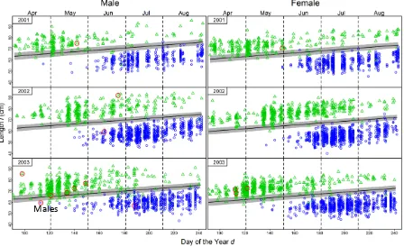
Figure S3: Day of the Year 𝑑of freshwater entry (i.e. sampling date) (x-axis) and length 𝑙 (y-axis) in cm of sampled male (left) and female (right) Atlantic salmon (n=5704) in River North Esk. 1SW are plotted as blue circles, and MSW as green triangles. In individuals with missing information on sea age (a) (highlighted in red) it was estimated using a Gaussian mixture model. All individuals below or above the grey band are assigned as 1SW or respectively MSW with a probability of over 95 %.

7

B.

Tamar (Figure S4, Table S3)

The Tamar (TA) sample consisted of 1SW (n=3595), 2SW (n=1533), 3SW (n=9), and 583 (out of overall 5720) individuals with missing sea age (𝑎) information (Figure S4). Spawning takes place around November-December each year. However, the migration of each cohort can extend from about March in one year to March the next year, with fish entering freshwater after November being most likely to postpone spawning until the subsequent spawning season. Date (Day of the Year 𝑑) in each year was adjusted to contain the whole migration period, i.e. starting in 𝑑=73 (mid March) in each year and ending in 𝑑=365+73 (mid March) (referred to as 𝑑𝑎𝑑𝑗) of the next. Year 𝑦 was adjusted according to this shift by 73 days (referred to as 𝑦_𝑎𝑑𝑗), so that the whole cohort (running from e.g. March 2011 to March 2012) was assigned a 𝑦𝑎𝑑𝑗 of 2011. Like in the NE sample, sea age 𝑎 had to be first determined manually based on length 𝑙 of each 𝑎-class at any sampling date in each year, as otherwise the EM algorithm didn’t perform appropriately.

Step 1: manual determination

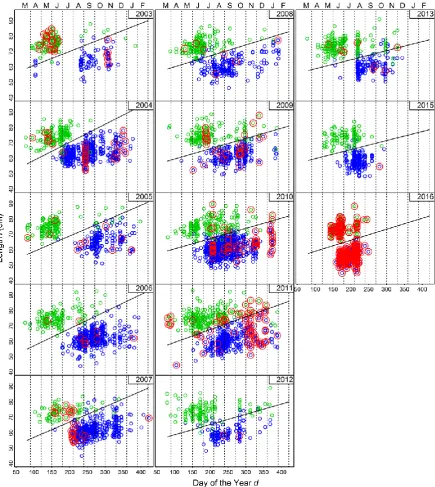
For a manual determination of 𝑎, 2SW and 3SW were compiled into a single category MSW. Then the scatterplot of length 𝑙 vs adjusted day of sampling 𝑑_𝑎𝑑𝑗 in each adjusted year 𝑦𝑎𝑑𝑗 was used to manually determine a linear model of the form 𝑙 = 𝛽0+ 𝑑𝑎𝑑𝑗𝛽1 to segregate 1SW from MSW (Figure S4). Chosen intercept and slope parameters for each year are given in Table S3. All individuals with missing 𝑎 (Figure S4, red circles) below the 𝑦_𝑎𝑑𝑗- and 𝑑_𝑎𝑑𝑗-specific length-threshold (defined by the linear model) were treated as 1SW, and all fish (with missing 𝑎) above as MSW. A comparison with known sea age values resulted in an overlap of 98 %, validating the accuracy of this method.

Step 2: algorithmic determination

Fitting a Gaussian mixture model with 2-components (1SW and MSW) (R-package flexmix(Leisch 2004; Grün & Leisch 2008) v.2.3-13) with length 𝑙 as response, and Day of the Year (𝑑𝑎𝑑𝑗) (numerical), year 𝑦_𝑎𝑑𝑗 (categorical) and Fulton’s condition index 𝐾𝐹 as predictor variables initially performed poorly:

flexmix(formula = l ~ dadj + yadj + KF, data = dt, k = 2)

prior size post>0 ratio Comp.1 0.340 2298 4115 0.558 Comp.2 0.660 3422 5720 0.598

'log Lik.' -18934 (df=33)

Table S3: Annual intercept and slope coefficients of the linear models with predictor 𝑑𝑎𝑑𝑗 (adjusted Day of the Year)

8

AIC: 37935 BIC: 38154

Only a relatively small proportion of observation with non-vanishing posteriors (0.558 and 0.598) could be assigned a sea age class. Many of the obtained sea age values were clearly wrong.

Like in NE, in an attempt to improve the mixture model, we used the actually measured (n=5137) and manually determined (n=583) 𝑎 values (from step 1) to assign an initial probability of component membership for each individual in form of a two-element vector containing (osw=1, msw=0) for 1SW and (osw=0, msw=1) for MSW. But this additional information did not resolve the poor performance of the model:

flexmix(formula = l ~ dadj + yadj + KF, data = dt, k = 2, cluster = matrix(c(dt$osw,

dt$msw), 5720, 2))

prior size post>0 ratio Comp.1 0.331 2234 4032 0.554 Comp.2 0.669 3486 5720 0.609

'log Lik.' -18929 (df=33) AIC: 37924 BIC: 38144

However, model performance was satisfying after adjusting a hyperparameter for the EM algorithm by using “hard” assignment of manually obtained 𝑎-values to clusters:

flexmix(formula = l ~ dadj + yadj + KF, data = dt, k = 2, cluster = matrix(c(dt$osw,

dt$msw), 5720, 2), control = list(classify="hard"))

prior size post>0 ratio Comp.1 0.669 3854 5176 0.745 Comp.2 0.331 1866 4457 0.419

'log Lik.' -19319 (df=33) AIC: 38703 BIC: 38923

9 Figure S4: Length 𝑙 (cm) vs sampling date 𝑑𝑎𝑑𝑗 (adjusted Day of the Year) for 1SW (blue dots) and MSW (green

dots) in each year (adjusted from March to March next year to match the salmon cohort migration time). The lines segregating 1SW from MSW were chosen manually, by applying a linear model with 𝑙as response and 𝑑𝑎𝑑𝑗as

10

Supplement 4: Final model diagnostics (Table S4-6, Figure

S5-7)

A.

Strathy Point

Table S4: Details for linear mixed effects model used to quantify the sea lice-mediated condition effect on 1SW Atlantic salmon sampled at SP (n=491, 1999-2007). Covariates used are infestation density D (mobile sea lice/kg, scaled), proportion of adult female L salmonis (θ, scaled) and sampling year (y)F _{as random intercepts.}

F

: applied as factor

Strathy Point

𝐾~ 𝐷+ θ + 𝐷𝜃 + (𝜃|𝑦)

Residuals:

Min 1Q Median 3Q Max -0.107 -0.0256 0.0015 0.0235 0.169

Random effects

Groups Name StdDev Corr y Intercept 0.02965 -0.01

𝜃 0.00777 Residual 0.03663 No of observations: 491; Groups: y=9 Fixed effects (model average)

Coefficient Estimate StdErr z-val p Intercept 0.00385 0.009793 0.392 0.695 D (scaled) -0.01046 0.001921 5.434 <0.001

𝜃 (scaled) 0.002106 0.002795 0.752 0.452

𝐷𝜃 -0.001718 0.002106 0.815 0.415

Marginal R-squared: 0.047 (fixed effects only)

Conditional R-squared: 0.454 (fixed and random effects)

11

B. North Esk

Table S5: Details for averaged linear model used to quantify the effect from sea lice density D on salmon condition K in NE (n=952 male and 1146 female salmon, 2001-2003). Covariates used: infestation intensity D (mobile sea lice/kg), year of sampling (y)F_{, sex (s, male=1, female=2)}F_{, sampling month} (m)F_.

F_{: applied as factor}

North Esk

𝐾~ 𝐷+ 𝑦 + 𝑠+ 𝑚 + 𝐷𝑦 + 𝐷𝑚 + 𝐷𝑠 + 𝑦𝑚

Residuals:

Min 1Q Median 3Q Max -0.2511 -0.022 0.00099 0.0228 0.193

Coefficient Estimate Adj. StdErr t-val p Intercept -0.00823 0.003034 2.712 0.007

D 0.00161 0.000989 1.63 0.103

m6 0.00871 0.004518 1.928 0.053

m7 -0.00002 0.003925 0.005 0.999

m8 0.00810 0.003889 2.082 0.037

s2 0.007631 0.001745 4.373 <0.001

y2002 0.017882 0.003594 4.976 <0.001

y2003 -0.00331 0.00391 0.845 0.398

D:m6 -0.00024 0.000912 0.26 0.795

D:m7 -0.00226 0.001056 2.141 0.0323

D:m8 -0.00326 0.001106 2.95 0.0032

D:y2002 -0.00215 0.000908 2.368 0.0178

D:y2003 -0.00285 0.000825 3.45 <0.001

m6:y2002 -0.01026 0.00561 1.829 0.067

m7:y2002 -0.00645 0.005314 1.215 0.224

m8:y2002 -0.00132 0.00494 0.266 0.79

m6:y2003 -0.01158 0.005552 2.085 0.037

m7:y2003 0.010247 0.005549 1.847 0.065

m8:y2003 -0.00933 0.005652 1.651 0.099

Residual standard error: 0.035 Multiple R-squared: 0.105 Adjusted R-squared: 0.097 F-statistic: 13.3 on 18 or 19 and 2079 DF

p-value: < 2.2e-16

12 Figure S7: Diagnostic plots for the averaged mixed effects model (“full” (in

contrast to “subset” average)) of

condition K for 1SW salmon from River Tamar (Table S6).

C. Tamar

Table S6: Details for the averaged (“full” (in contrast to “subset”) average) linear mixed effects model on the influence of infestation D on 1SW salmon condition K in River Tamar (TA). Covariates used are sea lice density (D, lice/kg), year of sampling (y)F _{as random effect, sex (s, male=1, female=2)}F and season (t, Mar-May=1 (MSW only), Jun-Jul=2, Aug-Sep=3, Oct-Nov=4)F_. F_{: applied as factor}

Tamar 1SW

𝐾~ 𝐷+ s + t + st + Ds + Dt +(1|𝑦/𝑡)

Scaled residuals:

Min 1Q Median 3Q Max -4.72 -0.55 0.07 0.62 4.24

Random effects

Groups Name Variance StdDev t:y Intercept 0.000112 0.0106 y Intercept 0.000123 0.0111 Residual 0.001462 0.0382

No of observations: 2583; Groups: t:y=34; y=12 Fixed effects (model average)

Coefficient Estimate StdErr z-val p

(Intercept) -0.0031 0.005595 0.553 0.58

D -0.0013 0.000499 2.603 <0.01

s2 0.0088 0.00341 2.579 <0.01

t3 0.00018 0.005547 0.032 0.97

t4 -0.03111 0.006278 4.953 <0.001

s2:t3 0.00126 0.003182 0.396 0.69

s2:t4 0.00262 0.004897 0.534 0.59

D:s2 -0.000012 0.000358 0.033 0.97

D:t3 0.000037 0.000321 0.117 0.91

D:t4 0.000004 0.000349 0.013 0.99 Marginal R-squared: 0.103 (fixed effects only)

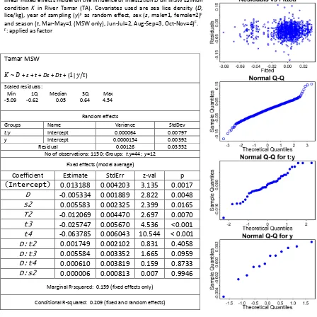
13 Figure S8: Diagnostic plots for the averaged mixed effects model (“full” (in

contrast to “subset” average)) of

condition K for MSW salmon from River Tamar (Table S7).

Table S7: Details for the averaged (“full” (in contrast to “subset”) average) linear mixed effects model on the influence of infestation D on MSW salmon condition K in River Tamar (TA). Covariates used are sea lice density (D, lice/kg), year of sampling (y)F _{as random effect, sex (s, male=1, female=2)}F and season (t, Mar-May=1 (MSW only), Jun-Jul=2, Aug-Sep=3, Oct-Nov=4)F_. F_{: applied as factor}

Tamar MSW

𝐾~ 𝐷+ s + t + Ds + Dt +(1|𝑦/𝑡)

Scaled residuals:

Min 1Q Median 3Q Max -5.09 -0.62 0.05 0.64 4.54

Random effects

Groups Name Variance StdDev t:y Intercept 0.000064 0.00797 y Intercept 0.0000154 0.00392 Residual 0.00126 0.03552

No of observations: 1150; Groups: t:y=44; y=12 Fixed effects (model average)

Coefficient Estimate StdErr z-val p

(Intercept) _{0.013188 0.004203 3.135 0.0017}

D _{-0.005334 0.001889 2.822 0.0048} s2 0.005583 0.002325 2.399 0.0165

T2 -0.012069 0.004470 2.697 0.0070

t3 -0.025747 0.005670 4.536 <0.001

t4 -0.063785 0.006043 10.544 < 0.001

D:t2 0.001749 0.002102 0.831 0.4058

D:t3 0.005584 0.003352 1.665 0.0959

D:t4 0.000610 0.003819 0.159 0.8733

D:s2 0.000006 0.000813 0.007 0.9946

Marginal R-squared: 0.159 (fixed effects only)

14

Supplement 5: Infestation levels (Figure S9)

Figure S9: