A predictive control strategy for a single phase AC AC converter

A Predictive Current Control for a

Single-Phase Matrix Converter

M. Rivera, S. Rojas

Universidad de Talca Curico, CHILE

Email: [email protected] http://www.utalca.cl

P. Wheeler

The University of Nottingham Nottingham, U.K.

Email: [email protected] http://www.nottingham.ac.uk

J. Rodriguez

Universidad Nacional Andr´es Bello

Santiago, CHILE Email: [email protected]

http://www.unab.cl

Abstract—This paper presents a finite control set model predictive current control strategy with a prediction horizon of one sampling time to control the single-phase matrix converter. The proposed current control strategy is based on a prediction calculation to select the switching states of the converter. By using a predictive cost function, the optimal switching state to be applied to the next sampling time is selected. This is done in order to obtain a good tracking of the load currents to their respective references. The feasibility of the proposed strategy is verified by simulation and experimental results, which show good dynamic and stationary performance.

NOMENCLATURE

Variable Description

vi Input voltage [𝑣𝐴 𝑣𝐵 𝑣𝐶]𝑇

ii Input current [𝑖𝐴 𝑖𝐵 𝑖𝐶]𝑇

v Load voltage 𝑣+−𝑣−

𝑖𝑜 Load current

𝐶𝑓 Input filter capacitor

I. INTRODUCTION

The matrix converter (MC) consists of an array of bidirec-tional switches, which are used to directly connect the power supply to the load without using any dc-link or large energy storage elements [1]. The most important characteristics of matrix converters are [2], [3]: 1) a simple and compact power circuit; 2) generation of load voltage with arbitrary amplitude and frequency; 3) sinusoidal input and output currents; 4) operation with unity power factor; 5) regeneration capability. These highly attractive characteristics are the reason for the tremendous interest in this topology.

The intensive research on matrix converters began with the work of Venturini and Alesina in 1980 [2]. They provided the rigorous mathematical background and introduced the name “matrix converter”, elegantly describing how the low-frequency behavior of the voltages and currents are gener-ated at the load and input. One of the biggest difficulties in the operation of this converter was the commutation of the bidirectional switches [4]. This problem has been solved by introducing intelligent and soft commutation techniques, giving new momentum to research in the area. After almost three decades of intensive research, the development of this converter is reaching industrial application [5]. In effect, at least one big manufacturer of power converters (Yaskawa) is

𝑣𝐴

𝑣𝐵

𝑣𝐶

𝑖𝐴

𝑖𝐵

𝑖𝐶

𝑖𝑜 _𝑣𝑝

𝑣𝑛

𝐶𝑓

𝑆1

𝑆2

𝑆3

𝑆4 𝑆5 𝑆6

Fig. 1. Topology of the single-phase matrix converter.

now offering a complete line of standard units for up to several megawatts and medium voltage using cascade connection. These units have rated power (and voltages) of 9-114 kVA (200 V and 400 V) for low voltage MC, and 200-6.000 kVA (3.3 kV, 6.6 kV) for medium voltage [1]. Years of continuous effort have been dedicated to the development of different modulation and control strategies that can be applied to matrix converters [4], [6]–[12].

Regarding the main applications of matrix converters there are two main approaches: (1) speed variation on fans and pumps that require strict control of harmonic distortion and on the other hand (2) applications with high mechanical inertia as centrifuges, cranes and mechanical stairs, in order to employ the regenerative capacity [1].

predict its future behavior, and, based on this prediction, the proper switching state is selected [14]. Thanks to the accurate models available for the electrical systems, the finite number of feasible commutation states of the power converters, and the fast sampling frequencies achieved with the actual digital signal processors, predictive control has emerged as one of the most effective techniques for matrix converters [15].

This paper presents a predictive current control strategy for a single-phase matrix converter. This converter is the basic cell of the converter presented in [1]. The proposed control scheme predicts the future load current behavior for each valid switching state of the converter, in terms of the measured load current and predicted load voltage. The predictions are evaluated with a cost function that minimizes the error between the predicted currents and their references at the end of each sampling time. To validate the proposed method, simulations are carried out followed by experimental results implemented in a laboratory prototype.

II. TOPOLOGY ANDMATHEMATICALMODEL OF THE

SINGLE-PHASEMATRIXCONVERTER

The mathematical model of the single-phase matrix con-verter is obtained from Fig. 1. The output voltage𝑣= [𝑣𝑝−𝑣𝑛] is obtained as a function of the converter’s switches and the input voltages v_i, as follows:

𝑣𝑝₌[ _𝑆

1 𝑆2 𝑆3 ]vi, (1)

𝑣𝑛₌[ _𝑆

4 𝑆5 𝑆6 ]vi. (2)

The input currents i_i are synthesized as a function of the

converter’s switches and the load current 𝑖𝑜:

ii=

⎡

⎣ 𝑆_𝑆1₂−₋𝑆_𝑆4₅ 𝑆3−𝑆6

⎤

⎦_𝑖𝑜. (3)

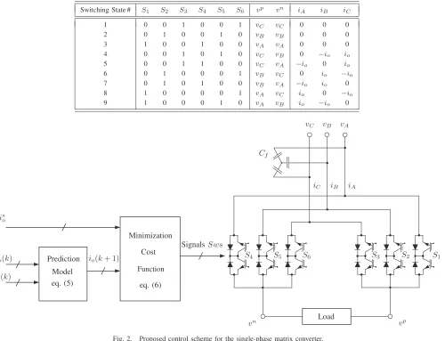
These equations correspond to the nine valid switching states of the converter, as reported in [16], and following the restrictions of no short circuits in the input and no open lines in the output. A summary of the valid switching states of the converter and the output voltage and input currents for each switching state is presented in Table I. Finally, assuming an inductive-resistive load, the following equation describes the behavior of the load:

𝑑𝑖𝑜 𝑑𝑡 =

1

𝐿𝑣− 𝑅

𝐿𝑖𝑜. (4)

III. PREDICTIVECURRENTCONTROL FOR THE

SINGLE-PHASEMATRIXCONVERTER

The control scheme for the single-phase matrix converter is represented in Fig. 2. The approach pursues the selection of the switching state of the converter that leads the output current closest to its respective reference at the end of the sampling period.

First, the control objective is determined and the variables necessary to obtain the prediction model are measured and calculated. The system model and measurements are used to predict the behavior of the variable that will be controlled in

the subsequent sampling time for each of the valid switching states. The predicted value is then used to evaluate a cost function which deals with the control objective.

After that, the valid switching state that produces the lowest value of the cost function is selected for the next sampling period. In order to compute the differential equation shown in eq. (4), the general forward-difference Euler formula is used as the derivative approximation to estimate the value of each function one sample time in the future.

A. Prediction model

The output current prediction can be obtained using a forward Euler approximation in eq. (4):

𝑖𝑜(𝑘+ 1) =𝑑1𝑣(𝑘) +𝑑2𝑖𝑜(𝑘), (5)

where, 𝑑₁ = 𝑇_𝑠/𝐿 and 𝑑₂ = 1 −𝑅𝑇_𝑠/𝐿 are constants

dependent on load parameters and the sampling time𝑇_𝑠[17].

B. Cost function

The cost function is defined in equation (6), where the error between the reference and the predicted value of the output current is considered.

𝑔(𝑘+ 1) = (𝑖∗

𝑜(𝑘+ 1)−𝑖𝑜(𝑘+ 1))2. (6)

The goal of cost function optimization is to achieve𝑔 value

close to zero. The switching state that minimizes the cost function is chosen and then applied at the next sampling instant.

Additional constraints such as current limitation and spec-trum shaping can also be included in the cost function. During

each sampling instant, the minimum value of𝑔is selected from

the 9 function values. At 𝑘𝑡ℎ instant, the algorithm selects a

switching state which would minimize the cost function at the

𝑘+ 1 instant, and then applies this optimal switching state

during the whole𝑘+ 1 period.

It is worth noting that the cost function only considers the output current. However, thanks to the absence of an energy accumulator in the matrix converter, the output current control indirectly provides an input current control. In effect, as (3) shows, the input current depends only on the commutation states and the output current. Therefore, as the output current is controlled, there is no need for internal loops to limit the input current, because the proposed control ensures that the output current will not reach any prohibitive value.

IV. SIMULATION ANDEXPERIMENTALRESULTS

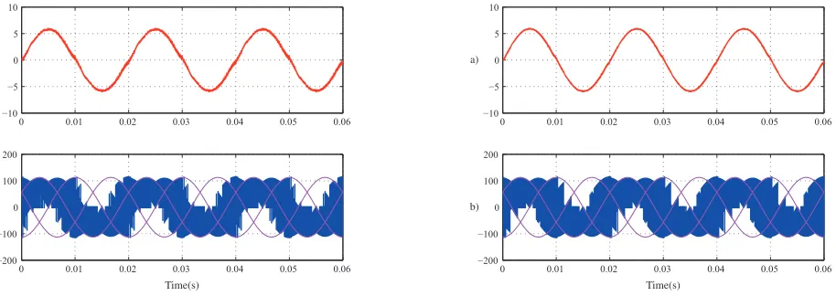
The predictive current control strategy was simulated using Gecko-Circuits with the parameters indicated in Table II and the same parameters have been used for the experimental verification. All the figures are divided in two sections: a) load current (red), b) load voltaje (blue) and source voltage (purple).

In Fig. 3 simulation are presented in steady state where

an output current amplitude of 6 Apk @𝑓_𝑜=50 Hz has been

TABLE I

FEASIBLE SWITCHING STATES OF THE SINGLE-PHASE MATRIX CONVERTER

Switching State # 𝑆₁ 𝑆₂ 𝑆₃ 𝑆₄ 𝑆₅ 𝑆₆ 𝑣𝑝 𝑣𝑛 𝑖𝐴 𝑖𝐵 𝑖𝐶

1 0 0 1 0 0 1 𝑣𝐶 𝑣𝐶 0 0 0

2 0 1 0 0 1 0 𝑣𝐵 𝑣𝐵 0 0 0

3 1 0 0 1 0 0 𝑣𝐴 𝑣𝐴 0 0 0

4 0 0 1 0 1 0 𝑣𝐶 𝑣𝐵 0 −𝑖𝑜 𝑖𝑜

5 0 0 1 1 0 0 𝑣𝐶 𝑣𝐴 −𝑖𝑜 0 𝑖𝑜

6 0 1 0 0 0 1 𝑣𝐵 𝑣𝐶 0 𝑖𝑜 −𝑖𝑜

7 0 1 0 1 0 0 𝑣𝐵 𝑣𝐴 −𝑖𝑜 𝑖𝑜 0

8 1 0 0 0 0 1 𝑣𝐴 𝑣𝐶 𝑖𝑜 0 −𝑖𝑜

9 1 0 0 0 1 0 𝑣𝐴 𝑣𝐵 𝑖𝑜 −𝑖𝑜 0

𝑣𝐴

𝑣𝐵

𝑣𝐶

𝑖𝐴

𝑖𝐵

𝑖𝐶

𝑣𝑝

𝑣𝑛

𝐶𝑓

𝑆1 𝑆2

𝑆3

𝑆4 𝑆5 𝑆6

Minimization

Cost

Function

Load

𝑖∗ 𝑜

𝑖𝑜(𝑘) 𝑖𝑜(𝑘+ 1)

𝑣(𝑘)

Signals𝑆𝑤𝑠 Prediction

Model

eq. (5) _{eq. (6)}

Fig. 2. Proposed control scheme for the single-phase matrix converter.

TABLE II SIMULATION PARAMETERS

Variables Description Value

𝑇𝑠 Sampling time 10, 20, 40 kHz

𝑉𝑠 Source voltage 56, 112 V

𝑓𝑠 Source frequency 50 Hz

𝑅 Load resistor 10Ω

𝐿 Load inductor 10 mH

are obtained for a sampling frequency of 𝑓𝑠 = 20 kHz. In

Fig. 5 and Fig. 6 are presented simulation and experimental

results for a sampling frequency of𝑓𝑠= 40 kHz, respectively.

In all these cases is observed a very good tracking of the load current to its reference under the different conditions.

One important issue that it is observed in the experimental results is the lower switching frequency in respect to the simulations which is evident in the figures. Transient analysis in both simulation and experimental have also been done. In Fig. 7 and Fig. 8 are shown simulation results for a step change in amplitude and frequency, respectively. The

amplitude change is from 3 Apk to 6 Apk @ 𝑓_𝑜 = 50 Hz

and the frequency change is from 𝑓_𝑜 = 50 Hz to 𝑓_𝑜 = 25 Hz

at a sampling frequency of𝑓_𝑠= 10 kHz. The same analysis is

done in experimental implementation as shown in Fig. 9 and Fig. 10, respectively. Again, in all these cases a very good tracking of the load current to its reference is obtained with a very fast dynamic response.

In order to assess the performance of the predictive current control scheme, two parameters are defined: the mean current tracking error and the output current THD. The percentage

mean absolute current reference tracking error%𝑒_𝑖𝑜is defined

as the absolute difference between the reference and load

currents (for 𝑚 number of samples) with respect to the rms

value of load current [18], [19]:

%𝑒𝑖𝑜 = 1

𝑚 ∑_𝑚

𝑘=0∣𝑖∗𝑜(𝑘)−𝑖𝑜(𝑘)∣

𝑟𝑚𝑠(𝑖𝑜(𝑘)) . (7)

In the case of the output current THD, it is defined as follows:

%THD=

√ 𝑠2

2+𝑠23+..+𝑠2𝑛

0 0.01 0.02 0.03 0.04 0.05 0.06 −10

−5 0 5 10

0 0.01 0.02 0.03 0.04 0.05 0.06 −200

−100 0 100 200 a)

b)

Time(s)

Fig. 3. Simulation results in steady state:𝑖_𝑜 = 6Apk;𝑓_𝑜 = 50 Hz;𝑓_𝑠 = 20 kHz;𝑣_𝑖 = 112 Vpk;

0 0.01 0.02 0.03 0.04 0.05 0.06 −10

−5 0 5 10

0 0.01 0.02 0.03 0.04 0.05 0.06 −200

−100 0 100 200 a)

b)

Time(s)

Fig. 4. Experimental results in steady state:𝑖_𝑜 = 6 Apk;𝑓_𝑜 = 50 Hz;𝑓_𝑠 = 20 kHz;𝑣_𝑖 = 112 Vpk;

where 𝑠_𝑛 and 𝑠₁ are 𝑛𝑡ℎ order harmonic and fundamental

components of the signal, respectively.

Table III shows the mean average error of the load current for different sampling frequency and references evaluated in simulation and experiments. As expected, in the experiments a higher error is obtained due to some unknown parameters which are not considered in the model. The smaller error

is observed when a sampling frequency of 𝑓𝑠 = 20𝑘𝐻𝑧 is

considered. Table IV shows the THD values for simulation and experiments for the load current. Similarly, here is also observed that the lower THD value is observed for a sampling

frequency of 𝑓_𝑠 = 20 kHz.

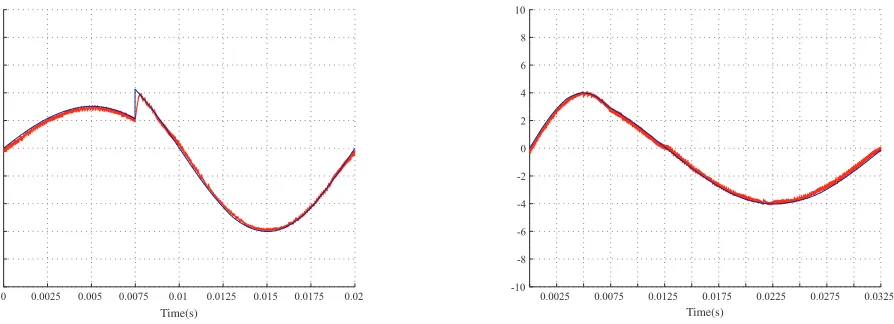
From Fig. 11 to Fig. 14 are presented simulation and experimental results under frequency and amplitude variations. There is observed a very good dynamic responde without any significant overshoot or delay. With these results, the feasibility of the proposed strategy is demonstrated, with no modulators and linear controllers needed, obtaining very good dynamic response with only the prediction of the output current for each valid switching state and the optimization of

0 0.01 0.02 0.03 0.04 0.05 0.06 −10

−5 0 5 10

0 0.01 0.02 0.03 0.04 0.05 0.06 −200

−100 0 100 200 a)

b)

Time(s)

Fig. 5. Simulation results in steady state:𝑖_𝑜 = 6 Apk;𝑓_𝑜 = 50 Hz;𝑓_𝑠 = 40 kHz;𝑣_𝑖= 112 Vpk;

0 0.01 0.02 0.03 0.04 0.05 0.06 −10

−5 0 5 10

0 0.01 0.02 0.03 0.04 0.05 0.06 −200

−100 0 100 200 a)

b)

Time(s)

Fig. 6. Experimental results in steady state:𝑖_𝑜 = 6 Apk;𝑓_𝑜 = 50 Hz;𝑓_𝑠 = 40 kHz;𝑣_𝑖= 112 Vpk;

TABLE III

MEAN AVERAGE ERROR OF𝑖_𝑟𝑒𝑓 VERSUS𝑖_𝑜A UNA𝑓_𝑜= 50 HZ

Sampling (𝑓_𝑠) Amplitude (𝑖_𝑜) Error (𝑒_𝑠𝑖𝑚) Error (𝑒_𝑒𝑥𝑝)

10 kHz 2 Apk 6,994% 8,294%

10 kHz 6 Apk 4,732% 6,640%

20 kHz 2 Apk 4,192% 5,541%

20 kHz 6 Apk 2,869% 4,796%

40 kHz 2 Apk 2,097% 5,181%

40 kHz 6 Apk 1,425% 5,112%

the cost function at every sampling time𝑇_𝑠.

V. CONCLUSION

0.01 0.015 0.02 0.025 0.03 0.035 0.04 0.045 0.05 −10

−5 0 5 10

0.01 0.015 0.02 0.025 0.03 0.035 0.04 0.045 0.05 −200

−100 0 100 200 a)

b)

Time(s)

Fig. 7. Simulation results in transient state:𝑖_𝑜=3-6 Apk;𝑓_𝑜 = 50 Hz;𝑓_𝑠 = 10 kHz;𝑣_𝑖 = 112 Vpk;

0.01 0.02 0.03 0.04 0.05 0.06 0.07 −10

−5 0 5 10

0.01 0.02 0.03 0.04 0.05 0.06 0.07 −200

−100 0 100 200 a)

b)

Time(s)

Fig. 8. Simulation results in transient state:𝑖_𝑜 = 4 Apk;𝑓_𝑜 = 50-25 Hz;𝑓_𝑠 = 20 kHz;𝑣_𝑖 = 112 Vpk;

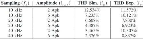
TABLE IV

TOTAL HARMONIC DISTORTION OF THE LOAD CURRENT@𝑓_𝑜= 50 HZ

Sampling (𝑓_𝑠) Amplitude (𝑖_𝑟𝑒𝑓) THD Sim. (𝑖_𝑜) THD Exp. (𝑖_𝑜)

10 kHz 2 Apk 12,534% 11,572%

10 kHz 6 Apk 7,235% 10,121%

20 kHz 2 Apk 6,608% 7,830%

20 kHz 6 Apk 4,387% 6,923%

40 kHz 2 Apk 3,465% 10,307%

40 kHz 6 Apk 2,376% 8,837%

presented strategy provides good tracking of the output current to its reference.

ACKNOWLEDGMENTS

This publication was made possible by the Newton Picarte Project EPSRC: EP/N004043/1: New Configurations of Power Converters for Grid Interconnection Systems / CONICYT DPI20140007 and British Council through the Institutional Skills Development Newton Picarte Project ISCL 2015006.

0.03 0.035 0.04 0.045 0.05 0.055 0.06 0.065 0.07 −10

−5 0 5 10

0.03 0.035 0.04 0.045 0.05 0.055 0.06 0.065 0.07 −200

−100 0 100 200 a)

b)

Time(s)

Fig. 9. Experimental results in transient state:𝑖_𝑜 = 3-6 Apk;𝑓_𝑜 = 50 Hz;𝑓_𝑠 = 10 kHz;𝑣_𝑖= 112 Vpk.

0.03 0.04 0.05 0.06 0.07 0.08 0.09 −10

−5 0 5 10

0.03 0.04 0.05 0.06 0.07 0.08 0.09 −200

−100 0 100 200 a)

b)

Time(s)

Fig. 10. Experimental results in transient state:𝑖_𝑜 = 4 Apk;𝑓_𝑜 = 50-25 Hz;

𝑓𝑠 = 20 kHz;𝑣𝑖 = 112 Vpk;

REFERENCES

[1] E. Yamamoto, T. Kume, H. Hara, T. Uchino, J. Kang, and H. Krug, “Development of matrix converter ans its applications in industry,”35th Annual Conference of the IEEE Industrial Electronics Society IECON 2009, Porto, Portugal, 2009.

[2] M. Venturini, “A new sine wave in sine wave out, conversion technique which eliminates reactive elements,”Powercon 7, 1980, pp. E3/1–E3/15, Mar. 2001.

[3] J. Rodriguez, E. Silva, F. Blaabjerg, P. Wheeler, J. Clare, and J. Pontt, “Matrix converter controlled with the direct transfer function approach: analysis, modelling and simulation,” Taylor and Francis-International Journal of Electronics, vol. 92, no. 2, pp. 63 –85, Feb. 2005. [4] L. Zhang, C. Watthanasarn, and W. Shepherd, “Control of ac-ac matrix

converters for unbalanced and/or distorted supply voltage,”Power Elec-tronics Specialists Conference, 2001. PESC. 2001 IEEE 32nd Annual, vol. 2, pp. 1108 –1113 vol.2, 2001.

[5] E. Yamamoto, H. Hara, T. Uchino, M. Kawaji, T. Kume, J. K. Kang, and H.-P. Krug, “Development of mcs and its applications in industry [industry forum],”Industrial Electronics Magazine, IEEE, vol. 5, no. 1, pp. 4 –12, march 2011.

0 0.0025 0.005 0.0075 0.01 0.0125 0.015 0.0175 0.02 -10

-8 -6 -4 -2 0 2 4 6 8 10

Time(s)

Fig. 11. Simulation results in transient state:𝑖_𝑜 = 3-6 Apk;𝑓_𝑜 = 50 Hz;𝑓_𝑠 = 40 kHz;𝑣_𝑖 = 112 Vpk;

0 0.0025 0.005 0.075 0.01 0.0125 0.015 0.0175 0.02 -10

-8 -6 -4 -2 0 2 4 6 8 10

Time(s)

Fig. 12. Experimental results in transient state:𝑖_𝑜 = 3-6 Apk;𝑓_𝑜 = 50 Hz;

𝑓𝑠= 40 kHz;𝑣𝑖 = 112 Vpk;

with power transistors,”Electric Power Applications, IEE Proceedings B, vol. 134, no. 1, p. 9, Jan. 1987.

[8] L. Huber and D. Borojevic, “Space vector modulated three-phase to three-phase matrix converter with input power factor correction,” Indus-try Applications, IEEE Transactions on, vol. 31, no. 6, pp. 1234 –1246, Nov. 1995.

[9] F. Blaabjerg, D. Casadei, C. Klumpner, and M. Matteini, “Comparison of two current modulation strategies for matrix converters under unbalanced input voltage conditions,”Industrial Electronics, IEEE Transactions on, vol. 49, no. 2, pp. 289 –296, Apr. 2002.

[10] I. Takahashi and T. Noguchi, “A new quick response and high efficency control strategy for an induction motor,”Industrial Electronics, IEEE Transactions on, vol. 22, no. 5, pp. 820 –827, Sep. 1986.

[11] S. Muller, U. Ammann, and S. Rees, “New time-discrete modulation scheme for matrix converters,”Industrial Electronics, IEEE Transactions on, vol. 52, no. 6, pp. 1607 – 1615, Dec. 2005.

[12] M. Rivera, R. Vargas, J. Espinoza, and J. Rodriguez, “Behavior of the predictive dtc based matrix converter under unbalanced ac-supply,” Power Electronics Specialists Conference, 2008. PESC 2008. IEEE, pp. 202 –207, Sep. 2007.

[13] M. Rivera, C. Rojas, J. Rodriguez, P. Wheeler, B. Wu, and J. Espinoza, “Predictive current control with input filter resonance mitigation for a direct matrix converter,”IEEE Trans. Power Electron., vol. 26, no. 10, pp. 2794–2803, Oct. 2011.

[14] S. Kouro, P. Cortes, R. Vargas, U. Ammann, and J. Rodriguez, “Model predictive control-A simple and powerful method to control power

0.0025 0.0075 0.0125 0.0175 0.0225 0.0275 0.0325 -10

-8 -6 -4 -2 0 2 4 6 8 10

Time(s)

Fig. 13. Simulation results in transient state:𝑖_𝑜 = 4 Apk;𝑓_𝑜 = 50-25 Hz;𝑓_𝑠 = 40 kHz;𝑣_𝑖= 112 Vpk;

0.0025 0.0075 0.0125 0.0175 0.0225 0.0275 0.0325 -10

-8 -6 -4 -2 0 2 4 6 8 10

Time(s)

Fig. 14. Experimental results in transient state:𝑖_𝑜 = 4 Apk;𝑓_𝑜 = 50-25 Hz;

𝑓𝑠 = 40 kHz;𝑣𝑖 = 112 Vpk;

converters,”IEEE Trans. Ind. Electron., vol. 56, no. 6, pp. 1826–1838, Jun. 2009.

[15] J. Rodriguez, M. P. Kazmierkowski, J. R. Espinoza, P. Zanchetta, H. Abu-Rub, H. A. Young, and C. A. Rojas, “State of the art of finite control set model predictive control in power electronics,”IEEE Trans. Ind. Informat., vol. 9, no. 2, pp. 1003–1016, May. 2013.

[16] C. Rojas, J. Rodriguez, A. Iqbal, H. Abu-Rub, A. Wilson, and S. Moin Ahmed, “A simple modulation scheme for a regenerative cascaded matrix converter,” inIECON 2011 - 37th Annual Conference on IEEE Industrial Electronics Society, nov. 2011, pp. 4361 –4366. [17] J. Rodriguez and P. Cortes,Predictive Control of Power Converters and

Electrical Drives, 1st ed. Chichester, UK: IEEE Wiley press, Mar. 2012.

[18] V. Yaramasu, M. Rivera, B. Wu, and J. Rodriguez, “Model predictive current control of two-level four-leg inverters - part I: Concept, algorithm and simulation analysis,”IEEE Trans. Power Electron., vol. 28, no. 7, pp. 3459–3468, Jul. 2013.