Recursive right tailed unit root tests for an explosive asset price bubble

Recursive right-tailed unit root tests for an explosive

asset price bubble

David I. Harvey

, Stephen J. Leybourne

and Robert Sollis

_{School of Economics, University of Nottingham}

yy

_{Newcastle University Business School}

October 2013

Abstract

In this paper we compare the local asymptotic and nite sample power of two recently proposed recursive right-tailed Dickey-Fuller-type tests for an explosive rational bubble in asset prices. It is shown that the power of the two tests can dif-fer substantially depending on the location of the explosive regime, and whether such a regime ends in collapse. Since this information is typically unknown to the practitioner, we propose a union of rejections strategy that combines infer-ence from the two individual tests. We nd that, for a given speci cation of the explosive regime, the union of rejections strategy always attains power close to the better of the individual tests considered. An empirical illustration using the Nasdaq composite price index is also provided.

Keywords: Rational bubble; Explosive autoregression; Unit root testing.

JEL Classi cation: C22; C12; G14.

1

Introduction

A substantial body of theoretical and empirical research exists on statistically testing for explosive asset price bubbles. Much of this literature has concentrated on the class of \rational" explosive asset price bubbles where, despite the asset being overvalued, it is still rational for investors to buy additional units because of the returns available relative to the risk-free discount rate. Orthodox nancial theory suggests that the presence of explosive rational asset price bubbles should be relatively easy to uncover

using simple econometric techniques. Consider for example the standard present value model for the fundamental price of a stock P_tf

P_tf =

1

X

i=1

(1 +r) iEt(Dt+i)

whereDtdenotes the dividend andrdenotes the risk-free discount rate. If the

transver-sality condition lim

n!1Et[(1 +r)

n_P

t+n] = 0 holds, then it can be shown via the standard

no arbitrage condition that the current price of the stock Pt will be equal to the

fun-damental price P_tf. However if the transversality condition above does not hold an explosive rational bubble can exist and the price can be decomposed into the funda-mentals component P_tf and a bubble component Bt, i.e.

Pt=Ptf +Bt

where Bt grows with an expected growth rate equal to r. There are in nitely many

models for Bt that satisfy this condition and so a de nitive test for the presence of

a particular type of rational asset price bubble is not feasible. However, it follows straightforwardly from the representation above that if an asset price is not more explosive than the fundamentals component of the price, then a bubble does not exist. In seminal work on this issue, drawing on the fact that an explosive series is also explosive in rst di erences, Diba and Grossman (1988) proposed testing the hypothesis of no explosive rational asset price bubble using standard left-tailed Dickey-Fuller (DF) unit root tests applied to stock price and dividends series in levels and rst di erences, with the absence of an explosive rational bubble inferred from a nding of stationarity in the rst di erences of stock prices.

More direct approaches to identifying explosive rational bubbles have subsequently been proposed, using right-tailed DF tests to detect explosive autoregressive behaviour in stock price series. Hall et al. (1999) initially considered an approach based on Markov-switching autoregressive models, but more recent work in this area has fo-cused on using recursive DF-type tests. Speci cally, Phillips et al. (2011) (PWY) suggest detecting explosive rational bubbles using the supremum of a set of forward recursive DF tests applied to the asset price and the relevant fundamentals series, while Homm and Breitung (2012) (HB) recommend using the supremum of a set of backward recursive (DF-type) Chow tests for a change from unit root to explosive autoregressive behaviour. PWY subsequently advocate using their forward recursive statistics to con-struct a method for time-stamping the start and end dates of the explosive regime; HB suggest an alternative method for dating the origination of explosive behaviour based on their backward recursive approach.

form of collapse (see, for example, Evans, 1991), we include DGP designs that allow for such behaviour. Speci cally, in addition to explosive periods that run up to the end of the sample, we consider non-collapsing explosive periods that return to random walk behaviour at some point prior to the sample's end, and also cases where the post-explosive random walk regime is re-initialized at its pre-post-explosive level, modelling a bubble that terminates with instantaneous collapse.

The results from our asymptotic and nite sample simulations are important for practitioners as they reveal that the relative performance of the tests can di er quite dramatically depending on the location and timing of the explosive regime, and also whether or not the explosive period terminates in collapse. Overall, we nd that the PWY test is better suited to detecting explosive regimes than the HB test when the period of explosiveness occurs early or towards the middle of the sample, while the HB test is better when this regime occurs towards the end of the sample, provided the explosive period does not end in collapse. These results raise the interesting pos-sibility that when the timing of the bubble is unknown, as it would be in practice, a composite test based on a union of rejections strategy applied to the PWY and HB test statistics could yield bene ts to practitioners relative to either of these tests being used individually. This type of strategy, based on rejecting the null hypothesis if any of a number of individual tests indicate rejection, has previously been employed in the literature on testing for a unit root against a stationary alternative, for example when uncertainty exists regarding the presence of a trend in the data, or when uncertainty surrounds the nature of the initial value of the series (see Harvey et al., 2009, 2012). We propose such a strategy involving the PWY and HB tests which is asymptotically correctly sized under the null hypothesis, and compare its power performance with that of the individual tests using local asymptotic and nite sample simulations. We nd that, for a given speci cation of the explosive regime, the union of rejections approach displays power close to the better of the individual PWY and HB tests.

The next section of the paper brie y outlines the original PWY and HB tests. Section 3 presents our model, derives the local asymptotic distributions of the tests, and discusses the results from our asymptotic simulations to assess the power of the original tests when explosive periods of varying timings and durations are present. Section 4 reports the ndings of our nite sample simulations, where a close correspondence to the asymptotic results is seen. Section 5 details the union of rejections strategy proposed and evaluates the asymptotic and nite sample power of this approach relative to that of the individual PWY and HB tests. Section 6 applies the tests to the Nasdaq composite price index, and Section 7 concludes. The following notation is used: `<sub>b c</sub>' denotes the integer part, `_!d' denotes weak convergence, `_!p ' denotes convergence in probability, and _I(:) denotes the indicator function.

2

Recursive right-tailed unit root tests

Consider an observed time series yt, t = 1; :::; T, where our interest focuses on testing

the null that yt follows a unit root AR(1) process throughout the full sample, against

sub-period of the sample. In this context, and in the absence of knowledge concerning the timing of any potential explosive behaviour, PWY propose a test based on the supremum of recursive right-tailed DF tests. Speci cally, the test statistic is given by

PWY = sup

2[ 0;1]

DF

whereDF denotes the standard DF test, that is thet-ratio on ^ in the tted ordinary least squares (OLS) regression

yt = ^ + ^PWYyt 1+ ^"t (1)

calculated over the sub-sample period t = 1; :::;_b T_c, i.e.

DF = _q ^PWY

^2_PWY Pb_t=2Tc(yt 1 y ) 2

where y = (_b T_c 1) 1P_tb₌₂Tcyt 1 and ^2PWY = (b Tc 3) 1

Pb Tc

t=2 ^" 2

t. The PWY

statistic is therefore the supremum of a sequence of forward recursive statistics with minimum sample length _b 0Tc.

HB propose an alternative approach, based on the supremum of recursive Chow tests. Assuming a structure for the alternative hypothesis that speci es yt as a unit

root process up to some change-point _b T_c, and explosive thereafter, they consider structural change tests based on the tted full-sample OLS regression

~

yt= ^HBI(t >b Tc)~yt 1+ ^et (2)

where, in the case where the series is permitted to have a non-zero mean, ~yt = yt y

(i.e. full-sample OLS demeaned). The Chow (DF-type) statistic in this setting is given by the t-ratio on ^_HB, which we denote by C :

C =

^

HB

q

^2_HB PT_{t=b Tc+1}y~2

t 1

where ^2_HB = (T 2) 1PT t=2e^

2

t. HB then propose the test statistic

HB = sup

2[0;1 0]

C

i.e. the supremum of a sequence ofbackward recursive statistics, with minimum poten-tial explosive regime length_b 0Tc. Both the PWY and HB statistics can be adjusted

to account for additional serial correlation in yt via the usual lagged di erence

3

Model and asymptotic results

To evaluate the performance of PWY and HB in detecting explosive, and potentially collapsing, bubble behaviour, we will consider the following model

yt=

8 < :

yt 1+vt t= 2; :::;b 1Tc

(1 + )yt 1+vt t=b 1T + 1c; :::;b 2Tc

yt 1+vt t=b 2T + 2c; :::; T

(3)

with 0, y1 = v1 and yb 2Tc+1 = yb 2Tc + vb 2Tc+1 +y I( > 0). Here, vt is

assumed to follow a martingale di erence sequence with conditional variance 2 _and

sup_tE("4_t)<₁, with v1 =op(T 1=2).

This DGP imposes a unit root on yt up to time b 1Tc, after which yt is explosive

when > 0 until time _b 2Tc. In the third regime, the series reverts to unit root

behaviour, and we consider two speci cations for the initialization of this latter regime: Case 1. y = 0, so that the unit root process is initialized at the last value of the explosive regime; and Case 2. y = y_{b 1}Tc yb 2Tc, where the nal unit root regime

is initialized at the point prior to the explosive period, modelling the case where the explosive bubble collapses and the level of the series reverts to its pre-explosive value, cf. equation (14) in PWY and the subsequent discussion therein. (Note that the y

adjustment plays no role when = 0.) We de ne the null and alternative hypotheses

H0 : = 0 andH1 : >0.

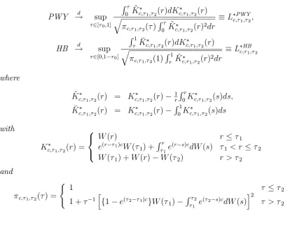
For local alternative hypotheses of the form =c=T, c >0, the following Theorem gives the asymptotic properties of PWY and HB.

Theorem 1 (i) For Case 1,

PWY _!d sup

2[ 0;1]

R

0 K~c; 1; 2(r)dKc; 1; 2(r)

qR

0 K~c; 1; 2(r)2dr

LPWY_{c; 1; 2};

HB _!d sup

2[0;1 0]

R1

Kc; 1; 2(r)dKc; 1; 2(r)

qR1

Kc; 1; 2(r)2dr

LHB_c;

1; 2

where

~

Kc; 1; 2(r) = Kc; 1; 2(r)

1

r

Rr

0Kc; 1; 2(s)ds;

Kc; 1; 2(r) = Kc; 1; 2(r)

R1

0Kc; 1; 2(s)ds

with

Kc; 1; 2(r) =

8 < :

W(r) r 1

e(r 1)c_W(

1) +

Rr

1e

(r s)c_dW(s)

1 < r 2

e( 2 1)c_W(

1) +

R 2

1 e

( 2 s)c_{dW(s) +W(r) W(}

2) r > 2

(ii) For Case 2,

PWY _!d sup

2[ 0;1]

R

0 K~c; 1; 2(r)dKc; 1; 2(r)

q

c; 1; 2( )

R

0 K~c; 1; 2(r)

2_dr

L_c;PWY_{1; 2};

HB _!d sup

2[0;1 0]

R1

K_{c; 1; 2}(r)dK_{c; 1; 2}(r)

q

c; 1; 2(1)

R1

K_{c; 1; 2}(r)2_dr

L_c;HB_{1; 2}

where

~

K_{c; 1; 2}(r) = K_{c; 1; 2}(r) 1_rR₀rK_{c; 1; 2}(s)ds; K_c;

1; 2(r) = Kc; 1; 2(r)

R1

0Kc; 1; 2(s)ds

with

K_{c; 1; 2}(r) =

8 < :

W(r) r 1

e(r 1)c_W(

1) +

Rr

1e

(r s)c_dW(s)

1 < r 2

W( 1) +W(r) W( 2) r > 2

and

c; 1; 2( ) =

(

1 2

1 + 1h

f1 e( 2 1)c

gW( 1)

R 2

1 e

( 2 s)c_dW(s)

i2

> 2

:

Remark 1 The limit distributions ofPWY andHB under the null hypothesisH0 : =

0 are given by LPWY

0; 1; 2 and L

HB

0; 1; 2, respectively, i.e. the limits obtained from Theorem

1(i) with c set to zero. These null limits continue to hold for serially correlated vt,

provided the usual lagged di erence augmentation is applied to the regressions (1) and (2).

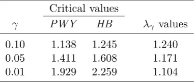
Asymptotic null critical values for 0 = 0:1 (as used in PWY and HB) are

re-ported in Table 1; these were generated by direct simulation of LPWY_{0; 1; 2} and LHB_{0; 1; 2}, approximating the Wiener processes in the limiting functionals usingIID N(0;1) ran-dom variates, with the integrals approximated by normalized sums of 1,000 steps.1

Here and throughout the paper, simulations were conducted using 50,000 Monte Carlo replications.

Figure 1 plots local asymptotic power curves of nominal 0.05-level PWY and HB tests for c _{2 f}0;0:5;1:0; :::;24:0_g, again obtained via direct simulation of the above limits. Figures 1(a) and 1(b) report results where the explosive regime lies in the middle of the sample and Case 1 holds, with ( 1; 2) = (0:45;0:55) in Figure 1(a) and

( 1; 2) = (0:40;0:60) in Figure 1(b), i.e. non-collapsing centrally located explosive

periods of sample proportion duration 0:1 and 0:2, respectively. Figures 1(c) and 1(d)

1_{HB consider the case of no deterministic components iny}

t, and the case of a non-zero mean and

report powers for the same settings as in Figures 1(a) and 1(b), respectively, except now for Case 2, such that the explosive period is collapsing. Figures 1(e) and 1(f) present powers when explosive periods of sample proportion duration 0:1 and 0:2 run up to the end of the sample, i.e. ( 1; 2) = (0:90;1:00) and ( 1; 2) = (0:80;1:00),

respectively (note that in these cases the third regime in (3) is redundant).

Consider rst Figures 1(a) and 1(b), where the explosive period does not collapse. We observe that local asymptotic power increases with the magnitude of the explosive deviation c, and also with the length of the explosive period. The rate of increase is much faster for PWY than for HB, with substantial power advantages o ered by the former test relative to the latter, particularly in the case of the shorter explosive regime.

In Figures 1(c) and 1(d), where the explosive period is now subject to collapse, the power curves for PWY are seen to be largely unchanged from their non-collapsing counterparts. This feature arises since the supremum of the forward recursive statistics involved inPWY tends to occur when the associated sub-sample does not contain the post-explosive period of the data. In contrast, the collapsing explosive regime leads to a dramatic fall in the power levels associated with HB; indeed, power is less than size and approaches zero asc(the locally explosive parameter) increases. This phenomenon is driven by the behaviour of the c; 1; 2(1) term (which is the limit of ^

2

HB= 2) in the

denominator of the limit of HB. This term is a positive random variable for which the mean can be shown to be

E_f c; 1; 2(1)g= 1 + 1(1 e

( 2 1)c₎2₊ e

2( 2 1)c ₁

2c ;

which is an exponentially increasing function of c. Heuristically, as c increases, this term leads to the value of C approaching zero (across all ), and hence HB similarly approaches zero. On an intuitive note, such behaviour is to be expected since, for all

C , ^2_HB is calculated using the full sample of residuals, and is therefore polluted by the impact of the collapse, whose magnitude is an increasing function of . In contrast, for PWY we see that ^2_PWY in DF is calculated using a subset of the data, which is unpolluted by the collapse for any 2; consequently, the PWY supremum is

typically obtained for a DF statistic where 2. Here, c; 1; 2( ) (the limit of

^2_PWY= 2_{) takes a value of unity irrespective of c, and so the behaviour of the error}

variance estimator does not in uence the PWY test statistic in the way that is seen for HB.

polluted by a post-explosive regime, and the supremum of the statistics now tends to occur when the associated sub-sample contains the entirety of the explosive regime.

It is noteworthy that PWY maintains decent levels of power across the di erent explosive settings considered, a property that is not displayed by HB; as such, it is clearly the more reliable of the two procedures. However, it is also apparent that while PWY dominates HB in the majority of cases, when the series under test contains an explosive period that is still operative at the sample end, it is HB that becomes the preferred test. This gives rise to the question of whether a composite procedure can be constructed that capitalizes on the relative advantages of both the individual tests; this is pursued further in section 5 below.

4

Finite sample power comparison

To assess the extent to which these local asymptotic power comparisons are accu-rate predictors of nite sample behaviour, we also consider a number of nite sample simulations. Figures 2 and 3 plot nite sample power curves of nominal 0.05-level PWY and HB tests for T = 300 and T = 600 for _{2 f}0;0:001;0:002; :::;0:080_g and

2 f0;0:001;0:002; :::;0:040_g, respectively (note that = 0:08 and = 0:04 corre-spond to = 1 +c=T with c= 24 when T = 300 and T = 600, respectively, so that the range of values matches those used in the local asymptotic power simulations). Here, vt IID N(0;1) and the settings used for 1 and 2 mirror those of Figure 1,

with both Case 1 (y = 0) and Case 2 (y =y_{b 1}Tc yb 2Tc) again considered. We see

that in each case of Figures 2 and 3, the nite sample powers generally align closely with their local asymptotic counterparts, particularly in the case of the larger sample size T = 600, thus the same comments made above regarding the relative powers of the tests apply equally in nite samples.

In order to assess any possible e ects of non-normality in nite samples, Figure 4 reports nite sample power curves for T = 300 for the same DGPs as in Figure 2, but with vt IID t5. The results are found to be almost identical to those obtained under

normality of the innovations.

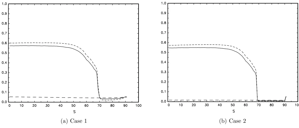
To further explore the e ect that the location of the explosive period, relative to the end of the sample, has on the performance of the test procedures, we undertake the following exercise. We set vt IID N(0;1), T = 300, = 1:05 and ( 1; 2) =

(0:70;0:80) so that an explosive period of length 0:1T occurs relatively late in the sample. We then examine the performance of the tests with the end date of the sample (denoted E) varied from E =_b 1Tc= 210 to E = 300, with the PWY and HB tests

applied to a varying e ective sample size, T , ranging from T = 210 (i.e. observations

simulation for a particular value of E; Figures 5(a) and 5(b) correspond to Case 1 and Case 2, respectively.

Figure 5(a), the case where the explosive regime does not collapse, shows the power of both PWY and HB rising in E as the length of the explosive period increases, up to E = 240, which represents the end of the explosive period. For this range of E, all series contain an explosive regime that runs to the sample's end, and, in line with the results of Figures 1(e) and 1(f),HB is clearly the more powerful test. For larger values of E, where the sample now includes a post-explosive unit root regime of increasing length, the power of PWY stays pretty much constant, while the power of HB starts to decline steadily (becoming lower than that of PWY for, roughly, E > 260). In Figure 5(b), where the explosive regime collapses to pre-explosive levels, the behaviour of the two tests across E up to E = 240 is, of course, identical to that in Figure 5(a). Thereafter, however, while PWY again retains pretty much constant power for larger values ofE, the power of HB falls immediately to zero, and remains there. It is noteworthy that inclusion of as little as one observation of the collapsed regime induces this behaviour.

Figure 6 reports results for a similar simulation exercise, where T = 300 and = 1:05 as before, but now ( 1; 2) = (0:20;0:30), so that the explosive period occurs

relatively early. Here we examine the performance of the procedures with the start date of the sample (denoted S) varied from S= 1 to S =_b 2T + 1c= 91, so that the

PWY and HB tests are again applied to varying e ective sample sizes, ranging from

T = 300 (i.e. observationst= 1; :::;300) toT = 210 (i.e. observationst= 91; :::;300). As S increases, the initial unit root period prior to the explosive regime is decreasing in length, up to the point S = _b 1T + 1c = 61, where no initial unit root period is

present and the series begins explosively. As S increases further, the explosive period now decreases in length, up to the pointS =_b 2T+ 1c= 91, where no explosive period

is now present. As before, Figures 6(a) and 6(b) correspond, respectively, to Case 1 and Case 2.

In both Figures 6(a) and 6(b) we observe that HB only ever has trivial levels of power across S. This arises because there is always a post-explosive unit root regime of long duration (210 observations) present in the sample irrespective of the value ofS. As regards PWY, it has decent, and roughly constant, power for up to about S = 50, after which point the reduced sample size negatively a ects power, particularly for

S > 61 where less observations of the explosive period are included in the sample.

For S 69, the minimum sample length constraint on the set of DF statistics over which the supremum is taken results in all such statistics being calculated over a sub-sample that includes observations from the post-explosive regime; this has the e ect of reducing test power to trivial levels.

5

A union of rejections strategy

In practice we cannot assume knowledge of where in a given sample an explosive regime occurs (should one occur at all); nor can we assume whether or not such a regime is associated with a collapse. In such situations it is therefore unclear as to which ofPWY and HB will have the greater potential to detect explosive behaviour. One strategy would be to simply apply PWY alone since post-explosive unit root regimes do not have the potential to dramatically lower its power, unlikeHB. Such an approach would, of course, mean we sacri ce the power advantage o ered by HB when post-explosive unit root regimes do not cause low power issues (for example, when the explosive period runs to the sample end-point).

We now consider the possibility of harnessing the desirable properties of both tests using a hybrid procedure based onPWY and HB. The approach we adopt here is the following simple union of rejections decision rule:

UR: Reject H0 if PWY > cvPWY orHB > cvHB

wherecvPWY and cvHB denote the asymptotic null critical values of PWY and HB for a signi cance level (see Table 1). Here is a scaling constant calculated such that the asymptotic size associated with UR is equal to the nominal size . The decision rule UR can also be written as

RejectH0 if max PWY;

cvPWY

cvHB HB > cv

PWY ₍₄₎

where, for = 0,

max PWY;cv_cvPWYHB HB

d

!max LPWY_0;

1; 2;

cvPWY

cvHB L

HB

0; 1; 2 (5)

and for = 1 +c=T,c >0,

max PWY;cv_cvPWYHB HB

d

!

8 < :

max LPWY

c; 1; 2;

cvPWY

cvHB LHB_{c; 1; 2} Case 1

max L_c;PWY_{1; 2};cv

PWY

cvHB L

HB

c; 1; 2 Case 2

: (6)

At a given signi cance level , the appropriate value for the constant is obtained by simulating the limit distribution of the right-hand-side of (5), calculating the level critical value for this empirical distribution, say cvU_{, and then computing =}

cvU_=cvPWY_{. These values are given in Table 1 for the conventional signi cance levels.}

to the results in Figure 1. In Figures 5 and 6, the bene ts of UR can again be clearly seen across sample end values, E, and sample start values, S, with UR always closely tracking the power curve of the better performing test across each segment. As such, UR would seem to be a highly e ective means of combining inference from PWY and HB, o ering a size controlled and robust method for the detection of explosive behaviour in a time series.

6

Empirical illustration

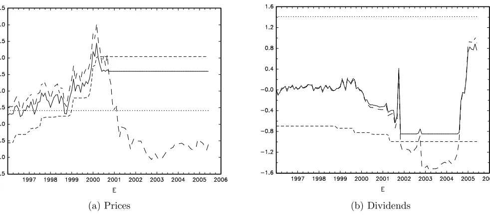
In this section we illustrate the di ering behaviour of the PWY and HB tests, along with the UR strategy, by applying the procedures to monthly data on the Nasdaq composite price index, as used by PWY (and also reconsidered by HB). We employ data over the same period as PWY, i.e. 1973:2-2005:6 (T = 389), using the composite price index adjusted for dividends, and also the composite dividend series derived from the the dividend yields; the data were obtained from Datastream. Logarithms of the real values of the prices and dividends are used, with the nominal data converted using (seasonally adjusted) US consumer price index data obtained from the Federal Reserve Bank of St. Louis. The series are plotted in Figure 7.

In order to assess whether the inference of the tests is sensitive to the end point of the sample (in the manner of the power results reported in Figure 5) we applied the procedures to sample periods from 1973:2 to varying end points from E = 1996:1 to E = 2005:6, this last end date representing the full PWY sample period. When applying thePWY andHB tests, the underlying DF statistics were computed from the OLS regressions (1) and (2) augmented with a number of lagged di erence terms, the number being selected according to the Bayes information criterion, with a maximum of 12, re ecting the monthly nature of the data. Figure 8 reports the results from this application, plotting the PWY and HB statistics across E. In the gures, a straight line is plotted at the level of the asymptotic 0.05-level critical value for PWY (i.e. 1.411, see Table 1), and in order to allow comparison with a common critical value, the reportedHB test statistics are multiplied by the ratio of thePWY andHB asymptotic 0.05-level critical values (i.e. 1.411/1.608 = 0.877). Figure 8 also reports results for the union of rejections strategy UR. In order to again allow comparison with a common critical value, the reported values are max_fPWY;0:877HB_g=1:171, based on (6) with the critical values and value from Table 1.

Indeed, the UR procedure is close to capturing all the rejections of both PWY and HB, with 104 end points out of the 114 considered resulting in a rejection by PWY and/orHB being matched with a rejection byUR. As might be expected, no evidence against the unit root null is found by any of the procedures for the dividend series, suggesting that an explosive period in the price series can be interpreted as a bubble. Visual inspection of the Nasdaq price series plotted in Figure 7 might suggest the presence of explosive bubble behaviour up to the maximum value observed in 2000:3, followed by a collapse thereafter. The pattern of test rejections we obtain are consistent with such a notion, given our earlier simulation results. Speci cally, samples which include a number of post-collapse observations cause HB to fail to detect evidence of a bubble, while these observations have no e ect on PWY. For samples where the putative bubble is still in evidence at the end of the period considered, i.e. pre-2000:3, HB is more likely to detect explosive behaviour than PWY.

From a practitioner's perspective, applying the tests with the bene t of the full sample data spanning 1973:2-2005:6 yields a rejection in favour of bubble behaviour only with PWY. If the tests were applied in 2000:3 (or a number of months either side) then both PWY and HB would have rejected. However, if one were to have implemented the tests prior to 1999 (with the sample therefore ending at such a time), PWY would have failed to nd evidence of a bubble, and a rejection would only have been obtained withHB. This inconsistency of inference associated with PWY and HB is naturally a cause of concern, yet is almost completely eradicated by use of the UR strategy, which would have consistently indicated evidence of a bubble over this period for almost all points in time at which the application was conducted.

7

Conclusion

that in practice it is not known which of PWY or HB would o er the greater ability to detect an explosive bubble, our proposed composite approach o ers a more robust approach to the testing problem, as further evidenced by our empirical illustration, and we envisage it being useful to applied researchers.

While the focus of our analysis has addressed procedures for detecting thepresence of an explosive regime, it is also possible to use the statistics underlying PWY and HB to date the beginning and end of such explosive behaviour. PWY suggest time-stamping the origination and termination of the explosive regime based on the dates for which the DF statistics exceed (diverging) critical values, and a corresponding approach could be developed using theC statistics of HB. An alternative approach to dating the start of an explosive regime is proposed by HB, whereby the argmax of the backward recursive C statistics is employed as a regime-change date estimator, and, once again, a corresponding approach could be devised based on taking the argmax of the forward recursive DF statistics. We leave a proper comparison of such dating schemes, and potential combinations thereof, as an avenue for future research.

References

Diba, B.T. and Grossman, H.I. (1988). Explosive rational bubbles in stock prices? American Economic Review, 78, 520-530.

Evans, G.W. (1991). Pitfalls in testing for explosive bubbles in stock prices. American Economic Review, 81, 922-930.

Hall, S., Psaradakis, Z. and Sola, M. (1999). Detecting periodically collapsing bubbles: a Markov-switching unit root test. Journal of Applied Econometrics, 14, 143-154.

Harvey, D.I., Leybourne, S.J. and Taylor, A.M.R. (2009). Unit root testing in practice: dealing with uncertainty over the trend and initial condition (with commentaries and rejoinder). Econometric Theory, 25, 587-667.

Harvey, D.I., Leybourne, S.J. and Taylor, A.M.R. (2012). Testing for unit roots in the presence of uncertainty over both the trend and initial condition. Journal of Econometrics, 169, 188-195.

Homm, U. and Breitung, J. (2012). Testing for speculative bubbles in stock markets: a comparison of alternative methods. Journal of Financial Econometrics, 10, 198-231.

Phillips, P.C.B. (1987). Towards a uni ed asymptotic theory for autoregression. Biometrika, 74, 535-547.

Appendix: Proof of Theorem 1

(i) By backward substitution in (3) we obtain

yt=

8 > > > < > > > : Pt

i=1vi t= 2; :::;b 1Tc

(1 + )t b 1TcPb 1Tc

i=1 vi+

Pt

i=b 1T+1c(1 + )

t i_v

i t=b 1T + 1c; :::;b 2Tc

(1 + )b 2Tc b 1TcPb 1Tc

i=1 vi

+Pb 2Tc

i=b 1T+1c(1 + )

t i_v i+

Pt

i=b 2T+1cvi

t=_b 2T + 1c; :::; T

(7) and subsequently

T 1=2y_brTc=

8 > > > > > > < > > > > > > :

T 1=2PbrTc

i=1 vi brTc= 2; :::;b 1Tc

(1 + )brTc b 1Tc_T 1=2Pb 1Tc

i=1 vi

+T 1=2PbrTc

i=b 1T+1c(1 + )

brTc i_v

i b

rT_c=_b 1T + 1c; :::;b 2Tc

(1 + )b 2Tc b 1Tc_T 1=2Pb 1Tc

i=1 vi

+Pb 2Tc

i=b 1T+1c(1 + )

brTc i_v

i+T 1=2

PbrTc

i=b 2T+1cvi

brT_c=_b 2T + 1c; :::; T

:

Under =c=T, for 0< a < b <1, (1 + )bbTc baTc_=e(b a)c_{+o(1), and then, following}

Phillips (1987) we nd

1_T 1=2_y

brTc

d

!

8 < :

W(r) r 1

e(r 1)c_W(

1) +

Rr

1e

(r s)c_dW(s)

1 < r 2

e( 2 1)c_W(

1) +

R 2

1 e

( 2 s)c_{dW(s) +W(r) W(}

2) r > 2

= Kc; 1; 2(r):

It is straightforward to show that ^2_PWY = _b T_c 1Pb Tc

t=1 y 2

t +op(1) and ^2HB =

T 1PT

t=1 yt2+op(1). Then, since we can also show that b Tc 1

Pb Tc

t=1 yt2 p

! 2 _for

any , we nd that ^2_{PWY !}p 2 and ^2_{HB !}p 2. The stated limits for PWY and HB then follow from an application of the continuous mapping theorem.

(ii) The limits K_{c; 1; 2}(r) and Kc; 1; 2(r) are identical apart from whenr > 2. In this

case, the third partition of (7) is replaced by

yt= Pb_i=11Tcvi+P_ib₌rT_bc_2T+1cvi; t=b 2T + 1c; :::; T (8)

and then

1

T 1=2y_brTc

d

Using (7) and (8),

yt =

8 > > > > > > > > > > > > < > > > > > > > > > > > > :

vt t = 2; :::;b 1Tc

(1 + )b 1T+1c b 1TcPb 1Tc

i=1 vi

+Pb 1T+1c

i=b 1T+1c(1 + )

b 1T+1c i_v

i

Pb 1Tc

i=1 vi

t =_b 1T + 1c

(1 + )t b 1TcPb 1Tc

i=1 vi+

Pt

i=b 1T+1c(1 + )

t i_v i

(1 + )t 1 b 1TcPb 1Tc

i=1 vi

Pt 1

i=b 1T+1c(1 + )

t 1 i_v i

t =_b 1T + 2c; :::;b 2Tc

Pb 1Tc

i=1 vi+vb 2T+1c (1 + )b

2Tc b 1TcPb 1Tc

i=1 vi

Pb 2Tc

i=b 1T+1c(1 + )

b 2Tc i_v

i

t =_b 2T + 1c

vt t =b 2T + 2c; :::; T

= 8 > > > > > > > > > < > > > > > > > > > :

vt t = 2; :::;b 1Tc

Pb 1Tc

i=1 vi+ (1 + )vb 1T+1c t =b 1T + 1c

vt+

Pt 1

i=b 1T+1c(1 + )

t 1 i_v i

+ (1 + )t b 1Tc 1Pb 1Tc

i=1 vi

t =_b 1T + 2c; :::;b 2Tc

v_{b 2P}T+1c+f1 (1 + )b 2Tc b 1TcgPbi=11Tcvi

b 2Tc

i=b 1T+1c(1 + )

b 2Tc i_v

i

t =_b 2T + 1c

vt t =b 2T + 2c; :::; T

:

Since =c=T we then nd that

yt =

8 > > > > > > > < > > > > > > > :

vt t= 2; :::;b 1Tc

v_{b 1}T+1c+op(1) t=b 1T + 1c

vt+op(1) t=b 1T + 2c; :::;b 2Tc

f1 (1 +c=T)b 2Tc b 1Tc_gPb 1Tc

i=1 vi

Pb 2Tc

i=b 1T+1c(1 +c=T)

b 2Tc i_v

i+op(T 1=2)

t=_b 2T + 1c

vt t=b 2T + 2c; :::; T

:

As regards ^_PWY2 , we can again show that ^2_PWY = _b T_c 1P_tb₌₁Tc y_t2 +op(1). Then

for _b T_{c b} 2Tc, we nd that b Tc 1Pb_t=1Tc y2t = b Tc 1

Pb Tc

t=1 v 2

t +op(1) p

! 2_.

For_b T_c>_b 2Tc, write

b T_c 1Pb_t=1Tc y_t2 =_b T_c 1Pb 2Tc

t=1 y 2

t +b Tc

1Pb Tc

t=b 2Tc+1 y

2

t:

Here

b T_c 1Pb 2Tc

t=1 y 2

t = b Tc

1

b 2Tcb 2Tc 1

Pb 2Tc

t=1 v 2

t +op(1) p

! 2 2:

Also,

b T_c 1Pb_t=T_bc

2Tc+1 y

2

t =b Tc

1 _y2

b 2Tc+1+b Tc

1Pb Tc

t=b 2Tc+2 y

2

t

where

b T_c 1Pb_t=T_bc

2Tc+2 y

2

t = b Tc

1Pb Tc

t=b 2Tc+2v

2

t

= _b T_c 1(_b T_{c b} 2Tc)(b Tc b 2Tc) 1

Pb Tc

t=b 2Tc+2v

2

t p

while

b T_c 1 y_b2

2Tc+1 =

1h

f1 (1 +c=T)b 2Tc b 1Tc

gT 1=2Pb 1Tc

i=1 vi

T 1=2Pb 2Tc

i=b 1T+1c(1 + )

b 2Tc i_v

i

i2

d

! 2 1hf1 e( 2 1)c

gW( 1)

R 2

1 e

( 2 s)c_dW(s)i

2

:

So,

b T_c 1Pb_t=1Tc y_t2 _!d 2+ 2 1h_f1 e( 2 1)c

gW( 1)

R 2

1 e

( 2 s)c_dW(s)

i2

:

Taking the limits together, we see that

^2_{PWY !}d 2

(

1 2

1 + 1h

f1 e( 2 1)c_gW(

1)

R 2

1 e

( 2 s)c_dW(s)

i2

> 2

= 2 c; 1; 2( ):

Finally, for ^2_HB, we can show that ^2_HB = T 1PT t=1 y

2

t +op(1). It follows that its

limit is the same as that of ^2_PWY upon setting = 1, i.e. 2

Table 1. Asymptotic critical values for PWY and HB at the γ significance level, and λγ values for UR

Critical values

γ PWY HB λγ values

0.10 1.138 1.245 1.240

0.05 1.411 1.608 1.171

(a) (τ₁, τ₂) = (0.45,0.55), Case 1 (b) (τ₁, τ₂) = (0.40,0.60), Case 1

(c) (τ₁, τ₂) = (0.45,0.55), Case 2 (d) (τ₁, τ₂) = (0.40,0.60), Case 2

(e) (τ₁, τ₂) = (0.90,1.00) (f) (τ₁, τ₂) = (0.80,1.00)

(a) (τ₁, τ₂) = (0.45,0.55), Case 1 (b) (τ₁, τ₂) = (0.40,0.60), Case 1

(c) (τ₁, τ₂) = (0.45,0.55), Case 2 (d) (τ₁, τ₂) = (0.40,0.60), Case 2

(e) (τ₁, τ₂) = (0.90,1.00) (f) (τ₁, τ₂) = (0.80,1.00)

(a) (τ₁, τ₂) = (0.45,0.55), Case 1 (b) (τ₁, τ₂) = (0.40,0.60), Case 1

(c) (τ₁, τ₂) = (0.45,0.55), Case 2 (d) (τ₁, τ₂) = (0.40,0.60), Case 2

(e) (τ₁, τ₂) = (0.90,1.00) (f) (τ₁, τ₂) = (0.80,1.00)

(a) (τ₁, τ₂) = (0.45,0.55), Case 1 (b) (τ₁, τ₂) = (0.40,0.60), Case 1

(c) (τ₁, τ₂) = (0.45,0.55), Case 2 (d) (τ₁, τ₂) = (0.40,0.60), Case 2

(e) (τ₁, τ₂) = (0.90,1.00) (f) (τ₁, τ₂) = (0.80,1.00)

(a) Case 1 (b) Case 2

Figure 5. Finite sample power across sample end dates, T = 300,δ = 1.05, (τ1, τ2) = (0.70,0.80):

PWY_{: - - - ,} HB_{: – – ,} UR_:

(a) Case 1 (b) Case 2

Figure 6. Finite sample power across sample start dates, T = 300, δ= 1.05, (τ1, τ2) = (0.20,0.30):

(a) Prices (b) Dividends

Figure 7. Logarithms of Nasdaq composite real price index and real dividends, 1973:2–2005:6

(a) Prices (b) Dividends