A double end fault location technique for distribution systems based on fault generated transients

A Double End Fault Location Technique for

Distribution Systems Based on Fault-Generated

Transients

F. M. Aboshady*

_{, Mark Sumner*,}

_{D. W. P. Thomas*}

* Department of Electrical and Electronic Engineering, University of Nottingham, Nottingham, UK

† _{Electrical Power and Machines Engineering Department, Tanta University, Tanta, Egypt}

[email protected]

Abstract— This paper presents a fault location technique for distribution systems. It is a two end impedance based technique that uses the fault generated transients to estimate the fault distance over a broad range of frequencies. Then, curve fitting is applied to find the final estimated fault distance. Firstly, the paper introduces the method for the system represented as a lumped RL model. Then, generalized to consider the distribution line capacitance. The technique accounts for presence of loading taps, heterogeneous feeder sections, single phase, two phase and three phase loads and unbalance in distribution system. Single line to ground, line to line, and three phase faults are considered at different fault resistance values up to 100 Ω. Also, the effect of fault inception angle and resolution of analogue to digital converter is investigated. IEEE 34 nodes system is used to evaluate the proposed method.

Keywords—fault location; fault transients; impedance based techniques.

I. INTRODUCTION

Fast and accurate fault location can improve power system continuity by reducing the time required to locate and repair a permanent fault and therefore reduce the interruption time. It can also help with locating intermittent or high impedance faults, providing information to maintenance teams of the weak points in a system [1]. It is becoming an increasingly important topic as distribution systems become more flexible and complicated for example with the increase of embedded generation.

Several techniques for fault location have been developed based on a variety of methods including apparent impedance, travelling wave, artificial intelligence and disbursed devices based techniques [2]. The impedance based methods mainly use the fundamental frequency components to estimate the fault distance: Furthermore they can be classified to single end and multi terminal techniques based on the availability of measurement points in the system [3-6]. The single end methods are cheap and simple and use iterative approaches to compensate for the unknown fault resistance value and remote end current which in turn affect the method accuracy. On the other hand, multi terminal methods depend on several measurements which

increase both accuracy and cost. Impedance based techniques that use the fault generated high frequencies were reported in [7, 8]. These wideband techniques have the advantage of using a short data window, hence they could be implemented in real time applications with a fast response time. Travelling wave techniques detect the high frequency waves reflected from the fault point and use the arrival time for these waves to the measurement point(s) to estimate the fault distance [9]. Despite of being fast and accurate, they require very high sampling rates in range of MHz or even GHz. Also, for application with distribution systems, the waves will suffer from more reflections and attenuation due to presence of loading taps and lateral connections. Therefore, the implementation of travelling wave based techniques in distribution systems is complex and cost intensive. Artificial intelligence based techniques employ a heuristic way of using the data collected from the system. Using artificial neural networks is an example for such techniques [10]. These methods require extensive training (and retraining if the system topology changes) to accommodate for all possible fault scenarios. Techniques that can benefit from devices installed along the system such as smart meters or fault indicators have been reported [11, 12]. Usually these methods define the closest bus to the fault point instead of the actual fault position. In [11], a method based on matching the recorded voltage sag and the calculated voltage sag simulated at all system nodes was presented: the system node with the highest match is considered to be the faulty or closest node to the fault point. The benefit behind the method is the ability to locate sub-cycle faults. However, it assumed the availability of measurements at all system nodes and will fail if this is not available.

generated from the fault to estimate the fault distance. However, in [7], the algorithm is based on the presence of a re-closer circuit breaker at the beginning of each section in the feeder which is impractical. Only solid faults were examined using this algorithm, hence the accuracy against fault resistance is not guaranteed. In [8], the algorithm assumed the availability of measurements at both ends of every section, and a sampling frequency of 1 MHz was necessary which increases the cost of implementation. When the algorithm was applied to a system with loading taps between the two measurement points, the accuracy was significantly decreased and a percentage error of 25% in the estimated distance was obtained.

The proposed technique only requires a short data window - less than one cycle during and before the fault occurrence - and a sampling frequency of 20 kHz to estimate the fault distance. The method is suitable for real time implementation on a simple microcontroller. Also, it is able to locate sub-cycle faults, helping to reduce the number of unexpected outages. The proposed technique considers the presence of loading taps, non-homogeneous feeder sections, system unbalance, different fault types, different fault resistance values, various fault inception angles and influences from the data acquisition equipment. Also, the derivation considers a distribution system without line capacitance and then is generalized to include the capacitance of the distribution lines.

II. METHODOLOGY

The fault location technique presented in this paper depends on the fault transients generated when a fault occurs. The technique is firstly derived ignoring the line capacitance, then the procedure is generalized to consider the line capacitance. The proposed method is carried out based on phase analysis rather than sequence components analysis to consider the unbalance that might exist in the distribution systems.

A. RL Lumped Parameters System

Assuming a fault at point f between any two nodes S and R, the fault is modelled as a source for a transient at the fault point as shown in Fig. 1. The voltage at point f is obtained by (1) and (2).

Zf

Vfault

xZ (1-x)Z

S R

f

VS, IS VR, IR

Fig. 1. Single line diagram for system with a fault at point f

S S

f V xZI

V   (1)

R R

f V xZI

V  (1 ) (2)

where x is the per unit fault distance measured from node S;

VS and IS are vectors of three phase voltages and currents at

node S; VR and IR are vectors of three phase voltages and

currents at node R; Zf is the fault impedance; Z is the total

section series impedance including both self and mutual impedances.

The voltage and current vectors at nodes S and R, are obtained by wideband measurements at substation downstream and wideband measurements at the feeder end node upstream respectively [14]. By equating (1) and (2), the following equation as a function of the per unit fault distance x is obtained:

R R S R

S I V V ZI

I

xZ(  )   (3)

Equation (3) is used to calculate the three values for x, these values correspond to the three phases. By applying (3) at different frequencies generated from the fault, there will be a series of values for x for each phase. Curve fitting is used to find the most appropriate value of x for each phase. Curve fitting is applied on results within the frequency range 500 Hz to 2000 Hz. The values that correspond to the faulty phases are considered. Also, for multi-phase faults, the average value for the values of x is used as the fault distance, e.g. for a fault between phases A and B, the final fault distance is the average of the two values for x for phases A and B.

B. System with Capacitance

In this part the technique considering the line capacitance is derived. The general configuration is shown in Fig. 2. The same procedure is applied but includes the line capacitance. Here, the line is modelled using the general ABCD parameters. Considering a π model for the system, the values for A1, B1, A2, and B2 as a function of x are given

by (4)

Z x

BI x ZY

A

xZ

BI x ZY

A

) 1 (.5(1 ) 0

5 . 0

2

2 2

1 2 1



 

 

  

(4)

where I is the identity matrix and Y is the total section shunt admittance.

A1 B1

C1 D1

A2 B2

C2 D2

Fault impedance

Vfault

R S

VS, IS VR, IR

f

x 1-x

Also, the voltage at the fault point f is given by (5) and (6)

S S

f AV BI

V  ₁  ₁ (5)

R R

f AV B I

V  ₂  ₂ (6)

By equating (5) and (6) and substituting for the line parameters, a second order equation to find x is obtained.

AA x2 _{+ BB x + CC = 0 (7)}

where,

R R R

S

R S

R

R S

ZI ZYV V

V CC

ZYV I

I Z BB

V V ZY AA

 

 

  

 

5 . 0

) (

) (

5 . 0

(8)

By solving (7), the value of x is calculated and the same procedure of curve fitting to find the final fault distance is followed.

As clear from the previous analysis, the fault distance estimation is independent of the fault resistance and the same equation is applicable for different fault types which allows the method to be simply implemented.

III. CASE STUDY

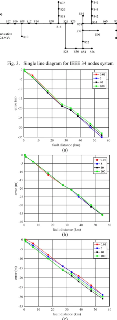
The IEEE 34 nodes system is used to evaluate the performance of the proposed method [15]. The test considers the longest feeder that extends from substation at node 800 to node 848 and the effect of laterals has not been covered in this study. The total length of this feeder is about 58 km. This feeder is characterized by non-homogeneous sections and also the presence of single phase, two phase, and three phase (balanced and unbalanced) loads along the feeder. The simulation is carried out using Matlab/Simulink software with all loads treated as a constant impedance. Three phase voltage and current measurements at nodes 800 and 848 are used by the fault locator. A data window of 30 ms, composed of pre-fault and during-fault segments is enough for the proposed method to estimate the fault distance. A sampling frequency of 20 kHz is used for capturing the signals. Single line to ground, line to line and three phase faults are examined. The effects of fault resistance, fault inception angle and the use of a 16 bit analogue to digital converter resolution on the accuracy of the fault location are studied.

A. Results for RL Lumped Parameters System

1)Effect of fault resistance

Different fault types are simulated along the feeder at fault resistance values of 0.01, 5, 40 and 100 Ω. The fault cases are carried out at fault inception angle of 30º. Fig. 4 presents the error in meters as calculated by (9) for different types of fault.

error = estimated distance — actual distance (9) For different fault resistance values, the error in estimated distance has a very close behavior. This reflects the independency of the proposed method on the fault resistance.

800

806 808 812 814

810

802 850

818 824 826 816

820 822

828 830 854 856 852 832

890

838 862

840 836 860 834

842 844 846

848

864

858

Substation 24.9 kV

Fig. 3. Single line diagram for IEEE 34 nodes system

(a)

(b)

(c)

Fig. 4. Error in estimated distance at different fault resistance values, RL model, for (a) single line to ground fault, (b) lint to line fault and (c) three

phase fault

2) Effect of fault inception angle

Fig. 5. Error in estimated distance for single line to ground fault at different fault inception angles, RL model

It can be seen from Fig.5 that a good estimate of fault location in this system can be achieved even when the phase voltage at the time of the fault is low (ie inception angle of 0° or 180°).

From the previous results, it becomes clear that the proposed method is robust against fault distance, fault type, fault resistance value and the fault inception angle. The maximum absolute error obtained is about 35 m for a 58 km long feeder.

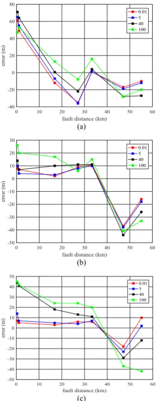
B. Results for System with Capacitance

For these results the model of the line used in the simulation has been modified to incorporate capacitance using the π model, and the fault location method has been modified by using the general ABCD parameters for lines.

For a phase A to ground fault in the section between nodes 854 and 852, Fig. 6 illustrates the captured voltage and current at both measurement points for phase A. The negative time represents the pre-fault period. The oscillations that appear in the voltage signals are due to the effect of the system capacitance.

1)Effect of fault resistance

The three fault types investigated in this paper are carried out at seven points along the feeder at different fault values. All cases consider a fault inception angle of 30º.

Fig. 6. Measured voltage and current for phase A to ground fault

(a)

(b)

(c)

Fig. 7. Error in estimated distance at different fault resistance values, π model, for (a) single line to ground fault, (b) lint to line fault and (c) three

phase fault

2) Effect of fault inception angle

Fig. 8 illustrates the results for three phase faults with a fault resistance value of 5 Ω simulated at five different fault inception angles.

From Fig. 7 and Fig. 8, although the accuracy of the method decreased compared to RL model, the method still works with a high accuracy that does not exceed 80 m.

3) Effect of 16bit ADC resolution

Fig. 8. Error in estimated distance for three phase fault at different fault inception angles, π model

Fig. 9. Error in estimated distance when applying analogue to digital convereter, π model

From all the previous results, the maximum absolute error obtained by the proposed method is less than 100 m for a total feeder length of about 58 km.

IV. CONCLUSION

A fault location technique based on the generated fault transients and using two end measurements has been presented. The technique considered several factors that affect accuracy of the fault location e.g. fault type, fault resistance, fault inception angle and resolution of the data acquisition equipment as well as some characteristics of the distribution system. The technique has the advantage of being fast and accurately pinpointing the fault location which suggests it can be used for real time applications and locating sub-cycle faults. Also, the proposed technique is independent of the fault resistance and the same equation is applicable to different fault types. Under all test conditions provided in this paper, the absolute error obtained was always less than 100 m for a total feeder length of about 58 km. On-going work is investigating how the algorithm can compensate for the presence lateral connections and branches in the distribution system.

ACKNOWLEDGMENT

This work was supported by the Egyptian Government-ministry of higher education (cultural affairs and missions sector) and the British Council through Newton-Mosharafa fund.

REFERENCES

[1] M. M. Saha, J. Izykowski, and E. Rosolowski, Fault location on power networks: Springer, 2010.

[2] M. Abad, M. García-Gracia, N. E. Halabi, and D. L. Andía, "Network impulse response based-on fault location method for fault location in power distribution systems," IET Generation, Transmission & Distribution, vol. 10, pp. 3962-3970, 2016. [3] R. Krishnathevar and E. E. Ngu, "Generalized Impedance-Based

Fault Location for Distribution Systems," IEEE Transactions on Power Delivery, vol. 27, pp. 449-451, 2012.

[4] F. M. Abo-Shady, M. A. Alaam, and A. M. Azmy, "Impedance-based fault location technique for distribution systems in presence of distributed generation," in 2013 IEEE International Conference on Smart Energy Grid Engineering (SEGE), 2013, pp. 1-6.

[5] J. Ramirez-Ramirez, J. Mora-Florez, and C. Grajales-Espinal, "Fault location method based on two end measurements at the power distribution system," in Circuits & Systems (LASCAS), 2015 IEEE 6th Latin American Symposium on, 2015, pp. 1-4.

[6] J. J. Mora-Florez, R. A. Herrera-Orozco, and A. F. Bedoya-Cadena, "Fault location considering load uncertainty and distributed generation in power distribution systems," IET Generation, Transmission & Distribution, vol. 9, pp. 287-295, 2015.

[7] K. Jia, Z. Ren, T. Bi, and B. Liu, "A fault location method based on reclosing in distribution systems," in 2015 5th _{International}

Conference on Electric Utility Deregulation and Restructuring and Power Technologies (DRPT), 2015, pp. 1016-1019.

[8] K. Jia, D. W. P. Thomas, and M. Sumner, "A New double-ended fault-location scheme for utilization in integrated power systems," IEEE Transactions on Power Delivery, vol. 28, pp. 594-603, 2013. [9] A. Dwivedi and X. Yu, "Fault location in radial distribution lines

using travelling waves and network theory," in 2011 IEEE International Symposium on Industrial Electronics, 2011, pp. 1051-1056.

[10] C. Apisit, C. Positharn, and A. Ngaopitakkul, "Discrete wavelet transform and probabilistic neural network algorithm for fault location in underground cable," in 2012 International conference on Fuzzy Theory and Its Applications (iFUZZY2012), 2012, pp. 154-157.

[11] P. C. Chen, V. Malbasa, and M. Kezunovic, "Locating sub-cycle faults in distribution network applying half-cycle DFT method," in T&D Conference and Exposition, 2014 IEEE PES, 2014, pp. 1-5. [12] F. Trindade, W. Freitas, and J. C. d. M. Vieira, "Fault location in

distribution systems based on smart feeder meters," in PES General Meeting | Conference & Exposition, 2014 IEEE, 2014, pp. 251-260. [13] M. Kezunovic, "Smart Fault Location for Smart Grids," IEEE

Transactions on Smart Grid, vol. 2, pp. 11-22, 2011.

[14] W. H. Kersting, Distribution system modeling and analysis, 2 ed.: Taylor & Francis Group, Boca Raton, 2007.

[15] IEEE PES Distribution System Analysis Subcommittee, 34-bus feeder[Online].Available: