An adaptive variable order quadrature strategy

Strategy

Paul Houston and Thomas P. Wihler

AbstractWe propose a new adaptive numerical quadrature procedure which in-cludes both local subdivision of the integration domain, as well as local variation of the number of quadrature points employed on each subinterval. In this way we aim to account for local smoothness properties of the integrand as effectively as possible, and thereby achieve highly accurate results in a very efficient manner. Indeed, this idea originates from so-calledhp-version finite element methods which are known to deliver high-order convergence rates, even for nonsmooth functions.

1 Introduction

Numerical integration methods have witnessed a tremendous development over the last few decades; see, e.g., [2, 3, 14]. In particular, adaptive quadrature rules have nowadays become an integral part of many scientific computing codes. Here, one of the first yet very successful approaches is the application of adaptive Simpson integration or the more accurate Gauss-Kronrod procedures (see, e.g., [7]). The key points in the design of these methods are, first of all, to keep the number of function evaluations low, and, secondly, to divide the domain of integration in such a way that the features of the integrand function are appropriately and effectively accounted for. The aim of the current article is to propose a complementary adaptive quadra-ture approach that is quite different from previous numerical integration schemes. In fact, our work is based on exploiting ideas fromhp-type adaptive finite element

Paul Houston

School of Mathematical Sciences, University of Nottingham, University Park, Nottingham, NG7 2RD, UK, e-mail: Paul.Houston@nottingham.ac.uk

Thomas P. Wihler

Mathematisches Institut, Universit¨at Bern, Sidlerstrasse 5, CH-3012 Bern, Switzerland, e-mail: wihler@math.unibe.ch. TW acknowledges the financial support by the Swiss National Science Foundation (SNF)

methods (FEM); cf. [4, 6, 11, 12, 20]. These schemes accommodate and combine both traditional low-order adaptive FEM and high-order (so-called spectral) meth-ods within a single unified framework. Specifically, their goal is to generate discrete approximation spaces which allow for both adaptively refined subdomains, as well as locally varying approximation orders. In this way, thehp-FEM methodology is able to resolve features of an underlying unknown analytical solution in a highly ef-ficient manner. In fact, this approach has proved to be enormously successful in the context of numerically approximating solutions of differential equations, and has been shown to exhibit high-order algebraic or exponential convergence rates even in the presence of local singularities; cf. [8, 16, 18].

With this in mind, we adopt thehp-adaptive FEM strategy for the purpose of introducing a variable order adaptive quadrature framework. More precisely, we propose a procedure whereby the integration domain will be subdivided adaptively in combination with a local tuning of the number of quadrature points employed on each subinterval. To drive this refinement process, we employ a smoothness es-timation technique from [6, 21] (see also [11] for a related strategy), which was originally introduced in the context ofhp-adaptive FEMs. Specifically, the smooth-ness test makes it possible to gain local information concerning the regularity of the integrand function, and thereby, to suitably subdivide the integration domain and se-lect an appropriate number of quadrature points for each subinterval. By means of a series of numerical experiments we demonstrate that the proposed adaptive quadra-ture strategy is capable of generating highly accurate approximations at a very low computational cost. The main ideas on this new approach together with a view on practical aspects will be discussed in the subsequent section.

2 An

hp

-Type Quadrature Approach

Typical quadrature rules for the approximation of an integralI:=R1

−1f(x)dxof a continuous function f: [−1,1]→_R, take the formI≈Qbp(f):=∑p_k=1wp,kf(bxp,k), where p≥1 is a (typically prescribed) integer number, and{_bxp,k}_kp₌₁⊂[−1,1] and{wp,k}_kp₌₁⊂(0,2]are appropriate quadrature points and weights, respectively. When dealing with a variable number pof quadrature points and weights, we can consider one-parameter families of quadrature rules (such as, for example, Gauss-type quadrature methods); here, for each p∈N, with p≥pmin, where pmin is a minimal number of points, there are (possibly non-hierarchical) families of quadra-ture points_bxxxp={bxp,k}

p

k=1, and weightswwwp={wp,k}_kp=1.

On an arbitrary bounded interval[a,b],a<b, a corresponding integration for-mula can be obtained, for instance, by means of a simple affine scaling φ[a,b]:

[−1,1]→[a,b],x_b7→x=φ[a,b](bx) = 1 2hbx+

1

2(a+b),withh=b−a>0. Indeed, in this caseRb

a f(x)dx≈Q[a,b],p(f):=h/2∑_kp₌₁wp,k(f◦φ[a,b])(xbp,k),wheref:[a,b]→

corresponding quadrature point familiesxxxpare obtained in a straightforward way by lettingxxxp=φ[a,b](bxxxp)(noting thatφ[a,b]is extended componentwise to vectors).

Furthermore, the above construction allows us to define composite quadrature rules, whereby the integral of f is approximated on a collection ofn≥1 disjoint (open) subintervals{Ki}n_i=1of[a,b]with[a,b] =

Sn

i=1Ki, i.e.,I≈∑ni=1QKi,p(f|Ki).

2.1 The Basic Idea:

hp

-Adaptivity

Adaptive quadrature rules usually generate a sequence of repeatedly bisected and possibly non-uniform subintervals{Ki}ni=1,n≥1, of the integration domain [a,b] (i.e., each subintervalKimay have a different lengthhi), with a prescribed and uni-form numberpof quadrature points on each subinterval. With the aim of providing highly accurate approximations with as little computational effort as possible, the novelty of the approach presented in this article is to design an adaptive quadrature procedure, which, in addition to subdividing the original interval[a,b]into appro-priate subintervals, is able to adjust the number of quadrature pointspiindividually within each subintervalKiin an effective way. We note that this idea originates from approximation theory [5, 15] (see also [8]), and has been applied with huge success in the context of FEMs for the numerical approximation of differential equations. Indeed, under certain conditions, the judicious combination of subinterval refine-ments (h-refinement) and selection of local approximation orders (p-refinement), which results in the class of so-calledhp-FEMs, is able to achieve high-order alge-braic or exponential rates of convergence, even for solutions with local singularities; see, e.g. [18]. In an effort to automate the combinedh- and p-refinement process, a number of hp-adaptive FEM approaches have been proposed in the literature; see, e.g, [13] and the references cited therein. In the current article, we pursue the smoothness estimation approach developed in [6, 21] (cf. also [11]), and translate the idea into the context of adaptive variable order numerical quadrature.

Given a subintervalKiwithpiquadrature points, we are given a current approxi-mationQKi,pi(f|Ki)of the subintegral

R

Ki f(x)dx≈QKi,pi(f|Ki).Then, with the aim

of improving the approximate value QKi,pi(f|Ki), in the sense of an hp-adaptive

FEM methodology in one-dimension, we propose two possible refinements ofKi:

(i) h-refinement: The subintervalKi of length hi is bisected into two subinter-valsK_i1andK_i2of equal sizehi/2, and the number p_i of quadrature points is

either inherited to both subintervals or, in order to allow for derefinement with respect to the number of local quadrature points, reduced to pi−1 points. In the latter case, we obtain the potentially improved approximation:

Qh_K

i(f) =QK_i1,max(1,pi−1)(f) +QKi2,max(1,pi−1)(f). (1)

Qp_K

i(f) =QKi,pi+1(f). (2)

In case thatpi=pmax, wherepmaxis a prescribed maximal number of quadra-ture points on each subinterval, we define

Qp_K

i(f) =QKi1,pi(f) +QKi2,pi(f), (3)

whereK_i1andK_i2result from subdividingKias in (i).

In order to determine which of the above refinements is more appropriate for a given subintervalKi, we apply a smoothness estimation idea outlined below. Once a deci-sion betweenh- and p-refinement forKihas been made, the procedure is repeated iteratively for any subintervalsKifor whichQKi,pi(f|Ki)and its refined value

(result-ing from the chosen refinement) differ by at least a prescribed tolerancetol>0.

2.2 Smoothness Estimation

The basic idea presented in the articles [6, 11, 21] is to estimate the regularity of a function to be approximated locally. Then, following along the lines of the hp -approximation approach, if the function is found to be smooth, according to the underlying regularity estimation test, then ap-refinement is performed, otherwise an h-refinement is employed. In [6], the following smoothness indicator, for a (weakly) differentiable function f on an intervalKj, has been introduced (cf. [6, Eq. (3)]):

FKj[f]:=

   

  

kfk_L∞_(K

j)

h−_j1/2kfk_L2_(K

j)+

1 √

2h

1/2

j kf0kL2_(K

j)

if f|Kj 6≡0,

1 if f|Kj ≡0.

(F)

The motivation behind this definition is the well-known continuous Sobolev em-beddingW1,2(Kj),→L∞(Kj), which implies thatFKj[f]≤1 in (F); see [6,

Proposi-tion 1]. We classify fas being smooth onKjifFKj[f]≥τ, for a prescribed

smooth-ness testing parameter 0<τ<1, and nonsmooth otherwise.

To begin, we first consider the special case whenf is a polynomial of degreepj≥ 1. Then, the derivative f(pj−1) _{of order p}

j−1 of f is a linear polynomial, and the evaluation of the smoothness indicatorFKj

h

f(pj−1)i_{from (F) is simple to obtain.}

In fact, let us write f|Kj in terms of a (finite) Legendre series, that is,

f|Kj =

pj

∑

al(bLl◦φK−1j ), (4)

for coefficients a0, . . . ,apj ∈R. Here, bLl, l ≥0, are the Legendre polynomials

of[−1,1]toKj. For f as in (4) it can be shown that

FKj

h

f(pj−1)i₌ 1+ξpj

q 1+1₃ξ_p2

j+

√

2ξpj

, (5)

whereξpj = (2pj−1)

ap j/ap j−1

(provided thatapj−16=0); see [6, Proposition 3].

In particular, this implies that, cf. [6,§2.2],

1 2 ≈

√

3

√

6+1 ≤FKj h

f(pj−1)i_{≤1. (6)}

In the context of the numerical integration rule, the above methodology can be adopted as follows: suppose we are given pj ≥2 quadrature points and weights,

{_bxpj,k}

pj

k=1and{wpj,k}

pj

k=1, respectively. Then,

Z

Kj

f(x)dx≈QKj,pj(f|Kj) =

hj 2

pj

∑

w_pj,k(f◦φKj)(xbpj,k). (7)

We denote the uniquely defined interpolating polynomial off of degreepj−1 at the

given quadrature points byΠKj,pj−1f=∑

pj−1

l=0 bl(Lbl◦φK−1j ).Due to orthogonality of

the Legendre polynomials, we note that

bl= 2l+1

hj

Z

Kj

ΠKj,pj−1f(x)(Lbl◦φK−1j )(x)dx, l=0, . . . ,pj−1.

We further assume that the quadrature rule under consideration is exact for all poly-nomials of degree up to 2pj−2. Thereby,

bl= 2l+1

2 pj

∑

wpj,k(ΠKj,pj−1f)◦φKj(xbpj,k)Lbl(xbpj,k)

=2l+1

2 pj

∑

wpj,k(f◦φKj)(bxpj,k)Lbl(bxpj,k).

Consequently, we infer that

ξKj,pj−1:= (2pj−3)

bpj−1

bpj−2

= (2pj−1)

∑_kp₌j₁wpj,k(f◦φKj)(bxpj,k)bLpj−1(xbpj,k)

∑_kp=j1wpj,k(f◦φKj)(bxpj,k)bLpj−2(xbpj,k)

,

(8)

and thus, in view of (5), we use the quantity

FKj,pj(f):=

1+ξKj,pj−1

q 1+1₃ξ_K2

j,pj−1+

√

2ξKj,pj−1

∈ √

3

√

6+1,1 !

cf. (6), to estimate the smoothness of f|Kj. We note that the computation ofξKj,pj−1

does not require any additional function evaluations of f since the values (f◦

φKj)(bxpj,k),k=1, . . . ,pj, have already been determined in the application of (7).

2.3 Adaptive Variable Order Procedure

Based on the above derivations, we propose anhp-type adaptive quadrature method. To this end, we start by choosing a tolerance tol>0, a smoothness parame-terτ∈

√

3_/(√6+1),1, and a maximal numberpmax≥2 of possible quadrature points on each subinterval. Furthermore, we define the interval K1= [a,b], and a small numberp1, 2≤p1≤pmax, of quadrature points onK1. Moreover, we initialise the set of subintervals subs, the order vector pcontaining the number of quadrature points on each subinterval, and the unknown value Q of the integral as follows: subs={K1},p={p1},Q=0. Then, the basic adaptive procedure is given by:

1: whilesubs6=/0do

2: [Q1,subs,p] =hprefine(f,subs,p,pmax,τ); 3: Q=Q+Q1;

4: end while 5: OutputQ.

Here, hprefine is a function, whose purpose is to identify those subintervals insubs, which need to be refined further for a sufficiently accurate approxima-tion of the unknown integral. In addiapproxima-tion, it outputs a set of subintervals (again denoted bysubs), as well as an associated order vector (again denoted byp) which result from applying the most appropriate refinement, i.e., eitherh- orp-refinement as outlined in (i) and (ii) in Section 2.1 above, for each subinterval. Furthermore, hprefinereturns the sumQ1 of all quadrature values corresponding to subintervals in the input setsubsfor which no further refinement is deemed necessary. The es-sential steps are summarised in Algorithm 1; here,pmindenotes the minimal number of quadrature points to be employed on any given subinterval.

2.4 Practical Aspects

In this section we discuss the practical issues involved in the implementation of the procedure described in Section 2.3 within a given computing environment.

2.4.1 Gauss-Quadrature Rules

Algorithm 1Function[Q,subsnew,pnew] =hprefine(f,subs,p,pmin,pmax,τ) 1: Definesubsnew=subs, andpnew=p. SetQ=0.

2: foreach subintervalKj∈subsdo

3: Evaluate the smoothness indicatorFKj,pj(f)from (9). 4: ifFKj,pj(f)<τthen

5: Applyh-refinement toKj, i.e., bisectKjinto two subintervals of equal size and reduce the number of quadrature points to max(pj−1,pmin)on both of them;

6: Compute an improved approximation, denoted byQeKj, ofQKj,pj(f|Kj)using (1) onKj.

7: else ifFKj,pj(f)≥τandpj+1≤pmaxthen

8: Apply p-refinement toKj, i.e., increase the number of quadrature points topj+1 onKj;

9: Compute an improved approximation, denoted byQeKj, ofQKj,pj(f|Kj)using (2) onKj. 10: else ifFKj,pj(f)≥τandpj+1>pmaxthen

11: BisectKj into two subintervals of equal size and retain the number of quadrature pointspjon both of them;

12: Compute an improved approximation, denoted byQeKj, ofQKj,pj(f|Kj)using (3) onKj.

13: end if

14: if|QeKj−QKj,pj(f|Kj)|is sufficiently smallthen

15: UpdateQ=Q+QeKj;

16: EliminateKjfromsubsnewand the corresponding entrypjfrompnew. 17: else

18: ReplaceKjand pj insubsnewandpnew, respectively, by the corresponding h- or p-refined subintervals as determined above.

19: end if

20: end for

of) Gauss-type quadrature schemes. We emphasise, however, that more traditional schemes, including, for example, (fixed-order) Gauss-Kronrod or Clenshaw-Curtis rules, which are naturally hierarchical, may be employed as well (where the de-gree of exactness 2p−2 is desirable with regards to an accurate computation of the smoothness estimation, cf. Section 2.2). Incidentally, our numerical results in-dicate that, although non-hierarchical rules do not support the repeated use of all previously computed function evaluations, their potentially superior degree of ac-curacy, compared to their embedded counterparts, can be exploited very favourably within the hp–setting. Indeed, it is a well-known feature ofhp-methods that they are particularly effective on a variable high-order level, cf., e.g., [17, 18].

weights of the correspondingp-point Gauss-Legendre quadrature rule, respectively (and complementing the remaining entries in all but the last column by zeros):

X XX=



        b

x2,1xb3,1· · · bxpmax,1

b x2,2 ...

b

x3,3 ...

0

xpmax,pmax



       

, WWW = 

       

w2,1w3,1· · · wpmax,1

w2,2 ...

w3,3 ...

0

wpmax,pmax



       

. (10)

We note that, for other quadrature rules, the number of rows in the above matrices may be different.

2.4.2 Vectorised Quadrature

Following the ideas of [19] we use a vectorised quadrature implementation. This means that, instead of computing the integrals on the subintervals subs in Al-gorithm 1 one at a time, they are all computed at once. This can be accom-plished by using fast vector- and matrix-operations, and by carrying out all nec-essary function evaluations in a single operation by computing the function to be integrated for a vector of input values. Specifically, we write the composite rule I≈∑Ki∈subsQKi,pi(f|Ki) =∑Ki∈subshi/2∑

pi

k=1wpi,k(f◦φKi)(bxpi,k)as a dot product

of a weight vector www and a function vector f(xxx); here, the former vector con-tains all (scaled) weights{1

2hiwpi,k}i,k, and the latter vector represents the

evalu-ation of the integrand function f on the vectorxxxof all corresponding quadrature points{φKi(bxpi,k)}i,k appearing in the sum above. Evidently, these vectors can be

built efficiently by extracting (and affinely mapping and scaling) the corresponding rows from the matricesXXX andWWW in (10). We emphasise that applying vectorised quadrature crucially improves the performance of the overall adaptive procedure (provided that such a technology is available in a given computing environment).

2.4.3 Smoothness Estimators

L L L1=



       

L1(bx2,1)L2(bx3,1)· · · Lpmax−1(xbpmax,1)

L1(bx2,2) .. .

L2(bx3,3)

.. .

0

Lpmax−1(bxpmax,pmax) 

       

, (11)

and

L L L2=



       

L0(bx2,1)L1(bx3,1)· · · Lpmax−2(xbpmax,1)

L0(bx2,2) .. .

L1(_bx3,3) ...

0

Lpmax−2(_bxpmax,pmax) 

       

. (12)

Then, the sums in (8) are vectorised similarly as described above. In particular, the computation of the smoothness estimators can be undertaken with an almost negligible computational cost.

2.4.4 Stopping Criterion

In order to implement the stopping-type criterion in line 14 of Algorithm 1, we exploit an idea that was proposed in the context of adaptive Simpson quadrature in [7]. More precisely, given a possibly rough approximationiguess≈Rb

a f(x)dx

of the unknown integralI(e.g., obtained from a Monte-Carlo calculation such that both the approximation and the exact value are of the same magnitude; cf. [7]), and a tolerancetol>0, we redefineiguess=iguess∗tol/eps; here,epsrepresents the smallest (positive) machine number in a given computing environment. Then, using the comparison operator==, we accept the difference|QeKj−QKj,pj(f|Kj)|

to be sufficiently small with respect to the given tolerance tolif the logical call iguess+|QeKj−QKj,pj(f|Kj)|==iguess; yields atruevalue. In this waytol

represents a reasonable approximation of the relative error.

2.5 Numerical Examples

hp-adaptive quadrature adaptive Simpson quadrature

f1 52 4,096

f2 1,718 25,488

f3 2,427 72,528

f4 21,005 1,213,680

f5 1,493 784

Table 1 Number of function evaluations forhp-type adaptive quadrature and adaptive Simpson

quadrature.

f1(x) =exp(x),

f2(x) =|x−1/3|1/2,

f3(x) =sech(10(x−1/5))2+sech(100(x−2/5))4 +sech(1000(x−3/5))6+sech(1000(x−4/5))8,

f4(x) =cos(1000x2),

f5(x) = (

0 ifx<1/3 1 ifx≥1_/3.

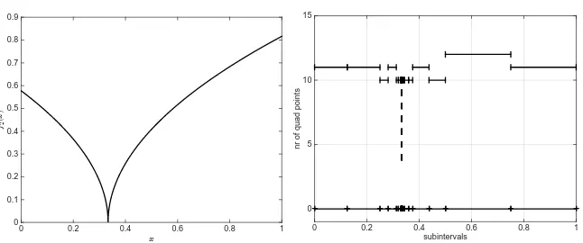
Whilst the first function, f1, is analytic, f2is smooth except at1/3(see Figure 1). Furthermore, f3was proposed in [9] in the context of theCHEBFUNpackage [10]; this is a smooth function that exhibits several very thin spikes (see Figure 2). More-over, f4is highly oscillating towards the right end point 1, and f5is an example of a discontinuous function.

We perform our computations in MATLAB, and set the tolerance to tol= 0.3×10−15 (which is close to machine precision in MATLAB), the smoothness estimation parameter is prescribed asτ =0.6, pmin=2, and pmax=15. Within this setting, our adaptive procedure generates results that are accurate to machine precision, for all of the considered examples. In Table 1, for each of the func-tions f1, . . . ,f5above, we present the number of function evaluations (counting an evaluation of the given function fi for a vector-valued argument xxx= (x1, . . . ,xn), i.e.,fi(xxx) = (fi(x1), . . . ,fi(xn)), asn) for the proposedhp-adaptive quadrature proce-dure, as well as the corresponding number for a classical adaptive Simpson method from [7] (which is based on employing the two end points, as well as the midpoint on each subinterval, and reuses the former two points without recomputing), with the same tolerance valuetol=0.3×10−15. Except for the last function, f5, where a low-order quadrature rule is more effective, the remarkable efficiency of the pro-posedhp-type quadrature becomes clearly visible.

un-x

0 0.2 0.4 0.6 0.8 1

f2

(

x

)

0 0.1 0.2 0.3 0.4 0.5 0.6 0.7 0.8 0.9

subintervals

0 0.2 0.4 0.6 0.8 1

nr of quad points

0 5 10 15

Fig. 1 Functionf2: Graph (left) andhp-mesh (right).

x

0 0.2 0.4 0.6 0.8 1

f3

(

x

)

0 0.2 0.4 0.6 0.8 1 1.2

subintervals

0 0.2 0.4 0.6 0.8 1

nr of quad points

0 2 4 6 8 10 12 14 16

Fig. 2 Functionf3: Graph (left) andhp-mesh (right).

derlying integrand are resolved by employing larger subintervals featuring a higher number of quadrature points, whereas close to singularities, the number of quadra-ture points is kept low on very small integration subdomains. It is noteworthy that this behaviour is well-known fromhp-FEMs for differential equations, where high-order algebraic or even exponential convergence rates can be obtained by applying this type ofhp-refinement procedure; see [18] for details.

3 Conclusions

Since our approach is closely related to thehp-FEM technique, it can be extended to multiple dimensions, including, in particular, the application of anisotropic refine-ments of the underlying domain of integration, together with the exploitation of dif-ferent numbers of quadrature points in each coordinate direction on each subinterval (based, for example, on anisotropic Sobolev embeddings as outlined in [6,§3.1]).

References

1. I. Bogaert, Iteration-free computation of Gauss-Legendre quadrature nodes and weights, SIAM J. Sci. Comput.36(2014), no. 3, A1008–A1026. MR 3209728

2. G. Dahlquist and ˚A. Bj¨orck,Numerical methods in scientific computing. Vol. I, Society for Industrial and Applied Mathematics (SIAM), Philadelphia, PA, 2008.

3. P. J. Davis and P. Rabinowitz,Methods of numerical integration, Dover Publications, Inc., Mineola, NY, 2007, Corrected reprint of the second (1984) edition.

4. L. Demkowicz,Computing with hp-adaptive finite elements. Vol. 1, Chapman & Hall/CRC Applied Mathematics and Nonlinear Science Series, Chapman & Hall/CRC, Boca Raton, FL, 2007, One and two dimensional elliptic and Maxwell problems.

5. R. DeVore and K. Scherer,Variable knot, variable degree spline approximation to xβ_, Quan-titative approximation (Proc. Internat. Sympos., Bonn, 1979), Academic Press, New York-London, 1980, pp. 121–131.

6. T. Fankhauser, T. P. Wihler, and M. Wirz,The hp-adaptive FEM based on continuous Sobolev embeddings: isotropic refinements, Comput. Math. Appl.67(2014), no. 4, 854–868. 7. W. Gander and W. Gautschi,Adaptive quadrature—revisited, BIT40(2000), no. 1, 84–101. 8. W. Gui and I. Babuˇska,The h, p and h−p versions of the finite element method in

one-dimension, parts I–III, Numer. Math.49(1986), no. 6, 577–683.

9. N. Hale,Spike integral, 2010, http://www.chebfun.org/examples/quad/SpikeIntegral.html. 10. N. Hale and L. N. Trefethen,Chebfun and numerical quadrature, Sci. China Math.55(2012),

no. 9, 1749–1760.

11. P. Houston and E. S¨uli,A note on the design of hp–adaptive finite element methods for elliptic partial differential equations, Comput. Methods Appl. Mech. Engrg.194(2-5)(2005), 229– 243.

12. J. M. Melenk and B. I. Wohlmuth,On residual-based a posteriori error estimation in hp-FEM, Adv. Comp. Math.15(2001), 311–331.

13. W. F. Mitchell and M. A. McClain,A comparison of hp-adaptive strategies for elliptic partial differential equations, ACM Trans. Math. Softw.41(2014), 2:1–2:39.

14. W. H. Press, S. A. Teukolsky, W. T. Vetterling, and B. P. Flannery,Numerical recipes, third ed., Cambridge University Press, Cambridge, 2007, The art of scientific computing. 15. K. Scherer,On optimal global error bounds obtained by scaled local error estimates, Numer.

Math.36(1980/81), no. 2, 151–176.

16. D. Sch¨otzau, C. Schwab, and T. P. Wihler,hp-DGFEM for second-order mixed elliptic prob-lems in polyhedra, Math. Comp. (in press).

17. C. Schwab,Variable order composite quadrature of singular and nearly singular integrals, Computing53(1994), no. 2, 173–194. MR 1300776 (96a:65035)

18. C. Schwab,p- and hp-FEM – Theory and application to solid and fluid mechanics, Oxford University Press, Oxford, 1998.

19. L. F. Shampine,Vectorized adaptive quadrature in Matlab, J. Comput. Appl. Math. 211 (2008), no. 2, 131–140.

20. P. Solin, K. Segeth, and I. Dolezel,Higher-order finite element methods, Studies in advanced mathematics, Chapman & Hall/CRC, Boca Raton, London, 2004.