Energy efficient sparse connectivity from imbalanced synaptic plasticity rules

Energy Efficient Sparse Connectivity from

Imbalanced Synaptic Plasticity Rules

João Sacramento*1, Andreas Wichert1, Mark C. W. van Rossum2

1INESC-ID & Instituto Superior Técnico, Universidade de Lisboa, Porto Salvo, Portugal,2Institute for Adaptive and Neural Computation, School of Informatics, University of Edinburgh, Edinburgh, United Kingdom

*[email protected]

Abstract

It is believed that energy efficiency is an important constraint in brain evolution. As synaptic transmission dominates energy consumption, energy can be saved by ensuring that only a few synapses are active. It is therefore likely that the formation of sparse codes and sparse connectivity are fundamental objectives of synaptic plasticity. In this work we study how sparse connectivity can result from a synaptic learning rule of excitatory synapses. Informa-tion is maximised when potentiaInforma-tion and depression are balanced according to the mean presynaptic activity level and the resulting fraction of zero-weight synapses is around 50%. However, an imbalance towards depression increases the fraction of zero-weight synapses without significantly affecting performance. We show that imbalanced plasticity corresponds to imposing a regularising constraint on theL1-norm of the synaptic weight vector, a proce-dure that is well-known to induce sparseness. Imbalanced plasticity is biophysically plausi-ble and leads to more efficient synaptic configurations than a previously suggested

approach that prunes synapses after learning. Our framework gives a novel interpretation to the high fraction of silent synapses found in brain regions like the cerebellum.

Author Summary

Recent estimates point out that a large part of the energetic budget of the mammalian cor-tex is spent in transmitting signals between neurons across synapses. Despite this, studies of learning and memory do not usually take energy efficiency into account. In this work we address the canonical computational problem of storing memories with synaptic plas-ticity. However, instead of optimising solely for information capacity, we search for energy efficient solutions. This implies that the number of functional synapses needs to be small (sparse connectivity) while maintaining high information. We suggest imbalanced plastici-ty, a learning regime where net depression is stronger than potentiation, as a simple and plausible means to learn more efficient neural circuits. Our framework gives a novel inter-pretation to the high fraction of silent synapses found in brain regions like the cerebellum.

a11111

OPEN ACCESS

Citation:Sacramento J, Wichert A, van Rossum MCW (2015) Energy Efficient Sparse Connectivity from Imbalanced Synaptic Plasticity Rules. PLoS Comput Biol 11(6): e1004265. doi:10.1371/journal. pcbi.1004265

Editor:Peter E. Latham, University College London, UNITED KINGDOM

Received:April 19, 2014

Accepted:April 5, 2015

Published:June 5, 2015

Copyright:© 2015 Sacramento et al. This is an open access article distributed under the terms of the Creative Commons Attribution License, which permits unrestricted use, distribution, and reproduction in any medium, provided the original author and source are credited.

Data Availability Statement:All relevant data are within the paper.

Funding:This work was supported by national funds through Fundação para a Ciência e a Tecnologia (FCT) with reference UID/CEC/50021/2013 and two individual grants awarded to JS with references SFRH/BD/66398/2009 and Incentivo/EEI/LA0021/ 2014. The funders had no role in study design, data collection and analysis, decision to publish, or preparation of the manuscript.

Introduction

The brain is not only a very powerful device, but it also has remarkable energy efficiency com-pared to computers [1]. It has been estimated that most of the energy used by the brain is asso-ciated to synaptic transmission [2]. Therefore to minimise energy consumption, the number of active synapses should be as low as possible while maintaining computational power [1,3,4]. The number of active synapses is the product of the activity and the number of synapses. Ener-gy can thus be reduced in two ways: 1) by employing asparse neural code, in which only few neurons are active at any time, 2) by removing synapses leading tosparse connectivity, leaving only few synapses out of many potential ones. This latter process is also called dilution of the connectivity. Remarkably, during human development brain metabolism neatly tracks synapse density, rapidly increasing after birth followed by a reduction into adolescence (e.g. compare the data in [5] to [6]).

Most computational algorithms of learning, however, optimise storage capacity without tak-ing energy efficiency into account (but see [3]) and as a result only limited agreement between models and experimental data can be expected. The best studied artificial example of learning is the perceptron which learns to classify two sets of input patterns. Despite its simplicity, re-sults of perceptron learning are crucial as they for instance guide the design of recurrent at-tractor networks [7–9]. Provided the task can be learned, the perceptron learning rule is guaranteed to find the correct synaptic weights. The traditional perceptron learning algorithm assumes that weights can have any value and can change sign. In that case a perceptron withN

synapses can on average learn 2Nrandom patterns. At the maximum load the corresponding weight distribution is Gaussian, i.e., the connectivity is dense and hence energy inefficient [10]. If one restricts the synapses to be excitatory, the capacity is halved [9,11].

In this work we ask which learning algorithm maximises energy efficient storage, and thus maximises the number of silent synapses while still being able to perform a learning task [3]. However, finding the weight configuration with the fewest possible (non-zero) synapses is a combinatorialL0-norm minimisation task. This is in general a NP-hard problem [12,13] and

thus difficult to solve exactly. Using the replica method from statistical mechanics it is possible to calculate limits on the achievable memory performance with a fixed number of synapses [10], but such methods do not yield insight on how to accomplish this. An earlier approach prunes the smallest synapses after learning. If synapses are to be removed after learning, this procedure is optimal [14,15]. Yet, as we will show it is far better to incorporate a sparse con-nectivity objective during the learning process.

Here we explore imbalanced plasticity as a simple and biologically plausible way to reduce the number of required synapses and thus improve information storage efficiency. In many memory models the amount of potentiation and depression are precisely matched to the statis-tics of the neural activity [16–19], but here we deliberately perturb the optimal plasticity rule by introducing a bias towards depression. This imbalanced plasticity finds weight configura-tions that require less functional synapses and that are thus more energy efficient.

Results

The model

We consider a recognition task from positive examples [20–22]. The perceptron should learn to give a response whenever a sample from a given category is presented. In contrast to the standard perceptron algorithm, which‘unlearns patterns’for which the neuron should not be active, the synapses are not modified for negative samples. It has been argued that this setup is relevant to biology in particular when the set of negative samples is very large and/or its

statistics unknown [22]. For instance, one might want to train a neuron to recognise fruits, but not update the synapses for all other objects. This setup is also relevant when studying rein-forcement learning, where learning is gated by reward feedback elicited by positive samples. Fi-nally, it resembles the one-class support vector machine used in statistical learning, which detects whether a sample belongs to a class and which has applications in anomaly detection [23,24].

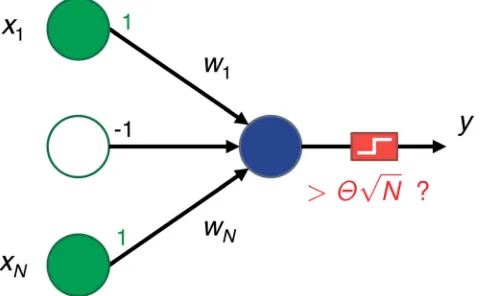
The setup is illustrated inFig 1. A single postsynaptic neuron calculates the weighted sum of itsNexcitatory inputs and compares it to a positive thresholdypffiffiffiffiN. Wheneverh¼

PN

i¼1wixiy ffiffiffiffi

N

p

is non-negative, the perceptron fires. The inputsxiare randomly chosen to

be -1 or +1 with equal probability, and independently of the other inputs (see below for exten-sions). ThepffiffiffiffiNin the threshold is a mathematical convenience that ensures scaling of the sys-tem as the number of inputs is varied [11,25].

During learning the neuron is provided with a set ofKpositive patterns,x1,. . .,xk,. . .,xK. As in the standard perceptron, we cycle through the set of patterns until the task is learned. The goal of the perceptron is to‘fire’for all these patterns. This should be contrasted to setups in which samples are presented only once (one-shot learning), which generally lead to a lower capacity [25]. We assume that initially all weightswiare zero (tabula rasa). The learning rule is

as follows: whenever a positive pattern is presented and only if it does not lead to postsynaptic activity, the synapse is updated. For high inputs, i.e.,xi= 1, potentiation occurs

Dwþ_i ¼a½1YðhÞ; ð1Þ

whereΘ() is the Heaviside step function which is zero if its argument is negative and one oth-erwise, anda1 is the potentiation rate. Similarly, when an inputxiis low, the synapse

de-presses

Dw_i ¼ b½1YðhÞ; ð2Þ

wherebis the amount of depression. Depression is followed by rectification so that all synapses remain excitatory,wi0 [26–30]. If the pattern does already lead tofiring of the perceptron,

Fig 1. Diagram of our single neuron setup.A group ofNinput presynaptic neurons are connected to a single postsynaptic neuron. The input activity can be low,xi=−1, or high,xi= 1. The postsynaptic neuron

performs a weighted sum of the inputs and fires whenever that sum is larger than a thresholdypffiffiffiffiN, otherwise it remains quiet. Each synapsewiis adjusted as a function of the input activity so that the neuron remembers

a set of previously seen patterns. Ideally, only these patterns should trigger the neuron; all other patterns should not.

no synapse is altered. This stop-learning condition is also present in a standard perceptron; possible biophysical mechanisms are discussed in [31].

For the simple, random pattern statistics used here, the non-negativity constraint limits the maximal amount of patterns that can be learned toKmax=N[9,11], which is half of the

num-ber of patterns an unconstrained perceptron can learn. Below this limit the learning process finishes with high probability in a number of steps that is polynomial inN. We define the memory loadα=K/N, which becomesαmax= 1 at the maximal load in the balanced case.

Imbalancing plasticity promotes sparseness

Unlike the traditional perceptron rule, we allow for distinct amounts of potentiation and de-pression. By introducing imbalance in favour of depression the learning dynamics is biased to-wards the hard bound of the weight at zero. We rewrite the plasticity rule using the learning rateε(a+b)/2 and an imbalance parameterλ(b−a)/2ε. Provided the synapse does not hit the zero bound, the weight update is

Dwi¼½1YðhÞðxilÞ: ð3Þ

The parameterλis zero for balanced learning; depression is stronger than potentiation if 0<λ1. Wefind somewhat improved faster learning when we also depress even when the pattern has already been learned, i.e.

Dwi ¼f½1YðhÞðxilÞ YðhÞlg: ð4Þ

For that case it can be shown that the learning dynamics minimises the energy function

E¼X

K

k¼1

ypffiffiffiffiNX

N

i¼1 wix

k i

" #

þ

þlX

N

i¼1

wi; ð5Þ

where []+denotes rectification. Thefirst term of the energy sums over all patterns and

pro-motes low false negative rates; it is zero if the perceptronfires, while it attributes a cost propor-tional to the distance to thefiring threshold whenever a pattern is not yet learned. The second term acts as a linear regulariser; the depression-potentiation imbalanceλpenalises synaptic weight configurations that have large linear normsjwj PN_i¼1wi. The regularisation term has

a simple interpretation, as it is proportional to the mean synaptic weight,jwj=Nhwi. The plas-ticity rule,Eq 4, minimises this energy by performing a stochastic sub-gradient descent [32], projected onto the subspace {w:wi0,i= 1,. . .,N}.

Rewriting the learning rule as the minimisation of the energyEq (5)shows explicitly why introducing imbalance towards depression promotes weight sparseness. In linear regression and classification, optimising over regularised energy functions that penalise theL1-norm kwk₁ PN

i¼1jwijof the weights is well-known to induce sparseness [33–35]. Below the critical

loadαmaxthe weight configuration with minimal linear norm is known to be sparse [27]. Thus,

the learning ruleEq (4)with imbalanceλ>0 will try to find solutions that satisfy the learning conditions but that are sparser than those obtained whenλ= 0.

While the linear norm constraint promotes sparseness, it is not guaranteed to produce the sparsest possible solution. The true optimisation problem would be to minimise theL0

-pseu-do-normjjwjj0. TheL0-pseudo-norm simply counts the number of non-zero synapses.

Howev-er, this leads to a difficult NP-hard combinatorial optimisation task [12,13]. Instead, optimising under theL1-norm constraint is a convex relaxation of the original problem for

which efficient computer algorithms exist (e.g. [36]). Moreover, imbalancing plasticity has the

advantage of being an online procedure that only requires tuning the potentiation and depres-sion event sizes and is thus biologically plausible.

Information and efficiency

Ideally our perceptron learns all examples, and minimises the false positive rate. To character-ise the performance we present the perceptron with learned samples and lures (other random patterns), both presented with equal probability. The mutual information between the class of the input pattern and the perceptron’s output on a given trial is

I¼ X

x2fp;lg X

r¼0;1

PðxÞPðrjxÞlog2

PðrjxÞ

PðrÞ ; ð6Þ

where P(x) = 1/2 is the probability that the test pattern is a positive pattern (p) or negative lure pattern (l), P(r) is the probability that the perceptron remains silent orfires, and P(rjx) is the conditional probability that we observe a given response given the true pattern class.

The information can be expressed in terms of the false positive ratep01and the false

nega-tive ratep10. Below the critical capacity (ααmax), the positive samples are recognised

perfect-ly after learning, i.e. there are no false negatives (p10= 0), so that the information is determined

by the false positive rate only. As we have 2Ktrials, the total information normalised per syn-apse,C¼2K

N I, equals

C¼2K N 1

1 2 h

ð1þp01Þlog2ð1þp01Þ p01log2p01

i

: ð7Þ

Although this type of information calculation is common, we note that testing with equiproba-ble lures and learned patterns is somewhat sub-optimal in terms of information [37]. For the one-class perceptron, testing exhaustively with all 2N−Kpossible lures gives about 60.6% more information whenp01= 1/2 with a weak dependence onp01.

As the mutual information does not take energy efficiency into account, we consider a re-cently suggested capacity measure that includes the sparseness of the final weight configuration [3]. Thememory efficiency Smeasures the information per non-zero synapse by normalising the information to the fraction of non-zero synapsesF,

S¼C

F: ð8Þ

Memory efficiency is thus measured inbits per functional synapse. Learning rules that achieve high informationCusing few resources will have high efficiency. If one assumes that a non-zero synapse has a certain energy cost (independent of synaptic weight) and a non-zero synapse has none, the memory efficiencySmeasures the energy cost of the stored memory.

Imbalanced plasticity improves memory efficiency

A variant of the sign-constrained perceptron convergence theorem (seeMethods) shows that the learning algorithmEq 3converges below a critical imbalanceλmax(α) that depends on the

memory loadα. In computer simulations we focus on the two extreme cases, i.e., balanced (λ= 0) and maximally-imbalancedλ=λmax(α) plasticity. In principle it is possible to find the

For strongest depression (λ=λmax), the informationCis only slightly below the information

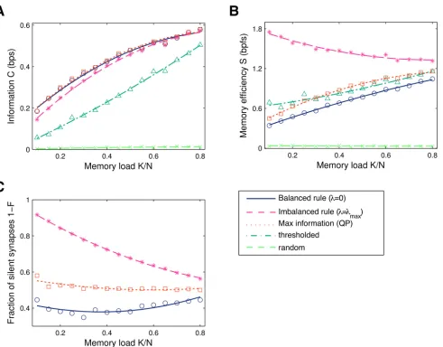
of balanced learning,Fig 2A(magenta vs. blue curve). However, imbalanced plasticity provides a large increase in memory efficiencyS,Fig 2B. The reason is that the learning dynamics con-verges to synaptic configurations with a considerably larger number of silent synapses,Fig 2C. As the memory loadαincreases, the efficiency approaches that of the balanced solution. This is expected; by increasing the task difficulty we are imposing additional constraints on the

Fig 2. InformationCin bits per synapse (bps), memory efficiencySin bits per functional synapse (bpfs) and the fraction of silent synapses 1−Fas a function of the memory load_α=_K/_N.Results from a simulation with_N= 1000 synapses. Shown are: balanced learning where depression equals potentiation (λ= 0); maximal imbalance learning; the maximal-information solution found with offline quadratic programming (QP); minimal-value synapse deletion, where all weights below some threshold are set to zero; and random pruning. The two latter rules were set to delete the same number of synapses as imbalanced learning. The results for online learning were obtained under a large threshold (θ= 1, learning rateε= 1/N) to maximise information (see Methods).A. Information. Imbalanced plasticity leads to a small information decrease and significantly outperforms thresholded pruning. Random deletion performs very poorly. Truly maximising information (QP) gives only a slight improvement in performance.B. Memory efficiency (information per non-zero synapse). In particular at lowα, the imbalanced perceptron finds sparser weight configurations, boosting the memory efficiency. The curves converge as the critical loadingα= 1 is approached. The maximal information solution (QP) is more efficient than balanced learning, but still inferior to imbalanced learning.C. The fraction of silent synapses. Balanced online learning (_λ= 0) under a large threshold always leads to the appearance of silent synapses, due to the imposed hard bound at zero together with the large firing threshold. Imbalanced plasticity significantly increases sparseness, especially at lower memory loads. QP learning leads to a few more zero-weight synapses compared to balanced learning, the fraction of which remains close to 50% irrespectively of the memory load.

doi:10.1371/journal.pcbi.1004265.g002

synaptic weights. As a result the volume of the solution space shrinks and the constraint on the mean weight has to be relieved, therefore leading to smaller gains in memory efficiency. Asα approaches its critical value, the space of solutions collapses to a single point, i.e., no additional constraints can be imposed at critical capacity andλmax= 0 [7].

We also considered alternative learning algorithms: first, a minimal-value pruning rule, where all weights below a certain threshold are set to zero after learning has converged. We set the deletion threshold of the offline pruning algorithm to produce the same number of zero-weight synapses as the imbalanced solution. This is optimal in the one-shot learning case [14, 15]. In this case we find a more pronounced loss of information and, interestingly, almost no efficiency increase (dark green curve). The superiority of imbalancing makes intuitive sense: imbalanced plasticity is an online protocol that accommodates for sparseness constraints by re-distributing weights dynamically, while the pruning procedure is performed after learning and does not allow for further re-adjustments. Finally, we also tried random pruning after learning, which as expected, performs very poorly (light green curve).

For completeness, we compared these results to the solution that maximises information without requiring sparseness. The optimisation can be formulated as a quadratic programming (QP) problem (seeMethods), and the best solution can be found with a high performance bar-rier method convex optimiser [38]. This algorithm clearly lacks biological plausibility, and does not provide a significant improvement in information over balanced (λ= 0) online learn-ing,Fig 2A. In other words, perceptron learning works well for our problem, provided that the firing thresholdθis large enough (seeMethods). Under QP the fraction of silent synapses slightly increases to around 50%,Fig 2C, which leads to a moderate improvement in memory efficiency,Fig 2B. Finally, one can resort to the min-over learning rule, which only applies a weight update for the pattern that evokes the minimal outputh[39]. The synaptic weights are guaranteed to asymptotically converge (asθ! 1) to the QP solution and unsurprisingly the information matches that which is obtained with the quadratic solver. This procedure is diffi-cult to reconcile with biology as well, as each single learning iteration requires access to every pattern.

Synaptic weight distributions

The learning algorithm and the threshold setting also determine the shape of the synaptic weight distribution. This distribution is of importance, as it can be compared to experimental data. For instance, the electro-physiologically determined synaptic weight distribution was used to link Purkinje cell learning to perceptron learning theory [28,40]. We recorded the ob-tained synaptic weight histograms (seeMethods), averaged over many trials (each with differ-ent pattern sets). While collecting results across trials is strictly only approximates the synaptic weight density, it is a good estimate of the actual observed distribution for a single realisation of the system, since the underlying weight density is strongly self-averaging [27,28].

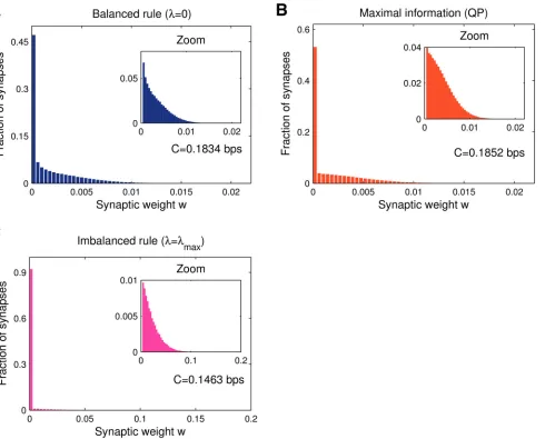
Balanced learning (λ= 0) leads to an approximately exponential distribution,Fig 3A. Inter-estingly, although the QP solution did not increase information compared to online balanced learning (Fig 2A), the shape of the distribution of synaptic weights changes considerably (cf. Fig3Aand3B). At any memory loadααmaxthe fraction of zero-weight synapses always

re-mains close to 50% while the remaining weights assume a truncated Gaussian distribution cen-tred aroundw= 0. The problem that we are dealing with is thus not‘intrinsically sparse’in weight space. This should be contrasted with the non-negative perceptron classifier with 0/1-coded inputs that was recently studied [28–30]. In that case, maximising information in the presence of postsynaptic noise automatically leads to sparse weight configurations

load, the distribution becomes identical to the truncated Gaussian that we report here as the optimal one.

Imbalanced plasticity boosts the fraction of zero-weight synapses and stretches the weight distribution,Fig 3C. Although the mean weight is lower due to the increased sparseness of the weight configuration, the surviving synapses are stronger. This can be understood through the-oretical arguments (seeMethods). It can be shown that learning rules that lead to a large

mini-mum postsynaptic sum,mink

PN

i¼1wixki (together with a normalisation condition that fixes the

Euclidean normjjwjj2) give better recognition performance against lures. As some synapses are

zeroed-out, specific strengthening keeps the postsynaptic sum large for learned patterns.

Fig 3. Synaptic weight histograms, information and memory efficiency at low memory load (_α= 0.1).Data obtained averaging over a thousand simulations (N= 1000).A. For balanced learning the distribution is stretched due to the optimised learning (large threshold choiceθ= 1 under a small learning rateε= 1/N). As with the non-negative perceptron classifier [28], a large number of zero synapses appear.B. Maximal-information solution obtained via quadratic programming, with the objective set at minimising the Euclidean normjjwjj2. The quadratic objective function leads to a hemi-Gaussian weight

distribution, again with a large fraction of silent synapses arising from the non-negativity constraint.C. Minimal linear norm solution (largest imbalance). As the learning task is‘easy’(lowα), strong depression leads to a highly sparse synaptic configuration.

doi:10.1371/journal.pcbi.1004265.g003

The non-zero weight distribution for maximal imbalance can be reasonably fitted to a com-pressed exponentialP(w)*exp(−cwβ), with an exponentβ= 1.4. The two-class perceptron model yieldsβ= 2 (a truncated Gaussian) at critical capacity [28]. The best fit of this type of distribution to the cerebellar data published [40] has an exponentβ= 0.7±0.4, however it should be noted that the limited amount of data allows for a broad range of possibleβ.

Homeostatic excitability regulation and sparse codes

Next we explore if our findings depend on the details of the coding. So far we assumed the in-puts were -1 or +1, as in earlier studies of the non-negative perceptron [9,26,27]. This is hard to imagine biologically, unless an inhibitory partner neuron is introduced [19,31,41,42]. An arguably more faithful biological model is obtained by representing low inputs as silent,xi= 0

[16,19,20,28,43]. Furthermore, we wish to generalise to a case where the probability for a high input is variable rather than fixed to 1/2.

The capacity of the above model can be fully recovered without drastically changing the neural circuit. In fact, two ingredients suffice: one has to rebalance the plasticity rules as a func-tion of the activity levelf, and, secondly, introduce a dynamic mechanism that adapts the firing threshold as a function of the linear normjwj. With these modifications, both the information

Cand the memory efficiencySare exactly identical to those reported in the previous section. First, we generalise the model to deal with an arbitrary coding levelf. Whenf= 1/2, the orig-inal model is recovered up to scale factors. To preserve the zero mean, we consider activity pat-terns that are coded aszi2{−f,1−f}, with P(zi= 1−f) =f. Stochastic sub-gradient descent

dynamics over the energyEq (5)gives the adjusted potentiation rule for high inputs

Dwþ

i ¼fð1f lÞ½1YðhÞ lYðhÞg; ð9Þ

while depression at low inputs becomes

Dw_i ¼fðf þlÞ½₁YðhÞ lYðhÞg; ð10Þ

followed by rectification. Hereh¼PNi¼1wiziy ffiffiffiffiffi

fN

p .

Next, a zero-mean inputziis related to 0/1 coding by the simple relationxi=zi+f,xi2{0,1}.

Therefore the net input of the neuron in response to a 0/1 pattern can be written through a change of variables as

h¼X

N

i¼1 wixif

XN

i¼1 wiy

ffiffiffiffiffi

fN

p

¼X

N

i¼1

wixig; ð11Þ

where we defined a new threshold variable

g¼fX

N

i¼1 wiþy

ffiffiffiffiffi

fN

p

:

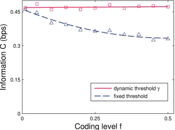
of the input coding levelf(Fig 4solid line), while it decreases when the threshold isfixed (dashed curve). We note that, unlike for two-class learning, for one-class learning a high threshold suffices to implement a large-margin classifier.

An alternative route to recover capacity is to employ sparse coding, a finding that has been previously reported for the non-negative perceptron in a more general classification framework [43]. Here the asymptotic situation is rather simple, because asf!0 andN! 1the original model is recovered and performance at lowfapproaches the ideal performance,Fig 4.

Input correlations

Activity correlations can severely limit the performance of learning rules, depending on the task and the nature of the correlations. For instance, in supervised memory tasks, Hebbian learning deteriorates under almost any type of correlation in the patterns [25,44]. In contrast, more powerful plasticity rules equipped with a stop-learning condition, like the perceptron rule, are resistant to spatial input correlations [45], and can in some cases take advantage of input-output redundancies to store more patterns [29,46].

To test the robustness of imbalanced plasticity to correlated activity we draw random pat-terns from a generative model that induces spatial presynaptic activity correlations (character-ised by a parameterg, seeMethods, [21,45]). We first correlated the patterns such that the

Fig 4. InformationCin bits per synapse for binary (0 or 1) input patterns as a function of the input coding levelf.Average values for the dynamic-threshold model, wherehis given byEq 11, and average values obtained with a fixed thresholdθfN—note the threshold scaling withfNinstead ofpffiffiffiffiffifNdue to the 0/1 input activity. Potentiation and depression were balanced (Eqs9and10) to match the coding level. While the adjusted model is insensitive tof, the information achieved by the uncorrected model approaches that of the original one for sparse input patterns. Simulations performed at moderate memory load_α= 0.5 and system sizeN= 1000.

doi:10.1371/journal.pcbi.1004265.g004

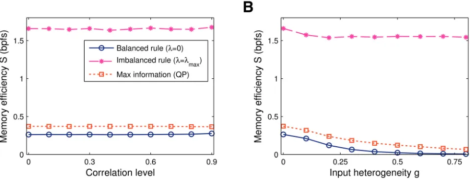
mean activity remained homogeneous across the inputs. Consistent with the standard two-class perceptron without synaptic sign-constraints [45], neither the imbalanced learning, nor the balanced rule are affected by input correlation,Fig 5A.

Next, we implemented a variation of the generative model that introduces heterogeneities in the input activity rates where some inputs tend to be active more often than others. Interesting-ly the imbalanced rule is robust to this type of correlation,Fig 5B. Whereas the efficiency of the other rules drops off, the efficiency of the imbalanced rule remains constant. The intuitive ex-planation is that the high activity synapses effectively experience balanced net potentiation and depression for non-zero imbalanceλ. The imbalanced rule finds a high-information solution by silencing and ignoring the low activity inputs and subjecting the remaining synapses to the usual imbalanced learning protocol.

Robustness to noise

So far we have considered the recall of noise-free patterns, however, in the light of the many noise sources in the nervous system, it is important to confirm the noise robustness of the results.

First, we introduce transmission failures and spontaneous presynaptic activity, and test the learning with corrupted patterns, denotedx~. An active input is switched off with probability

d₁₀¼Pð~xi¼0jxi¼1Þ, while an otherwise silent presynaptic input fires with probability

d₀₁¼Pð~xi¼1jxi¼0Þ. The lures are generated with a matching mean activity,hxi= (1−f)δ01+f

(1−δ10), to ensure that lure statistics match the patterns.

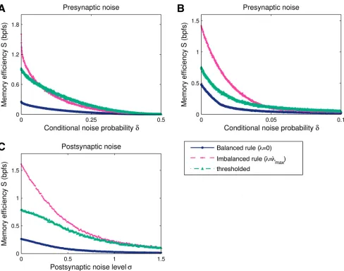
We examined the performance of the balanced and maximally-imbalanced rules, as well as thresholded synaptic pruning, under this stochastic synapse model, Fig6Aand6B. The infor-mation of all three rules decreases smoothly as the input distortion increases. For dense pat-terns,f= 1/2, the efficiency of the maximally-imbalanced rule is initially the most affected by the introduction of noise, and becomes comparable to the thresholded deletion one for higher

Fig 5. Memory efficiency vs input correlations. A. In case the mean input remains homogeneous, the three learning algorithms considered_—balanced (λ= 0), maximally-imbalanced (λ=λmax) and maximal-information (QP)—are unaffected by spatial presynaptic activity correlations.B. In case of heterogenous

inputs, the balanced rule (λ= 0) and the QP algorithm deteriorate. Imbalanced plasticity performs well, however, as it regularises the high-activity synapses while ignoring the remaining ones. As a result the memory efficiency of the maximally-imbalanced solution is approximately constant. Data obtained by averaging a hundred independent simulations at_α= 0.1,_f= 1/2, and_N= 1000 synapses.

noise levels. For sparse patterns,Fig 6B, the efficiency is affected similarly by the noise for all three rules. The maximally-imbalanced and the thresholded solutions remain more efficient than balanced plasticity.

Next, we examined the role of postsynaptic current noise by adding a zero-mean Gaussian variable to the postsynaptic currenth[28], the variance of which sets the noise intensity,Fig 6C. In contrast to the above, the magnitude of the random contributions is decoupled from the actual learned weights. For this noise model, the relative information reduction is comparable for both balanced and imbalanced plasticity.

Fig 6. InformationCand memory efficiencySversus noise level.The three solutions—balanced (λ= 0) and maximally-imbalanced (λ=λmax) plasticity,

and thresholded synaptic pruning_—were obtained once for a single set of_K= 0.1_Npositive patterns (_N= 1000 synapses) and then tested against a large number 100Kof distorted learned patterns and lures, generated for each noise level. The firing threshold of each solution is numerically optimised to maximise information. The presynaptic noise level varied under the settingδ01=δ10=δ(see main text for details). The scale of the postsynaptic noise

standard deviation was set by normalising the weights to give a unit size mean response to learned patterns.A. For dense patterns,f= 1/2, the falloff in information is steeper for imbalanced plasticity than thresholded deletion. The two solutions remain more efficient than balanced learning for all noise levels. B. For sparse input patterns,f= 0.01, the balanced solution also suffers and as long as the information is not practically zero, both the maximally-imbalanced and the thresholded pruning rules are more efficient than the balanced one.C. Results for a postsynaptic noise model, where the currenthis perturbed with an additive zero-mean Gaussian random variable with standard deviationσ. As the postsynaptic noise does not depend on the actual learned weights, imbalanced and balanced plasticity show similar noise robustness profiles.

doi:10.1371/journal.pcbi.1004265.g006

Tuning of the imbalance parameter

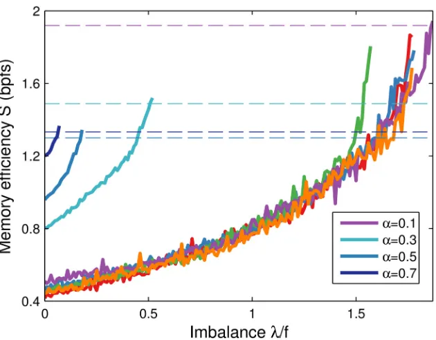
In the above the imbalance parameterλwas optimised for automatically in an unbiological fashion. To examine suboptimal values we simulated learning while raisingλtowards the criti-cal imbalanceλmax, above which the learning algorithm no longer converges. The memory task

difficulty, set by the memory loadα, limits the allowed imbalance (seeMethods). Indeed, we find thatλmaxshrinks asαincreases,Fig 7. Akin to the margin parameter which sets the noise

robustness of the non-negative perceptron [28,29], the actualλmaxdepends on the exact set of

patterns the neuron should learn. However, for random patterns drawn from the same distri-bution, the system is self-averaging asN! 1[7]. In simulations we observe a similar behav-iour across different runs, although some finite-size effects are still apparent in networks of moderate dimension,Fig 7(rightmost curves). In other words,λmaxcan be reasonably

estimat-ed independent of the precise pattern set. Finally note that the figure implies that the parameter can be set conservatively, based on the maximum number of patterns to be expected. Of course, the efficiency gain is not maximised in this case, but still better than the balanced case.

Discussion

The brain’s energy consumption is thought to be dominated by synaptic transmission [2,47, 48]. We have considered how synaptic learning rules can lead to sparse connectivity and thus to energy efficient computation. We studied a one-class perceptron problem in which a neuron learns from positive examples only. One-class learning is relevant for learning paradigms such

Fig 7. Memory efficiencySincreases with imbalanceλ.Efficiency is a function of imbalance for a given set of patterns. The curve stops when the learning dynamics no longer converges. Dashed horizontal lines indicate the corresponding efficiency values achieved by the linear programming solver (seeMethods). The results for five independent runs at_α= 0.1 (rightmost curves) are very similar, although finite-size effects are visible as the number of inputs is not particularly large. As predicted, the critical imbalanceλmaxdecreases

with the memory loadα. The learning rule only updated the synapses for patterns that did not yet lead to firing activity,Eq 3. Simulations of a neuron withN= 1000 synapses and coding levelf= 0.01.

as recognition and reinforcement learning. One-class learning is also well-known in machine learning [24,49,50]. The two-class perceptron requires sampling the space of‘negative’ pat-terns that is necessarily large under a sparse firing constraint [22] and secondly, it requires re-versing plasticity (‘unlearning’) whenever appropriate. For instance, it is unclear how can a pattern be actively unlearned under spike-timing-dependent plasticity [51]. In contrast to two-class perceptrons, negative samples in the one-two-class perceptron do not cause plasticity which leads to further energy saving as plasticity itself is an energetically costly process [52].

We imbalance potentiation and depression to achieve sparse connectivity. In other memory tasks, the information loss can be substantial for imbalanced plasticity; for instance, postsynap-tic-independent (i.e., without a stop-learning mechanism) online learning rules are severely af-fected when depression does not match potentiation [17–19]. However, here imbalance leads to a substantial energy reduction in storage as long as the task is below maximal capacity. Fur-thermore, it is robust against noise and correlated patterns. Imbalanced plasticity is not only a local and biophysically plausible mechanism, but it is also theoretically well-grounded, as it im-plementsL1-norm regularisation, which is well-known to induce sparseness [27,33,34,53].

Due to the biased drift towards zero in the learning rule, the probability of finding silent synap-ses is increased. Our learning rule reaches high information using a novel, biologically-plausi-ble adaptive threshold without the need for an inhibitory partner neuron. The learning rule is unlike a previous approach to achieve sparse connectivity in which a pruning procedure re-moves the weakest synapses after learning [14,15]. Such strategy can lead to as much weight sparseness as desired, but a significant drop in information and efficiency occurs.

Despite the large efficiency gain found, it should be noted that imbalanced plasticity proba-bly does not maximise the efficiency fully. In the limit of many synapses the replica technique from statistical mechanics can provide an estimate on the minimal number of synapses re-quired for a given performance. Extrapolation of such an analysis of the traditional perceptron without sign constraints [10], suggests that even more efficient solutions exist, although it is unclear how to obtain them via online learning. Unfortunately, the weight configuration that truly maximises memory efficiency requires resorting to an impractical and unbiological ex-haustive search method, with a search time exponential in the number of synapses. A feasible alternative is to use greedyL0-norm minimisation methods [54], that are in general not

guaran-teed to achieve the theoretical limiting weight sparseness. Preliminary simulations suggest that the efficiency in this case is not substantially higher than when minimising the linear norm, as the increased number of zero-weight synapses is offset by a steep loss in information.

We note that sparse network connectivity can arise even when energy efficiency is not ex-plicitly optimised for. Weight sparseness also emerges when maximising the information out-put of a sign-constrained classifier that is required to operate in the presence of postsynaptic noise [28,30]. The reported weight distribution displays a large fraction of silent synapses [28]. In that learning setup, depression occurs for negative examples to drive the postsynaptic poten-tial well below threshold and thus ensures that the activity of the neuron is suppressed even if noise is present.

In order to implement imbalanced learning various ingredients are needed. 1) As in the clas-sical perceptron a stop-learning condition needs to be implemented. While in the cerebellum the complex spike might fulfil this role, neuromodulatory systems have also been suggested [31]. 2) The balance parameter needs to be precisely set to obtain the most efficient solution and its value depends on the task to be learned. A conservative imbalance setting will increase efficiency, but not as much. We note that the need for precisely tuned parameters is common in this type of studies, just like the standard perceptron requires a precise balance between po-tentiation and depression, which is also not trivially achieved biologically. 3) For one-class learning, plasticity only occurs when the neural output should be high but it is not (which

contrasts the model in [28], where plasticity only occurs when the input is high). A separate su-pervisory input to the neuron could achieve this. Nevertheless, despite the details of this partic-ular study the general imbalancing principle could well carry over to other systems. In

particular including precise spike-timing perceptron learning [55,56], or temporal STDP [57]. In the latter case, interestingly, energy constraints have also been used to define unsupervised learning rules.

Our study is agnostic about the precise mechanism of pruning. There is a number of bio-physical ways a synapse can be inactivated [58,59]: 1) The presynaptic neuron releases neuro-transmitter, but no receptors are present (postsynaptically silent synapse). 2) Alternatively, presynaptic release is turned off (mute synapses). Finally, 3) the synapse is anatomically pruned and thus absent altogether (although it could be recruited again [60]). The first and second would presumably allow the system to rapidly re-recruit the synapse, while the third option not only saves energy, but also reduces anatomical wiring length and volume.

It is worthwhile to ask if our model is consistent with neuroscience data. Naively, one might think that imbalance would predict that LTD would be stronger than LTP, which would con-tradict typical experimental findings. However, for sparse patterns LTD has to be weakened to prevent saturation, so that the imbalance condition becomesfLTP<(1−f)LTD. It is unclear whether this condition is fulfilled in biology. Next, one could expect that the theory would pre-dict a net decrease of synaptic strength during learning. However, this is not the case: after all, in the simulations all weights are zero initially, so that synaptic weights can only grow during learning. The reason for this apparent paradox is that learning is gated, unlike unsupervised learning, so the number of LTP and LTD events on a synapse does not necessarily match. While our findings also hold when we start from random weights, there is no obvious initial value for biological synaptic weights.

Finally, one can compare the resulting weight distributions and the number of silent synap-ses to the data. An advantage of the cerebellum is that also the fraction of zero-weight synapsynap-ses is known, which is not the case for other brain regions. The weight distribution in the cerebel-lum matches theory very well when the capacity of a two-class perceptron is maximised in the presence of noise. The fraction of silent synapses exhibits a strong dependence on the required noise tolerance; it is significantly decreased in the low noise limit [28]. Our current model finds a similar distribution from a very different objective function, namely minimising the energy of a one-class perceptron. Which of these two is the appropriate objective for the cerebellum or other brain regions remains a question for future research.

Methods

Criteria for optimising information

Provided that the memory problem is realisable, perceptron learning ensures that each of theK

patterns leads to postsynaptic firing activity (h0), i.e., the FN error probability is zero,p10=

0. In this case the information increases as the FP error probabilityp01decreases (see main text,

Eq 7). With the additional assumption that the lures are uncorrelated to the learned patterns, it can be shown that our perceptron learning rule leads to a decrease of the FP error.

To see why, we writep01as a function of the learned synaptic weights. As the lure patterns

are uncorrelated to the learned ones, each inputxiwill be uncorrelated to its corresponding

weightwi. The total synaptic current is given by a sum of many terms. Assuming that there are

a lure is Gaussian,hl Nðhhli;hdh2liÞ. Under this approximation,

p01

Z 1

0

dhlpðhlÞ ¼

1 2erfc

hhli ffiffiffiffiffiffiffiffiffiffiffiffiffi 2hdh2

li p

!

; ð12Þ

whereerfcðxÞ ¼ 2ffiffi p p R1

x e

t2

dtis the complementary error function. The approximation im-proves asN! 1, as the fraction of non-zero synapsesFremainsfinite irrespective of the im-balanceλ(forλλmax) and as long as the memory loadαdoes not vanish [10].

As the inputs are in zero-mean bipolar form,hxi= 0,hx2i= 1. The mean current elicited by lures is justhhli ¼Nhxihwi y

ffiffiffiffi

N

p

¼ ypffiffiffiffiN, independent of the weights. The variance in the current

hdh2

li ¼ hðdðhlþy ffiffiffiffi

N

p ÞÞ2_{i ¼}

Nðhx2_ihw2_{i ðhxihwiÞ}2_{Þ ¼}

Nhw2_i ð₁₃Þ

is proportional to the second raw momenthw2i ¼R1

0 dw pðwÞw

2_{of the weight distribution.}

For a particular realisation of the system one hasNhw2i ¼ kwk2

2, the squared Euclidean norm

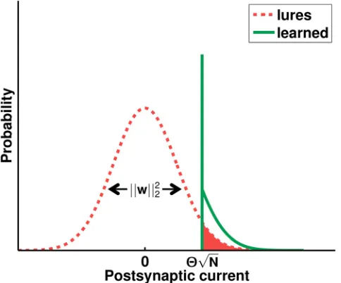
of the synaptic weight vector. This is illustrated inFig 8. The information of the system is thus given by the Euclidean norm of the weight vector alone. This is true for the learned-vs-lure dis-crimination task as long as the Gaussianity of the lure currenthlholds, irrespective of the

par-ticular learning rule that is employed. For instance,p01takes the same form for

postsynaptic-independent learning [19] or for rate-coded inputs that are learned via the offline pseudo-in-verse rule [22].

Fig 8. Schematic illustration of the postsynaptic current distributions.In the largeNlimit, the postsynaptic current elicited by lures (dashed line) is well described by a zero-mean Gaussian, whose variancehdh2

liis determined by the squared Euclidean normkwjj22of the weight vector. Assuming that the

learning dynamics converged, the postsynaptic current distribution provided that the input pattern is a learned one (solid line) is characteristic of perceptron learning: a significant number of patterns lie on the decision boundary and thus provoke a current that is exactly at the firing threshold, while the remaining ones generate super-threshold Gaussian tail currents [28]. The integral of the shaded area gives the FP probabilityp01,

which depends on the variance of the lure current distribution. doi:10.1371/journal.pcbi.1004265.g008

Thus, the perceptron with the most information satisfies the firing conditionh0 for every learned pattern, but has a minimal Euclidean length weight vector. This coincides exactly with the traditional perceptron that is optimal with respect to the maximal-stability criterion [39], that prescribes the weight configuration with largest stabilityDypffiffiffiffiN=kwk₂. This is a widely used principle that enlarges the basins of attraction in recurrent networks and improves the ability to generalise in classifiers [39,61]. Notice that for a fixed threshold, increasingΔcan only increase information, as it is inversely proportional to the Euclidean weight vector length. Information maximisation thus reveals an interesting close link between recognition memory and the more usual two-class learning problems.

Furthermore, at least for random patterns, we can expect the perceptron learning rule to perform well. Below the critical loadαmaxthe algorithm is known to converge to solutions with

largeΔ[62]. In other words, although the learning dynamics is not guaranteed to maximise in-formation, it should achieve highCin the recognition task. As shown in the main text,Fig 2, the improvement indeed is minimal when the full quadratic program is actually solved.

The crucial condition that must be observed to achieve good performance is that the firing thresholdθshould be large. Hereθplays the role of an indirect (unnormalised) stability param-eter. It can be shown [39] that raisingθwill indirectly lead to solutions with largerΔ. Lower bounds on how close the learning rule gets to maximal stability with a certain setting ofθand

a,bcan be extracted from the perceptron convergence proof [39].

Note that the above reasoning requires zero-mean inputs and balanced plasticity. For 0 or 1 inputs, the distribution of the unthresholded outputhlthat is obtained in response to lures is

still well characterised by a Gaussian, as an uncorrelated input pattern gives a sum over on av-eragefNrandomly selected weights. The expressions for the meanhhliand the variancehdh2

li

now include terms that depend on first- and second-order moments of the synaptic weight dis-tribution. For a particular realisation of the random system the mean is

hhli ¼fNhwi y ffiffiffiffi

N

p

¼fjwj ypffiffiffiffiN, and the variance

hdh2

li ¼Nðfhwi

2

f2h_wi2Þ ¼_fkwk2 2f2N

1_jwj2

. Thus, when the inputs are in 0 or 1 form, the information per synapseCis no longer a simple function of the squared Euclidean norm as before. The output error probabilityp01, and therefore the information, is affected by the

cod-ing levelfand the linear normjwjas well.

Imbalanced plasticity affects convergence of the learning dynamics

To gain further insight on the effects of allowing a depression-potentiation imbalance, we prove the convergence of perceptron learning ruleEq 3for non-zeroλ, a variation of the de-tailed proof given by [29]. Besides the inclusion of the parameterλ, differences arise because our inputs are in bipolar form and because all patterns should elicit a high output.

We study a problem that can provably be solved in a finite number of learning steps by bal-anced postsynaptic-dependent learning (λ= 0). Therefore we can assume the existence of a weight configurationwthat solves the recognition task

XN

i¼1 w_ixk

i ðyþkÞ ffiffiffiffi

N

p

0; k¼1;. . .;K; ð14Þ

while simultaneously satisfying theNnon-negativity constraintswi 0,i= 1,. . .,N. The

vari-ableκ0 relates the thresholdðyþkÞpffiffiffiffiNof the solution to the thresholdypffiffiffiffiNthat is used in the learning algorithm.

We assume that initially all synapses are silent, i.e., we start from thetabula rasacondition

only occurs when the postsynaptic currenth¼PNi¼1wixiy ffiffiffiffi

N

p

is not large enough to acti-vate the perceptron, we index time withm= 1,. . .,M,mbeing incremented only whenh<0. Whenever each synapsewichanges, it does so according to the update,Eq 3

DwiðmÞ ¼maxfwiðmÞ; ZiðmÞg; ð15Þ

whereηi(m) =xi(m)−λis the weight update before rectification andx(m)2{x1,. . .,xK} is the

pattern that led to the update at timem.

The analysis is carried out by tracking the quantity

aðmÞ ¼ w

_wðmÞ

jjw_jj

2jjwðmÞjj2

ð16Þ

over time. If wefind that after afinite number of updatesa(m) would become larger than one, then the learning process is convergent, as the Cauchy-Schwarz inequality implies that

a(m)1. To monitor the time evolution ofa(m) we bound the scalar productw w(m) from below and the normjjw(m)jj2from above.

After one update, the changeΔ(ww(m))ww(m+1)−ww(m) in the scalar product is

Dðw_{wðmÞÞ ¼ wDwðmÞ}

¼ w_{ZðmÞ þ} X

i2BðmÞ

w_iðþlwiðmÞÞ

¼ w_{xðmÞ ljwj þ} X

i2BðmÞ

w_iðþlwiðmÞÞ

> ypffiffiffiffiNþkpNffiffiffiffiljwj þ X

i2BðmÞ

w_iðþlwiðmÞÞ;

ð17Þ

whereB(m) = {i:wi(m)<ε+ελ^xi(m) =−1,i= 1,. . .,N} is the set of all synapses that are

set to zero due to the lower bound. Note that the lower bound can only be triggered by depres-sion, which in turn can only occur for low inputs. The inequality is obtained by plugging in the definitionEq (14)ofw.

A bound on the scalar productww(m) itself aftermsuch updates can then be obtained by iteratively applyingEq (17):

w_{wðmÞ> m}pffiffiffiffi_{N yþk} l_ffiffiffiffi N

p j_wj

þX

m

l¼1

X

i2BðlÞ

w_iðþlwiðlÞÞ: ð18Þ

Meanwhile, the changeDkwðmÞk2₂ kwðmþ1Þk22 kwðmÞk 2

2in the squared norm ofw

(m) after one step can be obtained by expanding the square

kwðmþ1Þk22 ¼ kwðmÞ þDwðmÞk 2 2, so that

DjjwðmÞjj22¼2wðmÞ DwðmÞ þ jjDwðmÞjj 2

2: ð19Þ

We haveΔwi(m)2{εηi(m),−wi(m)}, withwi(m)<ε+ελ, asΔwi(m) =−wi(m) only fori2

B(m). Thus, the squared norm of the update is dominated by the terms that come from low in-puts at synapses that do not cross the lower bound. This gives the inequality

jjDwðmÞjj22 < 2Nð1þ2lqþl 2

qÞ; ð20Þ

whereqmaxk1=N

PN

i¼1dxk

i;1denotes the maximum fraction of low inputs observed across

theKpatterns.

The scalar product is expanded as before:

wðmÞ DwðmÞ ¼ wðmÞ Zm_þX

i2BðmÞ

wiðmÞðþlwiðmÞÞ

¼ wðmÞ xðmÞ ljwðmÞj þ X

i2BðmÞ

wiðmÞðþlwiðmÞÞ

< wðmÞ xðmÞ þ X

i2BðmÞ

wiðmÞðþlwiðmÞÞ:

ð21Þ

Note that the update conditionh<0 is always satisfied at timem, so that

εwðmÞ xðmÞ<εypffiffiffiffiN. Together with the boundEq (20), iterating overEq (19)gives

jjwðmÞjj2₂< mN 2yffiffiffiffi N

p þð1þ2lqþl2_qÞ

þ2X

m

l¼1

X

i2BðlÞ

wiðlÞðþlwiðlÞÞ ð22Þ

< mN 2yffiffiffiffi N

p þð1þ2lqþl2_{qÞ þ}

2qð1þlÞ2

: ð23Þ

The last inequality is obtained by noticing thatwi(l)<ε+ελinside the sum overl; the factor

qarises from the iteration over theNsynapses, conditioning on the low inputs. The bound Eq (23)implies that as learning proceedsjjw(m)jj2cannot grow faster thanpffiffiffiffim.

FromEq (22)we collect

mypffiffiffiffiN>1

2

2_mNð

1þ2lqþl2_qÞ X

m

l¼1

X

i2BðlÞ

wiðlÞðþlwiðlÞÞ: ð24Þ

Turning back toEq (18)and using the previous resultEq (24)yields

w_{w > mN} k_ffiffiffiffi N

p 1

2ð1þ2lqþl

2 qÞ l

Njw _j

þXm

l¼1 X

i2BðlÞ

ðwi wiðlÞÞðþlwiðlÞÞ

> mN kffiffiffiffi

N

p 1

2ð1þ2lqþl

2 qÞ l

Njw _{j qð}

1þlÞ2

:

ð25Þ

The last inequality stems fromwi(l)<ε+ελ. Thefirst bracketed factor is always larger than

−(ε+ελ), while the second one is bounded from above byε+ελ. Iterating over the constrained sum introduces the factorNqas before.

We now have a bound for the cosinea(m). Substituting in Eqs (23) and (25) gives

aðmÞ>

ffiffiffiffiffiffiffiffiffiffi

mN

p

kN1=2_lN1jwj 1

2ð1þ2lqþl

2

qÞ qð1þlÞ2

jjw_jj 2

ffiffiffiffiffiffiffiffiffiffiffiffiffiffiffiffiffiffiffiffiffiffiffiffiffiffiffiffiffiffiffiffiffiffiffiffiffiffiffiffiffiffiffiffiffiffiffiffiffiffiffiffiffiffiffiffiffiffiffiffiffiffiffiffiffiffiffiffiffiffiffiffiffiffiffiffiffiffiffiffiffiffiffi 2yN1=2þð₁þ_2lqþ_l2_qÞ þ₂qð₁þ_lÞ2

q : ð26Þ

Note that while the neural parameters {ε,θ,λ} can be set at will, for a certain task the solution marginκand the norms are constrained by the existence of a vectorwthat can satisfy the learning conditions. Thus, they cannot be varied arbitrarily. In fact, if one keepsjjwjj2fixed, it

Furthermore, in general it is not possible to achieve simultaneously minimaljwjand maximal

κwith a single configuration.

FromEq (26)a number of conclusions can be drawn. The straightforward condition for convergence is to check whether that bound becomes larger than one. Another way to show that the learning algorithm stops is to check ifa(m) is a monotonically increasing function of

m. Whenλ= 0, the process is convergent, as long asε2k=½pNffiffiffiffið1þ2qÞ. Forλ>0, the cru-cial observation is that we can only show that learning converges ifκcan be raised so as to compensate for the negative terms in the numerator.

Thus, as expected, we find that the imbalanceλis related to the linear norm of the solution vector (one can increaseλasjwjcan be made smaller), and to the occurrence of depression events (throughq). But more importantly,λmaxwrites directly as a function ofκas well, which

here sets the task difficulty, since the maximal value forκshrinks as the memory loadα in-creases. What is more, the minimum ofjwjdepends itself onα. This theoretical prediction is confirmed by our numerical work. Asαincreases, the achievable imbalanceλmaxbecomes

clos-er to zclos-ero, and the fraction of silent synapses approaches that which is obtained with balanced (λ= 0) learning, cf.Fig 2C.

Generating correlated patterns

We generate correlated patterns following previous work in recognition memory [21]. In the first model we generate a template patternx^with each input^xibeing set high (+1) or low (-1)

independently and with equal probability 1/2. To maintain balance we also use its negative,

x^, as a template.

TheKpatterns the neuron should learn are generated conditioned on either template, such thatPðxk

i ¼^xiÞ ¼

1þg

2 . Lure patterns follow the statistics of the learned patterns and are

pro-duced from the same templates. The parametergcontrols the level of input correlations; with the choiceg= 0 the original statistics are recovered, while atg= 1 the recognition task is impos-sible, as all patterns are perfect copies or reversals of one another.

In the second model patterns generated according to the process described above, but only using a single template. This procedure introduces inter-pattern correlations at the same pre-synaptic sitexi, as the arriving patterns become more similar to one another. It also leads to

heterogeneous mean activity levels across neurons; although the mean number of active pre-synaptic neurons per pattern remains 1/2, increasinggleads to a bimodal presynaptic firing distribution. Forg>0, neurons that are active in the template fire more often and, conversely, the remaining neurons fire less frequently.

Computer simulations

All our computer simulations were implemented on Matlab R2013a (MathWorks) and were performed on a standard desktop computer. We simulated a single postsynaptic neuron that

was driven byN= 1000 presynaptic random inputs. We varied the memory load parameter

within the rangeα2[0.1,0.8] to avoid both the appearance of unsolvable problem instances and excessive simulation time. We chose a small learning rateε= 1/Nand a sufficiently large firing threshold atpffiffiffiffiN(i.e.,θ= 1) except when otherwise noted. The threshold was set so that typically no increase in information could be obtained by raising it further. In the figures we in-cluded second-degree polynomial fits to average values.

The online perceptron learning rule was iterated until all patterns were learned. To obtain the maximally-imbalanced solution (λ=λmax) we minimised the linear normjwjusing a linear

programming algorithm [38], subject to the set of inequality constraints that ensured that

every pattern would lead the neuron to fire. Specifically, using Matlab’s interior-point solver, available via thelinprogcommand (Optimization Toolbox), we minimisedjwjsubject toN

non-negativity constraintswi0 andKlinear pattern imprinting constraints specified in

ma-trix form asX>wypffiffiffiffiN1, whereX>is theK×Ndesign matrix whose rows are the positive examples.

For the balanced case, the maximum-information weight configurations were obtained using the Krauth-Mézard min-over algorithm [39], followed by rectification after each learning step in order to enforce the non-negativity synaptic constraints. This is a batch learning algo-rithm that employs the balanced rule (Eq 3,λ= 0). At each step the patternxkmin_{with lowest} stability,kmin¼argmin

K k¼1

PN

i¼1wixik, is determined on the forehand. Then, onlyxkminis

learned; plasticity is silenced for all other patterns. To confirm optimality and validate our mathematical results we also resorted to an interior-point convex optimiser [38] and solved the quadratic programming problem of finding the weight vector with minimal Euclidean norm

jjw||2. We resorted to Matlab’squadprogcommand (Optimization Toolbox) to minimise kwjj2

2subject to the sameNnon-negativity and theKpattern imprinting constraints imposed

on the linear program. Up to numerical precision the obtained pattern stabilitiesΔmatched those given by the min-over algorithm.

To calculate the informationEq (7)we tested the neuron with a set ofKlures generated with the same statistics as theKlearned patterns and recorded the number of FP errors. To de-termine the fraction of silent synapses, one has to take care of numerical rounding errors as it might be unclear when a synapse can truly be considered zero. We removed the weakest synap-ses one by one while probing the neuron with a large number of lures, until a drop in informa-tion occurred. With this procedure we could distinguish the true zero-weight synapses from small ones while avoiding numerical precision issues and arbitrary threshold setting. The re-sults did not qualitatively change if we simply counted the number of synapses below some small weightw_zeromaxN

i¼1wi, held constant across trials.

Since we expected self-averaging of the synaptic weights distribution from the validity of the replica trick [7], the averaged synaptic weight histograms were collected from 1000 trials. To set a common weight scale across different learning rules and input statistics, we normalised the synaptic weights so that the threshold became unity, i.e., we re-scaled the weights by a fac-torwi=min

K k¼1

PN

i¼1xkiwi.

Acknowledgments

We thank Paulo Aguiar, Ângelo Cardoso, Rui P Costa, Paolo Puggioni and Diogo Rendeiro for helpful discussions and comments on earlier versions of the manuscript. JS is very grateful to Prof Ana Paiva for sponsoring a visit to the Institute for Adaptive and Neural Computation.

Author Contributions

Conceived and designed the experiments: JS AW MCWvR. Performed the experiments: JS. An-alyzed the data: JS MCWvR. Contributed reagents/materials/analysis tools: JS AW MCWvR. Wrote the paper: JS MCWvR.

References

1. Levy WB, Baxter RA. Energy efficient neural codes. Neural Computation. 1996; 8(3):531–543. doi:10. 1162/neco.1996.8.3.531PMID:8868566

3. Knoblauch A, Palm G, Sommer FT. Memory capacities for synaptic and structural plasticity. Neural Computation. 2010; 22(2):289–341. doi:10.1162/neco.2009.08-07-588PMID:19925281

4. Sengupta B, Laughlin SB, Niven JE. Balanced excitatory and inhibitory synaptic currents promote effi-cient coding and metabolic efficiency. PLoS Computational Biology. 2013; 9(10):e1003263. doi:10. 1371/journal.pcbi.1003263PMID:24098105

5. Chugani HT. Review: Metabolic imaging: A window on brain development and plasticity. The Neurosci-entist. 1999; 5(1):29_–40. doi:10.1177/107385849900500105

6. Huttenlocher PR. Synapse elimination and plasticity in developing human cerebral cortex. American Journal of Mental Deficiency. 1984; 88(5):488–496. PMID:6731486

7. Gardner E. The space of interactions in neural network models. Journal of Physics A: Mathematical and General. 1988; 21(1):257–270. doi:10.1088/0305-4470/21/1/030

8. Kepler TB, Abbott LF. Domains of attraction in neural networks. Journal de Physique. 1988; 49 (10):1657–1662. doi:10.1051/jphys:0198800490100165700

9. Nadal JP. On the storage capacity with sign-constrained synaptic couplings. Network: Computation in Neural Systems. 1990; 1(4):463–466. doi:10.1088/0954-898X/1/4/006

10. Bouten M, Engel A, Komoda A, Serneels R. Quenched versus annealed dilution in neural networks. Journal of Physics A: Mathematical and General. 1990; 23:4643. doi:10.1088/0305-4470/23/20/025 11. Amit DJ, Campbell C, Wong KYM. The interaction space of neural networks with sign-constrained

syn-apses. Journal of Physics A: Mathematical and General. 1989; 22(21):4687. doi:10.1088/0305-4470/ 22/21/030

12. Natarajan BK. Sparse approximate solutions to linear systems. SIAM Journal on Computing. 1995; 24 (2):227–234. doi:10.1137/S0097539792240406

13. Ge D, Jiang X, Ye Y. A note on the complexity of_Lpminimization. Mathematical programming. 2011;

129(2):285–299. doi:10.1007/s10107-011-0470-2

14. Chechik G, Meilijson I, Ruppin E. Synaptic pruning in development: A computational account. Neural Computation. 1998; 10(7):1759–1777. doi:10.1162/089976698300017124PMID:9744896 15. Mimura K, Kimoto T, Okada M. Synapse efficiency diverges due to synaptic pruning following

over-growth. Physical Review E. 2003 09; 68(3). doi:10.1103/PhysRevE.68.031910

16. Tsodyks MV, Feigel’man MV. The enhanced storage capacity in neural networks with low activity level. Europhysics Letters. 1988; 6(2):101. doi:10.1209/0295-5075/6/2/002

17. Dayan P, Willshaw D. Optimising synaptic learning rules in linear associative memories. Biological Cy-bernetics. 1991; 65(4):253–265. doi:10.1007/BF00206223PMID:1932282

18. Fusi S, Abbott LF. Limits on the memory storage capacity of bounded synapses. Nature Neuroscience. 2007; 10(4):485_–493. PMID:17351638

19. van Rossum MCW, Shippi M, Barrett AB. Soft-bound synaptic plasticity increases storage capacity. PLoS Computational Biology. 2012; 8(12):e1002836. doi:10.1371/journal.pcbi.1002836PMID: 23284281

20. Willshaw DJ, Buneman OP, Longuet-Higgins HC. Non-holographic associative memory. Nature. 1969; 222(5197):960–962. doi:10.1038/222960a0PMID:5789326

21. Bogacz R, Brown MW. Comparison of computational models of familiarity discrimination in the peri-rhinal cortex. Hippocampus. 2003; 13(4):494–524. doi:10.1002/hipo.10093PMID:12836918

22. Itskov V, Abbott LF. Pattern capacity of a perceptron for sparse discrimination. Physical Review Letters. 2008; 101(1):018101. doi:10.1103/PhysRevLett.101.018101PMID:18764154

23. Tax DM, Duin RP. Support vector domain description. Pattern Recognition Letters. 1999; 20(11):1191– 1199. doi:10.1016/S0167-8655(99)00087-2

24. Schölkopf B, Williamson RC, Smola AJ, Shawe-Taylor J, Platt JC. Support vector method for novelty detection. In: Solla SA, Leen TK, Müller K, editors. Advances in Neural Information Processing Systems 12. MIT Press; 1999. p. 582_–588.

25. Hertz J, Palmer RG, Krogh AS. Introduction to the theory of neural computation. Perseus Publishing; 1991.

26. Amit DJ, Campbell C, Wong KYM. Perceptron learning with sign-constrained weights. Journal of Phys-ics A: Mathematical and General. 1989; 22(12):2039. doi:10.1088/0305-4470/22/12/009

27. Köhler HM, Widmaier D. Sign-constrained linear learning and diluting in neural networks. Journal of Physics A: Mathematical and General. 1991; 24(9):L495. doi:10.1088/0305-4470/24/9/008 28. Brunel N, Hakim V, Isope P, Nadal JP, Barbour B. Optimal information storage and the distribution of

synaptic weights: Perceptron versus Purkinje cell. Neuron. 2004; 43(5):745_–757. doi: 10.1016/S0896-6273(04)00528-8PMID:15339654

29. Clopath C, Nadal JP, Brunel N. Storage of correlated patterns in standard and bistable Purkinje cell models. PLoS Computational Biology. 2012; 8(4):e1002448. doi:10.1371/journal.pcbi.1002448PMID: 22570592

30. Clopath C, Brunel N. Optimal properties of analog perceptrons with excitatory weights. PLoS Computa-tional Biology. 2013; 9(2):e1002919. doi:10.1371/journal.pcbi.1002919PMID:23436991

31. Senn W, Fusi S. Learning only when necessary: Better memories of correlated patterns in networks with bounded synapses. Neural Computation. 2005; 17(10):2106_–2138. doi:10.1162/

0899766054615644PMID:16105220

32. Bottou L. Large-scale machine learning with stochastic gradient descent. In: Lechevallier Y, Saporta G, editors. Proceedings of COMPSTAT’2010. Heidelberg: Physica-Verlag; 2010. p. 177–186.

33. Williams PM. Bayesian regularization and pruning using a Laplace prior. Neural Computation. 1995; 7 (1):117–143. doi:10.1162/neco.1995.7.1.117

34. Tibshirani R. Regression shrinkage and selection via the Lasso. Journal of the Royal Statistical Society: Series B (Statistical Methodology). 1996; 58(1):267–288.

35. Olshausen BA, Field DJ. Emergence of simple-cell receptive field properties by learning a sparse code for natural images. Nature. 1996; 381(6583):607–609. doi:10.1038/381607a0PMID:8637596 36. Figueiredo MAT, Nowak RD, Wright SJ. Gradient projection for sparse reconstruction: Application to

compressed sensing and other inverse problems. IEEE Journal of Selected Topics in Signal Process-ing. 2007; 1(4):586–597. doi:10.1109/JSTSP.2007.910281

37. Sacramento J, Wichert A. Binary Willshaw learning yields high synaptic capacity for long-term familiari-ty memory. Biological Cybernetics. 2012; 106(2):123–133. doi:10.1007/s00422-012-0488-4PMID: 22481645

38. Boyd SP, Vandenberghe L. Convex optimization. Cambridge University Press; 2004.

39. Krauth W, Mézard M. Learning algorithms with optimal stability in neural networks. Journal of Physics A: Mathematical and General. 1987; 20(11):L745. doi:10.1088/0305-4470/20/11/013

40. Barbour B, Brunel N, Hakim V, Nadal JP. What can we learn from synaptic weight distributions? Trends in Neurosciences. 2007; 30(12):622–629. doi:10.1016/j.tins.2007.09.005PMID:17983670

41. Leibold C, Bendels MH. Learning to discriminate through long-term changes of dynamical synaptic transmission. Neural Computation. 2009; 21(12):3408_–3428. doi:10.1162/neco.2009.12-08-929 PMID:19764877

42. Amit Y, Walker J. Recurrent network of perceptrons with three state synapses achieves competitive classification on real inputs. Frontiers in Computational Neuroscience. 2012; 6:39. doi:10.3389/fncom. 2012.00039PMID:22737121

43. Legenstein R, Maass W. On the classification capability of sign-constrained perceptrons. Neural Com-putation. 2008; 20(1):288_–309. doi:10.1162/neco.2008.20.1.288PMID:18045010

44. Engel A, Van den Broeck C. Statistical mechanics of learning. Cambridge, UK: Cambridge University Press; 2001.

45. Monasson R. Properties of neural networks storing spatially correlated patterns. Journal of Physics A: Mathematical and General. 1992; 25(13):3701. doi:10.1088/0305-4470/25/13/019

46. Monasson R. Storage of spatially correlated patterns in autoassociative memories. Journal de Phy-sique I. 1993; 3(5):1141–1152. doi:10.1051/jp1:1993107

47. Attwell D, Laughlin SB. An energy budget for signaling in the grey matter of the brain. Journal of Cere-bral Blood Flow & Metabolism. 2001; 21(10):1133_–1145. doi:10.1097/00004647-200110000-00001 48. Schreiber S, Machens CK, Herz AVM, Laughlin SB. Energy-efficient coding with discrete stochastic

events. Neural Computation. 2002; 14(6):1323–1346. doi:10.1162/089976602753712963PMID: 12020449

49. Chen Y, Zhou XS, Huang TS. One-class SVM for learning in image retrieval. In: Proceedings of the In-ternational Conference on Image Processing. vol. 1. IEEE; 2001. p. 34–37.

50. Kowalczyk A, Raskutti B. One class SVM for yeast regulation prediction. ACM SIGKDD Explorations Newsletter. 2002; 4(2):99–100. doi:10.1145/772862.772878

51. Legenstein R, Naeger C, Maass W. What can a neuron learn with spike-timing-dependent plasticity? Neural Computation. 2005; 17(11):2337–2382.

52. Mery F, Kawecki TJ. A cost of long-term memory in Drosophila. Science. 2005 May; 308(5725):1148. doi:10.1126/science.1111331PMID:15905396