1
A machine learning approach to geochemical mapping
1 2
Charlie Kirkwood
a,*, Mark Cave
a, David Beamish
a,
3Stephen Grebby
a, Antonio Ferreira
a 4a British Geological Survey, Environmental Science Centre, Keyworth, Nottingham, NG12 5GG, UK 5
* Corresponding author. Tel.: +44 1159363344
6
Email address: [email protected] (C.W.Kirkwood)
7
Abstract
8Geochemical maps provide invaluable evidence to guide decisions on issues of mineral exploration, 9
agriculture, and environmental health. However, the high cost of chemical analysis means that the 10
ground sampling density will always be limited. Traditionally, geochemical maps have been 11
produced through the interpolation of measured element concentrations between sample sites 12
using models based on the spatial autocorrelation of data (e.g semivariogram models for ordinary 13
kriging). In their simplest form such models fail to consider potentially useful auxiliary information 14
about the region and the accuracy of the maps may suffer as a result. In contrast, this study uses 15
quantile regression forests (an elaboration of random forest) to investigate the potential of high 16
resolution auxiliary information alone to support the generation of accurate and interpretable 17
geochemical maps. This paper presents a summary of the performance of quantile regression forests 18
in predicting element concentrations, loss on ignition and pH in the soils of south west England using 19
high resolution remote sensing and geophysical survey data. 20
Through stratified 10-fold cross validation we find the accuracy of quantile regression forests in 21
predicting soil geochemistry in south west England to be a general improvement over that offered 22
by ordinary kriging. Concentrations of immobile elements whose distributions are most tightly 23
controlled by bedrock lithology are predicted with the greatest accuracy (e.g. Al with a 24
cross-validated R2 of 0.79), while concentrations of more mobile elements prove harder to predict. 25
In addition to providing a high level of prediction accuracy, models built on high resolution auxiliary 26
variables allow for informative, process based, interpretations to be made. In conclusion, this study 27
2 and detail than previously possible by combining information from multiple datasets. As the quality 29
and coverage of remote sensing and geophysical surveys continue to improve, machine learning 30
methods will provide a means to interpret the otherwise-uninterpretable. 31
32
33
Keywords:
34
Uncertainty 35
Modelling 36
Soil geochemistry 37
Quantile regression 38
Random forest 39
South west England 40
1. Introduction
41The value of geochemical maps to mineral exploration (e.g. Hawkes and Webb, 1962; Levinson, 42
1974; Beus and Grigorian, 1977; Xuejing and Xueqiu, 1991; Xu and Cheng, 2001; Johnson et al., 43
2005), agriculture (e.g. Webb et al., 1971; Jordan et al., 1975; Reid and Horvath, 1980; Lewis et al., 44
1986; White and Zasoski, 1999; Reimann et al., 2003), and studies of environmental and human 45
health (e.g. Thornton and Plant, 1980; Bowie and Thornton, 1985; Alloway, 1990; Appleton and 46
Ridgway, 1993; Thornton, 1993; Fordyce, 2013) is well established. Surficial geochemistry should be 47
considered an essential component of any comprehensive description of the natural environment 48
(Darnley, 1990). In these times of increasing environmental concern, there is a need for increasingly 49
effective geochemical mapping techniques to support the making of good evidence-based decisions 50
about our interactions with the natural environment. 51
Geochemical maps are produced by the regional interpolation of element concentration data 52
obtained from samples of surface media such as stream sediments, soil or water (e.g. Salminen et 53
al., 1998). The sampling density is often limited by the relatively high cost of sample collection and 54
chemical analysis, resulting in large expanses between sample sites in which there is much 55
uncertainty about concentrations of elements. Traditionally, the interpolation of element 56
3 (Cressie, 1988) which uses semivariogram models. While these spatial models are considered
58
optimal for univariate interpolation in regions where no other information is present, their 59
ignorance of auxiliary information makes them suboptimal for use in regions for which auxiliary 60
variables have been measured. For geochemical mapping auxiliary variables might include anything 61
that provides insight into surface-subsurface conditions, for example airborne gamma spectrometry 62
and magnetic survey data. 63
Spatial autocorrelation based models such as ordinary kriging can be adapted to make use of 64
auxiliary information, either by combination with regression models, as in regression-kriging or 65
kriging with external drift approaches (e.g. Hengl et al., 2003), or by co-kriging (e.g. Knotters et al., 66
1995). However, the importance of considering spatial autocorrelation in predictive models 67
decreases as the explanatory power of the auxiliary variables increases: eventually the spatial 68
autocorrelation of the target variable is entirely captured within the auxiliary variables. Models 69
which do not rely on spatial autocorrelation information are desirable as they greatly improve the 70
interpretability of the resultant maps. The predicted element concentrations are no longer the 71
product of a crude distance-weighted blend of geographically neighbouring measurements, but 72
instead can be explained by the context of the prediction point within the more informative, process 73
related, feature space of the auxiliary variables. The residuals of such models are useful as they 74
indicate the degree to which samples have been subject to atypical processes. 75
Thanks in part to the Tellus South West airborne geophysical survey (Beamish et al., 2014), south 76
west England is now one of the most thoroughly surveyed areas of Great Britain, and possesses a 77
wealth of quantitative high resolution geoscientific data. It is therefore an ideal study area in which 78
to investigate the ability of the available high resolution data to explain the variations of measured 79
element concentrations in soils. There are many possible regression techniques with which to model 80
soil element concentrations from auxiliary geoscientific data, however, to account for the lack of 81
independence and normality in both predictor and target variables, nonparametric ‘machine 82
4 resultant models and maps must be explainable to policy makers. Random forest (Breiman, 2001) is 84
a machine learning technique which has been demonstrated to be highly accurate, adaptable and 85
interpretable. The technique uses an ensemble of decision trees, and is capable of both classification 86
and regression. It is gaining popularity for use in predictive mapping in various fields; for example 87
species distribution mapping (e.g. Lawrence et al., 2006; Cutler et al., 2007; Evans et al., 2011), land-88
cover classification (e.g. Gislason et al., 2006; Rodriguez-Galiano et al., 2012), geological mapping 89
(Cracknell and Reading, 2014) , digital soil mapping (e.g. Henderson et al., 2005; Wiesmeier et al., 90
2011) and mineral prospectivity mapping (e.g. Carranza and Laborte, 2015; Harris et al., 2015; 91
Rodriguez-Galiano et al., 2015). 92
In this study quantile regression forests (Meinshausen, 2006) – an uncertainty-conscious elaboration 93
of random forest (Breiman, 2001) – are utilised to model the concentrations of elements in the soils 94
of south west England using high resolution geophysical and remote sensed data. The ability of 95
quantile regression forests to use these auxiliary variables to produce high resolution, interpretable 96
geochemical maps with quantified prediction intervals is demonstrated. This approach has 97
important implications for future geochemical survey planning procedure. Additionally, interrogation 98
of the underlying models facilitates improved understanding of the geochemical environment of 99
south west England and has implications for decisions about our interaction with the natural 100
environment. 101
5
2.1 Study area
103
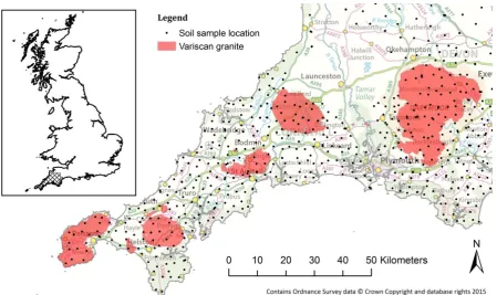
The study area, south west England, is located at the southwestern tip of the British Isles (Fig. 1). A 104
wealth of high resolution geoscientific data has been collected across south west England owing to 105
complex and economically significant geology. In brief summary, the geology of the region consists 106
of a suite of metasedimentary facies originally deposited in a series of Devonian-Carboniferous east-107
west trending basins (Shail and Leveridge, 2009). The granites of the Cornubian Batholith were then 108
emplaced following basin inversion during the late Carboniferous to early Permian Variscan Orogeny 109
(Charoy, 1986; Floyd et al., 1993), and have provided a heat source for extensive hydrothermal 110
activity. The result of this hydrothermal activity is that the region is both rich in polymetallic 111
mineralisation (Dines, 1956; Willis-Richards and Jackson, 1989) and complex in terms of mapping 112
and understanding element distributions (e.g. Colbourn et al., 1975; Alderton et al., 1980; Smedley, 113
1991; Kirkwood et al., 2016). 114
2.2 Target variables - soil geochemical data
115
The soil geochemical data used in this study is derived from samples collected across south west 116
England during the summer field campaign of 2012 by the British Geological Survey following 117
standard Geochemical Baseline Survey of the Environment (G-BASE) methods (Johnson et al., 2005). 118
A total of 568 samples were collected within the study area at an average sampling density of one 119
sample per 12.2 km2 (Fig 1). Samples were collected at random, but exclude coverage of the Tamar 120
Valley area which was sampled in 2004. The Tamar Valley data is not used in this study due to 121
inferior lower limits of detection as a result of advancements in analytical procedure between the 122
years of 2004 and 2012. The soil samples were collected from a depth of 5-20cm and sieved to 123
<2mm grain size before being dried, ground and pelletised prior to analysis by XRF for 48 major and 124
trace elements according to standard G-BASE procedures (Johnson et al., 2005). The 5-20cm 125
sampling depth is intended to target the A horizon of typical soils, with material from the O horizon 126
being excluded with the topmost 5cm. However, soil horizon representation within each sample 127
6 measured. Data quality was assured by the inclusion of duplicate samples, replicate samples, and 129
certified reference materials within the analytical runs. 130
Total concentrations of the following elements were determined along with pH and LOI: Ag, Al, As, 131
Ba, Bi, Br, Ca, Cd, Ce, Co, Cr, Cs, Cu, Fe, Ga, Ge, Hf, I, K, La, Mg, Mn, Mo, Na, Nb, Nd, Ni, P, Pb, Rb, Sb, 132
Sc, Se, Si, Sm, Sn, Sr, Ta, Te, Th, Ti, Tl, U, V, W, Y, Zn and Zr. The major elements (Al, Ca, Fe, K, Mg, 133
Mn, Na, P, Si, Ti, Zr) were assumed to exist as their common oxides, and were each appended with 134
the appropriate additional mass of oxygen so that the sum of all element concentrations for each 135
sample approached 100%, or in the units of the study, 1 million milligrams per kilogram. For most 136
samples though, the chemical analyses do not sum to 100%. This ‘remainder’ (referred to as ‘R’) is 137
included in the study, to see if it too could be modelled and explained. 138
139
[image:6.595.77.527.369.636.2]140
Fig. 1.Locations of 2012 field season G-BASE soil samples within the study area in south west England. The inset map
141
shows the study area (cross-hatched) in reference to the rest of Great Britain. The granites of the Cornubian Batholith are
142
shown as they form prominent geological and geochemical landmarks within the region.
143
2.3 Auxiliary variables – high resolution geophysics and remote sensed data
144
In order to provide the quantile regression forest models with as much information as possible from 145
7 utilised. The available data sets comprise airborne magnetic and radiometric surveys from the Tellus 147
South West project (Beamish et al., 2014), aerial elevation survey from NEXTMap (Intermap 148
Technologies, 2007), land gravity survey from the British Geological Survey et al. (1968), and Landsat 149
8 satellite imagery (Roy et al., 2014). All these auxiliary variables and their derivatives (Table 1) were 150
resampled from their original data grids to a regular 100 m grid covering the study area using 151
bilinear interpolation. 152
The 61,000 line-km of airborne geophysical data collected for the Tellus South West project, and the 153
processing undertaken to produce the original magnetics and radiometrics data grids, is described by 154
Beamish and White (2014). The survey used a N-S line separation of 200 m and a magnetic data 155
sampling of 20 Hz providing a mean along-line sampling of 3.6 m. Radiometric data were sampled at 156
1 Hz intervals providing a sampling of 71 m. Data grids were generated using bicubic spline 157
interpolation (magnetic) and minimum curvature (radiometric). The land gravity survey data were 158
[image:7.595.64.511.458.770.2]gridded using minimum curvature. 159
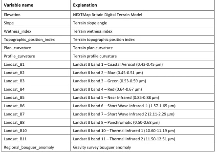
Table 1 160
Explanations of the geophysical and remote sensed variables used in the modelling.
161
Variable name Explanation
Elevation NEXTMap Britain Digital Terrain Model
Slope Terrain slope angle
Wetness_index Terrain wetness index
Topographic_position_index Terrain topographic position index
Plan_curvature Terrain plan curvature
Profile_curvature Terrain profile curvature
Landsat_B1 Landsat 8 band 1 – Coastal Aerosol (0.43-0.45 µm)
Landsat_B2 Landsat 8 band 2 – Blue (0.45-0.51 µm)
Landsat_B3 Landsat 8 band 3 – Green (0.53-0.59 µm)
Landsat_B4 Landsat 8 band 4 – Red (0.64-0.67 µm)
Landsat_B5 Landsat 8 band 5 – Near Infrared (0.85-0.88 µm)
Landsat_B6 Landsat 8 band 6 – Short Wave Infrared 1 (1.57-1.65 µm)
Landsat_B7 Landsat 8 band 7 – Short Wave Infrared 2 (2.11-2.29 µm)
Landsat_B8 Landsat 8 band 8 – Panchromatic (0.50-0.68 µm)
Landsat_B10 Landsat 8 band 10 – Thermal Infrared 1 (10.60-11.19 µm)
Landsat_B11 Landsat 8 band 11 – Thermal Infrared 2 (11.50-12.51 µm)
8
Residual_bouguer_anomaly Gravity survey high pass filtered bouguer anomaly
TMI_IGRF International Geomagnetic Reference Field corrected TMI
TMI_IGRF_1VD 1st vertical derivative of TMI_IGRF
TMI_IGRF_AS Analytical signal of TMI_IGRF
TMI_IGRF_REDP Reduction to the pole of TMI
Radiometrics_uranium Uranium counts from gamma ray spectrometry
Radiometrics_thorium Thorium counts from gamma ray spectrometry
Radiometrics_potassium Potassium counts from gamma ray spectrometry
Radiometrics_total_count Total count of unmixed gamma ray signal
3. Methods
1623.1 Quantile regression forests
163
Quantile regression forests (Meinshausen, 2006) are an elaboration of random forest (Breiman, 164
2001); an ensemble model based on the averaged outputs of multiple decision trees (Breiman et al., 165
1984). Where random forest takes the mean of the outputs of the ensemble of decision trees as the 166
final prediction, quantile regression forests also take specified quantiles from the outputs of the 167
ensemble of decision trees, providing a quantification of the uncertainty associated with each 168
prediction. 169
The decision trees themselves are constructed through recursive partitioning starting with a root 170
node which contains all the data provided to the tree. The root node is split by defining an optimal 171
threshold in whichever auxiliary variable works best to provide two resulting data partitions each 172
with the greatest purity (the least variation in the target variable). This process is then repeated 173
successively on child partitions until the terminal nodes (‘leaves’) are reached, at which point each 174
partition contains just a single sample (or specified small number of samples) whose target variable 175
value (or mean value) is explained by a series of increasingly precise “if-then” conditional statements 176
referring to the context of the sample in the auxiliary variable feature space. 177
If all of the decision trees were grown from the same training data there would be no point in using 178
an ensemble – the trees would all grow identically and the resultant model would be highly liable to 179
9 trees by using bootstrap aggregation, or bagging (Breiman, 1996), to grow each tree from a separate 181
subsample (roughly two thirds) of the full training dataset, thus reducing the chance of fitting to 182
noise when the outputs of the multiple trees are averaged. In addition to bagging, random forest 183
also provides only a random subset of the auxiliary variables on which to make each split in each 184
tree, which reduces the chance of the same very strong predictors being chosen at every split, and 185
therefore prevents trees from becoming overly correlated. The resulting algorithm is recognised as a 186
highly competitive machine learning technique (e.g. Liu et al., 2013; Rodriguez-Galiano et al., 2015). 187
One drawback of the random forest method is that, as a consequence of each prediction being 188
equivalent to a weighted average of the target variable values in the training data set (Lin and Jeon, 189
2006), predictions towards the limits of the training data values are increasingly biased towards the 190
mean. This results in a tendency for low value predictions to exhibit positive bias, and high value 191
predictions to exhibit negative bias (Zhang and Lu, 2012). To correct for this all random forest 192
models were appended with a linear transformation defined by a robust linear model (iterative 193
reweighted least squares; Venables and Ripley, 2013) of observations against random forest 194
predictions during their training phase. This process effectively stretches the predictive range of the 195
random forest in order to correct for central tendency bias. 196
All modelling was conducted in R (R Core Team, 2014) with a framework developed around the 197
randomForest package (Liaw and Wiener, 2002). The models each used 1001 decision trees - a 198
sufficient number to allow convergence of error to a stable minimum. The odd number of trees 199
prevents possible ties in variable importance. Each tree was grown until the terminal nodes 200
contained 8 samples in order to reduce overfitting to outliers. The default number of variables to try 201
at each split – one third of the number of features – was used. The mean of the outputs of the 202
ensemble of decision trees was used as the predicted value, and for each prediction the 2.5th and 203
97.5th percentiles of the ensemble were used as the lower and upper limits of a 95% prediction 204
10
3.2 Model validation
206
The training dataset was constructed by joining the auxiliary variable data at each soil sample site to 207
the geochemical data for each soil sample, using bilinear interpolation, in order to form a single 208
table of both geochemical and auxiliary variable values for each sample site. A stratified 10-fold 209
cross validation process was then used, in which the training data was randomly split into 10 equal 210
folds of approximately equal mean (Kohavi, 1995). Then, for each element, a quantile regression 211
forest model was constructed using the data in 9 of the folds before being tested by predicting the 212
measured element concentrations in the remaining fold. The folds were cycled through and the 213
modelling process repeated so that, in the course of the full 10-fold cross validation, every sample 214
was used as test data. This process allows the accuracy of the model’s predictions and prediction 215
intervals (uncertainty estimates) to be assessed for each element, which is visualised in this study 216
using scatter plots of the predicted against observed values. The prediction interval accuracies are 217
assessed for each model on the basis of how closely the percentage of samples that are observed to 218
fall within the prediction interval match the expected percentage (according to the specified 219
prediction interval). In the case of this study we use a 95% prediction interval and therefore expect 220
that 95% of samples will fall within it during cross-validation. 221
To allow the quality of each element’s model to be compared, cross-validated R2 values, root-mean-222
square error (RMSE) and range-normalised RMSE values were derived according to the relationship 223
between each model’s predictions and the actual measurements. In addition, Moran’s I (Moran, 224
1950) was also calculated on each element’s residuals to provide a measure of residual spatial 225
autocorrelation. The Moran’s I scale runs from -1 (perfect dispersion) to 1 (perfect correlation), with 226
values close to zero indicating spatially random phenomena and suggesting that model performance 227
would not be increased by directly taking spatial autocorrelation into account. 228
In order to provide some context to the prediction accuracy of the quantile regression forest models, 229
11 quantile regression forest modelling during the 10-fold cross validation, from which cross-validated 231
R2 values were derived. 232
3.3 Regional geochemical map production
233
The geochemical maps for each element were produced using a quantile regression forest model 234
constructed on the full 568 sample training dataset. For each element, both concentration and 235
uncertainty maps were produced. The value assigned to each grid cell in the concentration map is a 236
prediction based on the measured values of the auxiliary variables. The value assigned to each grid 237
cell in the uncertainty map is the width of the 95% prediction interval associated with each 238
concentration prediction. No further measurements of soil geochemistry are used to test the map, 239
but the results of the 10-fold cross validation form an acceptable approximation of the performance 240
of each element’s model (and therefore the quality of each element’s map)(Kohavi, 1995; 241
Vanwinckelen and Blockeel, 2012). For further assessment of model quality, the residuals of the 242
quantile regression forests were mapped using inverse distance weighted interpolation. This allows 243
for any spatial patterns within the residuals to be assessed (a more involved alternative to the 244
Moran’s I metric). Concentration maps were also produced by ordinary kriging to allow visual 245
comparison with the quantile regression forest maps. However, caution is advised against making 246
critical comparisons between methods based on the appearance of the maps alone – the image 247
format encourages far more subjective (and potentially misleading) interpretations than objective 248
model quality measures such as cross-validated R2. All maps were symbolised using a CubeHelix 249
continuous colour scale to prevent loss of information when viewing in greyscale (Green, 2011). 250
3.4 Model interpretation
251
With the help of the R package forestFloor (Welling, 2015) partial dependence scatter plots were 252
produced to visualise the contribution of a given variable to the predicted element concentration 253
(Palczewska et al., 2013). Additionally, each quantile regression forest model provides a measure of 254
the average ability of each auxiliary variable to increase node purity in child partitions; thus 255
12 The combination of these outputs provides insight into the controls behind each element’s
257
distribution. 258
4. Results and discussion
2594.1 Model performance
260
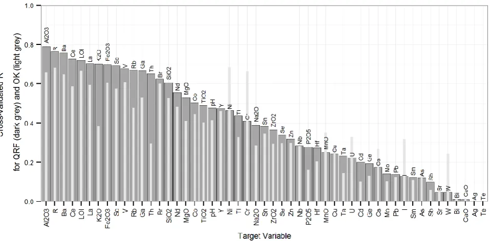
[image:12.595.88.567.218.454.2]261
Fig. 2.Cross-validated R2 values for comparison of quantile regression forest (QRF) model quality between each element
262
(and R, LOI and pH). The corresponding cross-validated R2 values achieved by ordinary kriging (OK) are overlain to provide
263
some context to the overall quality of predictions.
264
Comparison of cross-validated R2 values between quantile regression forests and ordinary kriging 265
reveals that quantile regression forests provide overall improved prediction accuracy for 37 of the 51 266
target variables modelled (Fig. 2). Aside from Ni and Cr, which are unique in the strength of their 267
association with the Lizard Ophiolite Complex (the region's southernmost pensinsula; Kirby, 1979; 268
Kirkwood et al., 2016), the majority of the 14 elements for which ordinary kriging provided better 269
predictions were minor or trace elements, and poorly predicted by either method. This is an 270
encouraging result for the validity of geochemical maps produced by quantile regression forests 271
13 Cross-validated R2 values for the quantile regression forest models vary greatly across the range of 273
elements from 0.79 (Al) to 0 (Te). There appears to be a general inverse relationship between 274
prediction accuracy and element mobility: elements which are known to be relatively immobile (and 275
thus reflect the underlying lithology), such as Al, La and Ce are predicted with little error, while 276
hydrothermally mobile elements such as W,Bi,Te,Ag and As are predicted with higher error. This 277
discrepancy suggests a relative lack of explanation of hydrothermal processes within the suite of 278
auxiliary variables. However, the Moran’s I values for the residuals of all quantile regression forest 279
models (Table 2) only deviate from zero by 0.011 in the worst case (Ge). This suggests that the 280
auxiliary variables used have successfully captured the spatial dependence of all target variables at 281
the scale of the predictor grid. Any residual variation in element concentrations which has not been 282
captured by the models can therefore be attributed to processes which essentially appear to be 283
spatially random at the scale of the geochemical survey, but which additional high resolution 284
auxiliary variables may be capable of explaining. This is supported by inspection of variograms of the 285
residuals of each element (not shown), which appeared to exhibit pure nugget effect. 286
The limited ability of the auxiliary variables used here to explain the distributions of the more mobile 287
elements could perhaps be improved by the inclusion of additional variables which provide more 288
information on spatial context. For example, a measure such as ‘distance to nearest fault’ could 289
provide valuable context in relation to fluid flow pathways. However, a strength of the modelling 290
approach in its current state is the consistency, transparency, and fully quantitative nature of the 291
auxiliary variable datasets; each collected by sensing equipment, thus avoiding the potential 292
inconsistencies of observations made by multiple geologists in the field. Currently any ‘distance to 293
nearest fault’ or similar variables would need to be derived from traditional geological maps and 294
consistency would suffer. However, with sufficient spatial resolution there is no reason why 295
structural features such as faults would not be recognisable within the data. To make the best use of 296
such structural information it would become beneficial to use an approach which is capable of 297
14 properties), perhaps based on artificial neural networks. Such models could potentially learn
299
processes of soil erosion and accumulation (and hydrothermal mobilisation) from spatial context 300
without explicitly being provided with contextual derivatives as input variables. However, such deep 301
learning would increase the effective degrees of freedom within each model, and would require 302
more training data (perhaps more than would ever be financially viable) in order to produce reliable 303
results. The combination of quantile regression forests and the auxiliary variables used in this study 304
therefore represent a promising first step forward given the currently available data and the 305
requirement for transparent and interpretable models. 306
Plots of predicted concentrations against measured concentrations from the 10-fold cross validation 307
of the quantile regression forests allow for more detailed visualisation of model quality. The 308
examples of La and Sn (Fig. 3), chosen as they provide insight into the models of both immobile (La) 309
and mobile (Sn) elements, show how the prediction interval (2.5th to 97.5th forest quantiles) is 310
unique for each prediction. The cross validation has shown these prediction intervals to be a 311
remarkably accurate (if slightly conservative) probabilistic estimate for all elements (see Table. 2). 312
This is very useful; even for elements with relatively low prediction accuracies the prediction 313
intervals still provide reasonable upper and lower limits on predictions, which could be used to drive 314
further geochemical sampling of areas that are of interest as a result of their probable geochemical 315
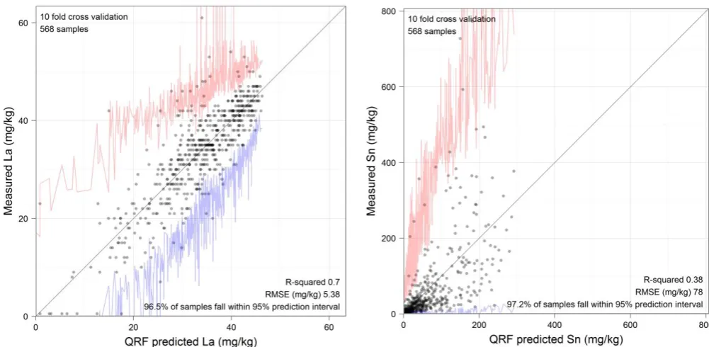
15 317
Fig. 3.Quantile regression forest predicted concentration vs measured concentration scatter plots for La and Sn. For each
318
quantile regression forest prediction the 2.5th percentile is shown in blue and the 97.5th percentile shown in red; these are
319
percentiles of the distribution of the outputs of the individual decision trees in the forest. The range between the 2.5th and
320
97.5th percentiles forms the 95% prediction interval; a measure of the uncertainty associated with each prediction.
321
A comparison of the fit of the predicted values between La and Sn reveals how the fit is deteriorated 322
for the more mobile, highly-skewed, elements; prediction accuracy (and certainty) decreases in the 323
long tail of the data. This is not explicitly due to the data having a skewed distribution, as random 324
forest techniques are scale and transformation invariant. Rather, it is the inevitable result of having 325
fewer data points on which to base the learning of the most ‘extreme’ situations within the context 326
of the auxiliary variables. In this case, these situations are likely to represent relatively rare spikes of 327
localised mineralisation. A geochemical sampling strategy designed around the auxiliary variable 328
feature-space rather than the geographic space would take more samples from the locations of 329
these ‘extreme’ situations and should improve the learning of the distributions of mobile elements 330
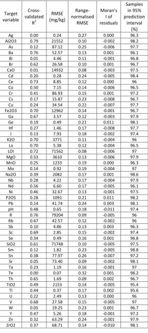
16 Table 2
Cross-validated measures of quantile regression forest model quality.
Target variable Cross-validated R2 RMSE (mg/kg) Range-normalised RMSE Moran's I of residuals Samples in 95% prediction interval (%)
Ag 0.00 0.24 0.27 0.000 96.3
Al2O3 0.79 21552 0.10 -0.002 98.2
As 0.12 87.12 0.25 -0.006 97.7
Ba 0.76 52.57 0.13 0.001 96.1
Bi 0.01 4.46 0.11 -0.001 96.8
Br 0.62 26.58 0.10 0.001 96.7
CaO 0.01 14932 0.08 -0.003 97.5
Cd 0.20 0.28 0.24 -0.005 98.4
Ce 0.73 8.85 0.12 0.000 96
Co 0.50 7.15 0.14 -0.006 96.5
Cr 0.41 86.93 0.15 0.001 97.2
Cs 0.17 15.87 0.23 -0.008 96.7
Cu 0.24 34.54 0.22 -0.007 97.7
Fe2O3 0.70 12962 0.14 -0.001 96.7
Ga 0.67 3.57 0.12 -0.003 97.9
Ge 0.19 0.49 0.21 0.011 98.1
Hf 0.27 1.46 0.17 -0.008 97.7
I 0.13 7.93 0.18 -0.002 97.4
K2O 0.70 3771 0.11 -0.004 96
La 0.70 5.38 0.12 -0.004 96.5
LOI 0.72 71562 0.08 -0.006 97
MgO 0.53 3610 0.13 -0.006 97.9
MnO 0.25 1233 0.19 0.000 96.3
Mo 0.14 0.92 0.19 -0.004 97
Na2O 0.39 2082 0.17 0.001 98.6
Nb 0.28 4.22 0.17 -0.004 97.9
Nd 0.56 6.60 0.17 -0.005 96.1
Ni 0.46 32.67 0.13 -0.001 97.5
P2O5 0.28 1091 0.21 0.011 98.2
Pb 0.14 41.74 0.24 0.003 98.1
pH 0.48 0.65 0.18 -0.011 97.4
R 0.76 79204 0.09 -0.005 96
Rb 0.67 42.57 0.12 -0.002 96
Sb 0.10 4.86 0.13 0.003 96.3
Sc 0.69 2.85 0.15 -0.002 97.4
Se 0.34 0.49 0.16 0.001 96.8
SiO2 0.61 71748 0.10 -0.005 97.5
Sm 0.12 1.82 0.23 -0.005 98.8
Sn 0.38 77.97 0.26 -0.007 97.2
Sr 0.05 73.40 0.09 -0.002 98.1
Ta 0.23 1.19 0.16 -0.001 97
Te 0.00 0.07 0.32 0.001 98.2
Th 0.65 1.69 0.09 0.002 96.7
TiO2 0.49 2153 0.14 -0.005 95.4
Tl 0.44 0.37 0.17 0.002 95.6
U 0.22 2.49 0.13 0.000 96
V 0.68 27.58 0.15 -0.005 97
W 0.05 19.25 0.23 0.001 96.7
Y 0.47 5.26 0.18 -0.001 97.2
Zn 0.32 63.29 0.24 -0.001 97.9
17
4.2 Geochemical maps
332
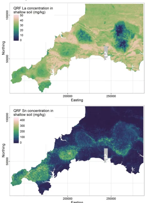
[image:17.595.85.570.76.753.2]333
Fig. 4.Quantile regression forest predicted concentration maps for La and Sn in shallow soils.
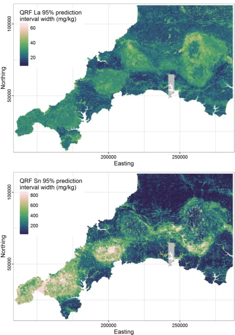
18 335
Fig. 5.Quantile regression forest prediction interval maps for La and Sn in shallow soils.
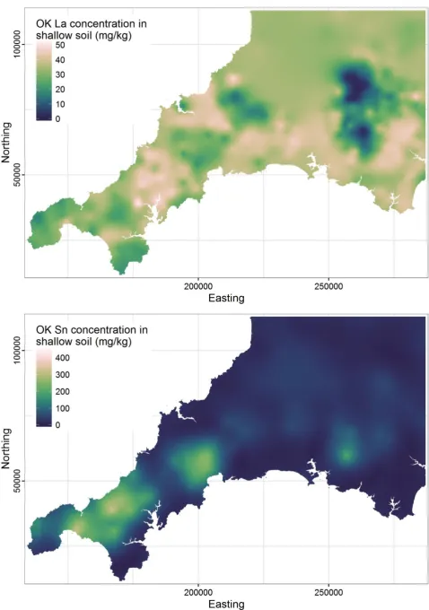
19 337
Fig. 6. Ordinary kriging predicted concentration maps for La and Sn in shallow soils, for comparison.
20 339
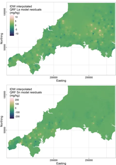
Fig. 7. Quantile regression forest residuals for La and Sn in shallow soils, interpolated using inverse distance weighting.
21 The geochemical maps produced using the quantile regression forest method have a spatial
341
resolution governed by that of the auxiliary variables. Accordingly, with a resolution of 100 m, these 342
maps are capable of resolving the spatial distribution of the elements in much more detail than 343
traditional inverse distance weighted or ordinary kriged interpolated geochemical maps, which are 344
limited by the spatial density of the geochemical sampling. The increased detail is evident when 345
comparing concentration maps produced by quantile regression forests (Fig. 4) and ordinary kriging 346
(Fig. 6). In addition, all quantile regression forest concentration maps are accompanied by 347
uncertainty maps (Fig. 5) in the form of mapped prediction intervals – 95% in the case of this study, 348
but it is possible to map any chosen quantile or interval for each of the quantile regression forest 349
predictions. The quantile regression forest model residual maps (Fig. 7) display the lack of spatial 350
autocorrelation within the residuals in agreement with the Moran’s I results (Table 2). Inverse 351
distance weighted interpolation, rather than kriging, was used to visualise the residuals as their 352
variograms exhibited pure nugget, and kriging would therefore have produced maps of flat zero 353
values. This reinforces the assertion that the quantile regression forest models are accounting for 354
the spatial autocorrelation of the element concentrations at the scale of the auxiliary variable grid. 355
The quantile regression forest maps for both example elements – La and Sn (Fig. 4) provide insight 356
into the geochemistry of the region at a level of detail never before seen. 357
A traditional geochemical map interpretation would involve qualitative comparison of trends seen in 358
the map with trends seen in other datasets. For example, geochemical maps might be compared 359
with geological maps to try to understand the relationships between bedrock geology and surface 360
geochemistry. The details of south west England’s geology are beyond the scope of this paper, but it 361
is well summarised by Shail and Leveridge (2009). A traditional interpretation of the quantile 362
regression forest La map (Fig. 4) might conclude that the concentration of La in soil is strongly 363
constrained by the underlying lithology, a relationship which the high resolution quantile regression 364
forest map reveals in detail. Similarly, a traditional interpretation of the quantile regression forest Sn 365
22 hydrothermal mineralisation and as a result has become concentrated in close proximity to the 367
granite intrusions, though the relationship is not consistent for all intrusions. However, 368
interpretation of the quantile regression forest models themselves, rather than just the geochemical 369
maps, allows the quality of interpretations of the controls on element distributions to be improved 370
over traditional methods. 371
4.2 Controls on element distributions
372
Considering the relative importance of each auxiliary variable to the prediction of each element is a 373
simple means by which to gain insight into the controls on the distributions of each element. In 374
addition to this, partial dependence plots provide insight into the nature of the relationship between 375
each predictor and the target variable. The end user can use this information to devise better 376
informed interpretations and hypotheses of the controls on an element’s distribution. 377
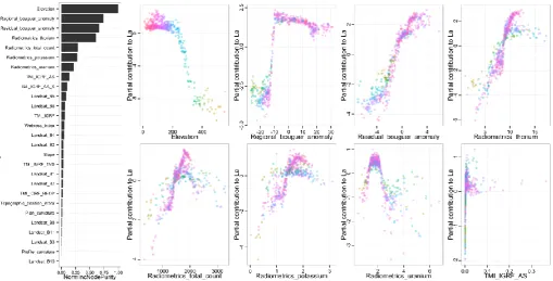
For example, the quantile regression forest model for La concentration finds elevation to be the 378
most important predictor, followed by regional bouguer anomaly, residual bouguer anomaly and 379
radiometric thorium concentration (Fig. 8). The negative correlation between La and elevation at 380
elevations above 200 m indicates a close associated with the granites – which are found outcropping 381
as elevated plateaus at ≤200 m. Furthermore, the association between La and the presence of 382
granites is also evident in the regional bouguer anomaly – whose signal is dominated by the granites 383
– as a sharp transition at around -11 mGal, which represents the granite-country rock contact. As can 384
be expected, the same granite contact is less imposing in the residual bouguer anomaly, which 385
captures fine scale (shallow depth) gravitational variations that are more influenced by other less 386
deep-rooted lithologies in the region. More subtle lithological information in the La map appear to 387
be revealed by the radiometrics data, in particular the relationship between La and Th. The 388
multimodal appearance of this and other partial relationships is an effect of interaction between 389
predictor variables. For example the La–Th relationship appears to fork into two probable trends 390
upwards of 10 ppm of Th. Colouring the points according to elevation reveals that it is an interaction 391
23 upper trend from the lower trend. The lower trend, formed of samples of high elevation and low 393
bouguer anomaly, represents the distinct relationship between La and Th over granites compared to 394
the steeper and more linear relationship between La and Th on the surrounding rocks of lower 395
elevation. 396
In contrast, the quantile regression forest model for Sn concentration finds regional bouguer 397
anomaly, total magnetic intensity (TMI), radiometrics uranium and elevation to be the most 398
important predictors (Fig. 9). The negative correlation between Sn and regional bouguer anomaly 399
can be taken as proxy for the relationship between Sn and granite; generally, Sn values are elevated 400
on and around granite bodies. The gradual transition to the Sn plateau upwards of 10 mGal gives 401
some indication of the mobility of Sn, whose concentrations at the regional scale form gradational 402
rather than sharp boundaries. The relationship between Sn and TMI is complex, but there is a strong 403
negative relationship between Sn concentration and TMI values between -50 and 0 nT, particularly 404
over granite (low regional bouguer anomaly), although it does not extend beyond this range. 405
Similarly, there is a strong positive relationship between Sn and radiometric U between 1.9 and 2.1 406
ppm U which presumably represents the transition onto granite. The broadly negative relationship 407
between Sn and elevation is heavily influenced by interactions. With the help of a regional bouguer 408
anomaly based colour scheme it is apparent that this relationship is relatively weak over the 409
granites, but indicates increased Sn concentrations at lower granite elevations. This may represent 410
the fact that, on average, the interiors of the granites have lower Sn concentrations than the 411
perimeters due to differentiation between granite phases, and the influence of hydrothermal 412
processes. The off-granite relationship is stronger, and shows an almost exponential increase in Sn 413
concentrations descending towards sea level from an elevation of about 100 m, above which the 414
influence of elevation on Sn is fairly negligible. This may relate to Sn enrichment of floodplains as a 415
result of sediment transport from mineralised areas. 416
24
4.3 A note on compositions, LOI and the unmeasured ‘remainder’, R.
418
Despite not implementing compositional data analysis methods (Aitchison, 1986; Egozcue et al., 419
2003; Pawlowsky-Glahn and Buccianti, 2011) to intrinsically ensure that modelled element 420
concentrations sum to 100% at every prediction point (at the cost of computational expense and 421
additional complexity to interpretations), we find that the sum of predicted concentrations of 422
measured elements, and the unmeasured ‘remainder’ (R), fall very close to 100% in the vast majority 423
of situations (Fig. 10). The 95% interval of summed predictions (predicted element concentrations 424
plus predicted remainder concentration) spans from 96.0% to 105.4%. In addition, we find that R has 425
a very close relationship with loss on ignition (LOI): their quadratic relationship could be explained 426
by a discrepancy in calibration between the two measurement methods, but it appears that they are 427
essentially two separate measures of the same thing (Fig. 11). The models of LOI and R achieved 428
some of the highest prediction accuracies in the study according to the cross-validated R2 and 429
normalised RMSE metrics (Table 2). 430
431
[image:24.595.77.587.438.697.2]432
Fig. 8.Variable importance plot and top eight most important partial dependence plots for La, with points
433
coloured according to elevation (the most important predictor).
25 435
Fig. 9.Variable importance plot and top eight most important partial dependence plots for Sn, with points
436
coloured according to regional bouguer anomaly (the most important predictor).
437
438
Fig. 10.Sum of predicted element concentrations + R.
[image:25.595.81.325.360.606.2]26 440
Fig. 11. Relationship between LOI and R in training data. The equation describes a quadratic curve (red line) which fits the
441
data with an R2 of 0.98.
442
5. Conclusions
443The implementation of quantile regression forests to map regional soil geochemistry at high 444
resolution (100 m) using only information from auxiliary variables has produced very encouraging 445
results. The major, immobile, elements are modelled with sufficient accuracy to promote the 446
development of fully quantitative geological mapping using remotely sensed data such as those used 447
in this study. Immobile elements are modelled with a lesser degree of accuracy due to a combination 448
of the relative under-sampling of their ‘extreme’ events (which could be improved with a change in 449
sampling design to target anomalous locations in the context of the available auxiliary variables) and 450
perhaps a lack of relevant information in existing auxiliary variables. Further developments to 451
sampling design strategies, sensing technologies, and auxiliary variable derivatives (or the use of 452
more advanced learners) should be capable of improving the modelling of mobile elements in the 453
future. 454
For now, these models are capable of making an interpretable and uncertainty-aware prediction of 455
27 spectral and topographic information. The prediction process is similar to the decision making 457
process which might be made by a human, but with the objectivity and accuracy of an optimally self-458
training algorithm. Allowing the model to consider the spatial dependence of the target variables 459
might gain improvements in some situations, but the Moran’s I results of the residuals suggest that 460
the processes controlling the residuals appear to be operating randomly at the scale of the 461
geochemical survey, and so it is the case that we currently do not have sufficient information to 462
explain them. 463
The maps produced by the quantile regression forests are more useful than their spatially 464
interpolated equivalents, providing increased detail, accuracy, interpretability and uncertainty 465
awareness. Accordingly, the use of machine learning methods in conjunction with geophysical, 466
radiometric, spectral and topographic information seems very capable of bringing significant 467
improvements to geological mapping, agriculture, environmental survey and mineral exploration 468
practices, and all the policies that surround them. 469
Acknowledgements
470This research was funded by the British Geological Survey. Thanks to all colleagues and reviewers 471
who have helped to guide this study. Thanks also to all G-BASE volunteers for their hard work in 472
collecting a valuable geochemical dataset. 473
Aitchison, J., 1986. The statistical analysis of compositional data. Chapman & Hall, London. 474
Alderton, D., Pearce, J.A., Potts, P., 1980. Rare earth element mobility during granite alteration: 475
evidence from southwest England. Earth and Planetary Science Letters 49, 149-165. 476
Alloway, B.J., 1990. Heavy metals in soils. Blackie & Son Ltd. 477
Appleton, J., Ridgway, J., 1993. Regional geochemical mapping in developing countries and its 478
application to environmental studies. Applied geochemistry 8, 103-110. 479
Beamish, D., Howard, A.S., Ward, E.K., White, J., Young, M.E., 2014. Tellus South West airborne 480
geophysical data. Natural Environment Research Council, British Geological Survey. 481
Beus, A.A., Grigorian, S.V., 1977. Geochemical exploration methods for mineral deposits. 482
Bowie, S.H.U., Thornton, I., 1985. Environmental geochemistry and health. Springer Science & 483
Business Media. 484
Breiman, L., 1996. Bagging predictors. Machine learning 24, 123-140. 485
Breiman, L., 2001. Random forests. Machine learning 45, 5-32. 486
Breiman, L., Friedman, J., Stone, C.J., Olshen, R.A., 1984. Classification and regression trees. CRC 487
28 British Geological Survey et al., 1968. GB Land Gravity Survey. British Geological Survey.
489
Carranza, E.J.M., Laborte, A.G., 2015. Random forest predictive modeling of mineral prospectivity 490
with small number of prospects and data with missing values in Abra (Philippines). 491
Computers & Geosciences 74, 60-70. 492
Colbourn, P., Alloway, B., Thornton, I., 1975. Arsenic and heavy metals in soils associated with 493
regional geochemical anomalies in south-west England. Science of the Total Environment 4, 494
359-363. 495
Cracknell, M.J., Reading, A.M., 2014. Geological mapping using remote sensing data: A comparison 496
of five machine learning algorithms, their response to variations in the spatial distribution of 497
training data and the use of explicit spatial information. Computers & Geosciences 63, 22-33. 498
Cressie, N., 1988. Spatial prediction and ordinary kriging. Mathematical Geology 20, 405-421. 499
Cutler, D.R., Edwards Jr, T.C., Beard, K.H., Cutler, A., Hess, K.T., Gibson, J., Lawler, J.J., 2007. Random 500
forests for classification in ecology. Ecology 88, 2783-2792. 501
Darnley, A.G., 1990. International geochemical mapping: a new global project. Journal of 502
Geochemical Exploration 39, 1-13. 503
Dines, H.G., 1956. The metalliferous mining region of south-west England. HM Stationery Office. 504
Egozcue, J.J., Pawlowsky-Glahn, V., Mateu-Figueras, G., Barcelo-Vidal, C., 2003. Isometric logratio 505
transformations for compositional data analysis. Mathematical Geology 35, 279-300. 506
Evans, J.S., Murphy, M.A., Holden, Z.A., Cushman, S.A., 2011. Modeling species distribution and 507
change using random forest, Predictive Species and Habitat Modeling in Landscape Ecology. 508
Springer, pp. 139-159. 509
Fordyce, F.M., 2013. Selenium deficiency and toxicity in the environment. Springer. 510
Gislason, P.O., Benediktsson, J.A., Sveinsson, J.R., 2006. Random forests for land cover classification. 511
Pattern Recognition Letters 27, 294-300. 512
Green, D., 2011. A colour scheme for the display of astronomical intensity images. arXiv preprint 513
arXiv:1108.5083. 514
Harris, J., Grunsky, E., Behnia, P., Corrigan, D., 2015. Data-and knowledge-driven mineral 515
prospectivity maps for Canada's North. Ore Geology Reviews. 516
Hawkes, H.E., Webb, J.S., 1962. Geochemistry in mineral exploration. 517
Henderson, B.L., Bui, E.N., Moran, C.J., Simon, D., 2005. Australia-wide predictions of soil properties 518
using decision trees. Geoderma 124, 383-398. 519
Hengl, T., Heuvelink, G.B., Stein, A., 2003. Comparison of kriging with external drift and regression-520
kriging. Technical note, ITC 51. 521
Hiemstra, P.H., Pebesma, E.J., Twenhöfel, C.J., Heuvelink, G.B., 2009. Real-time automatic 522
interpolation of ambient gamma dose rates from the Dutch radioactivity monitoring 523
network. Computers & Geosciences 35, 1711-1721. 524
Intermap Technologies, 2007. NEXTMap British Digital Terrain Model Dataset Produced by Intermap, 525
NERC Earth Observation Data Centre. 526
Johnson, C., Breward, N., Ander, E., Ault, L., 2005. G-BASE: baseline geochemical mapping of Great 527
Britain and Northern Ireland. Geochemistry: Exploration, Environment, Analysis 5, 347-357. 528
Jordan, W.J., Alloway, B.J., Thornton, I., 1975. The application of regional geochemical 529
reconnaissance data in areas of arable cropping. Journal of the Science of Food and 530
Agriculture 26, 1413-1423. 531
Kirby, G., 1979. The Lizard complex as an ophiolite. 532
Kirkwood, C., Everett, P., Ferreira, A., Lister, B., 2016. Stream sediment geochemistry as a tool for 533
enhancing geological understanding: An overview of new data from south west England. 534
Journal of Geochemical Exploration 163, 28-40. 535
Knotters, M., Brus, D., Voshaar, J.O., 1995. A comparison of kriging, co-kriging and kriging combined 536
with regression for spatial interpolation of horizon depth with censored observations. 537
Geoderma 67, 227-246. 538
Kohavi, R., 1995. A study of cross-validation and bootstrap for accuracy estimation and model 539
29 Lawrence, R.L., Wood, S.D., Sheley, R.L., 2006. Mapping invasive plants using hyperspectral imagery 541
and Breiman Cutler classifications (RandomForest). Remote Sensing of Environment 100, 542
356-362. 543
Levinson, A.A., 1974. Introduction to exploration geochemistry.[Textbook]. 544
Lewis, G., Thornton, I., Howarth, R., 1986. Geochemistry and animal health, Applied geochemistry in 545
the 1980s: proceedings of a meeting to honour the contribution of professor John S. Webb 546
to applied geochemistry, held on 29 April 1983 at Imperial College, London. John Wiley & 547
Sons, p. 260. 548
Liaw, A., Wiener, M., 2002. Classification and regression by randomforest. R News 2 (3): 18–22. URL: 549
http://CRAN.R-project.org/doc/Rnews.
550
Lin, Y., Jeon, Y., 2006. Random forests and adaptive nearest neighbors. Journal of the American 551
Statistical Association 101, 578-590. 552
Liu, M., Wang, M., Wang, J., Li, D., 2013. Comparison of random forest, support vector machine and 553
back propagation neural network for electronic tongue data classification: Application to the 554
recognition of orange beverage and Chinese vinegar. Sensors and Actuators B: Chemical 177, 555
970-980. 556
Meinshausen, N., 2006. Quantile regression forests. The Journal of Machine Learning Research 7, 557
983-999. 558
Moran, P.A., 1950. Notes on continuous stochastic phenomena. Biometrika, 17-23. 559
Palczewska, A., Palczewski, J., Robinson, R.M., Neagu, D., 2013. Interpreting random forest models 560
using a feature contribution method, Information Reuse and Integration (IRI), 2013 IEEE 14th 561
International Conference on. IEEE, pp. 112-119. 562
Pawlowsky-Glahn, V., Buccianti, A., 2011. Compositional data analysis: Theory and applications. John 563
Wiley & Sons. 564
R Core Team, 2014. R: A Language and Environment for Statistical Computing, R version 3.1.1 (2014-565
07-10) ed. R Foundation for Statistical Computing, Vienna, Austria. 566
Reid, R., Horvath, D., 1980. Soil chemistry and mineral problems in farm livestock. A review. Animal 567
Feed Science and Technology 5, 95-167. 568
Reimann, C., Siewers, U., Tarvainen, T., Bityukova, L., Eriksson, J., Gilucis, A., Gregorauskiene, V., 569
Lukashev, V., Matinian, N., Pasieczna, A., 2003. Agricultural soils in Northern Europe: a 570
geochemical atlas. E. Schweizerbart'sche Verlagsbuchhandlung. 571
Rodriguez-Galiano, V., Sanchez-Castillo, M., Chica-Olmo, M., Chica-Rivas, M., 2015. Machine learning 572
predictive models for mineral prospectivity: An evaluation of neural networks, random 573
forest, regression trees and support vector machines. Ore Geology Reviews. 574
Rodriguez-Galiano, V.F., Ghimire, B., Rogan, J., Chica-Olmo, M., Rigol-Sanchez, J.P., 2012. An 575
assessment of the effectiveness of a random forest classifier for land-cover classification. 576
ISPRS Journal of Photogrammetry and Remote Sensing 67, 93-104. 577
Roy, D.P., Wulder, M., Loveland, T., Woodcock, C., Allen, R., Anderson, M., Helder, D., Irons, J., 578
Johnson, D., Kennedy, R., 2014. Landsat-8: Science and product vision for terrestrial global 579
change research. Remote Sensing of Environment 145, 154-172. 580
Salminen, R., Tarvainen, T., Demetriades, A., Duris, M., Fordyce, F., Gregorauskiene, V., Kahelin, H., 581
Kivisilla, J., Klaver, G., Klein, H., 1998. FOREGS geochemical mapping field manual. 582
Shail, R.K., Leveridge, B.E., 2009. The Rhenohercynian passive margin of SW England: Development, 583
inversion and extensional reactivation. Comptes Rendus Geoscience 341, 140-155. 584
Smedley, P.L., 1991. The geochemistry of rare earth elements in groundwater from the Carnmenellis 585
area, southwest England. Geochimica et Cosmochimica Acta 55, 2767-2779. 586
Thornton, I., 1993. Environmental geochemistry and health in the 1990s: a global perspective. 587
Applied geochemistry 8, 203-210. 588
Thornton, I., Plant, J., 1980. Regional geochemical mapping and health in the United Kingdom. 589
Journal of the Geological Society 137, 575-586. 590
Vanwinckelen, G., Blockeel, H., 2012. On estimating model accuracy with repeated cross-validation, 591
BeneLearn 2012: Proceedings of the 21st Belgian-Dutch Conference on Machine Learning, 592
30 Venables, W.N., Ripley, B.D., 2013. Modern applied statistics with S-PLUS. Springer Science &
594
Business Media. 595
Webb, J., Thornton, I., Nichol, I., 1971. The agricultural significance of regional geochemical 596
reconnaissance in the United Kingdom. Trace Elements in Soils and Crops, Min. Agr. Fish. 597
Food Tech. Bull 21, 1-7. 598
Welling, S.H., 2015. forestFloor: Visualizes Random Forests with Feature Contributions. URL: 599
http://CRAN.R-project.org/package=forestFloor.
600
White, J.G., Zasoski, R.J., 1999. Mapping soil micronutrients. Field Crops Research 60, 11-26. 601
Wiesmeier, M., Barthold, F., Blank, B., Kögel-Knabner, I., 2011. Digital mapping of soil organic matter 602
stocks using Random Forest modeling in a semi-arid steppe ecosystem. Plant and soil 340, 7-603
24. 604
Willis-Richards, J., Jackson, N.J., 1989. Evolution of the Cornubian ore field, Southwest England; Part 605
I, Batholith modeling and ore distribution. Economic Geology 84, 1078-1100. 606
Xu, Y., Cheng, Q., 2001. A fractal filtering technique for processing regional geochemical maps for 607
mineral exploration. Geochemistry: Exploration, environment, analysis 1, 147-156. 608
Xuejing, X., Xueqiu, W., 1991. Geochemical exploration for gold: a new approach to an old problem. 609
Journal of Geochemical Exploration 40, 25-48. 610
Zhang, G., Lu, Y., 2012. Bias-corrected random forests in regression. Journal of Applied Statistics 39, 611
151-160. 612