ISP: Learning Inferential Selectional Preferences

ISP: Learning Inferential Selectional Preferences

Patrick Pantel

†

, Rahul Bhagat

†

,

Bonaventura Coppola

‡

,

Timothy Chklovski

†,

Eduard Hovy

†

†

Information Sciences Institute

University of Southern California

Marina del Rey, CA

{pantel,rahul,timc,hovy}@isi.edu

‡

ITC-Irst and University of Trento

Via Sommarive, 18 – Povo 38050

Trento, Italy

[email protected]

Abstract

Semantic inference is a key component for advanced natural language under-standing. However, existing collections of automatically acquired inference rules have shown disappointing results when used in applications such as textual en-tailment and question answering. This

pa-per presents ISP, a collection of methods

for automatically learning admissible ar-gument values to which an inference rule

can be applied, which we call inferential

selectional preferences, and methods for filtering out incorrect inferences. We

evaluate ISP and present empirical

evi-dence of its effectiveness.

1

Introduction

Semantic inference is a key component for ad-vanced natural language understanding. Several important applications are already relying heavily on inference, including question answering (Moldovan et al. 2003; Harabagiu and Hickl 2006), information extraction (Romano et al. 2006), and textual entailment (Szpektor et al. 2004).

In response, several researchers have created re-sources for enabling semantic inference. Among manual resources used for this task are WordNet (Fellbaum 1998) and Cyc (Lenat 1995). Although important and useful, these resources primarily

contain prescriptive inference rules such as “X

di-vorces Y ⇒X married Y”. In practical NLP

appli-cations, however, plausible inference rules such as

“X married Y” ⇒ “X dated Y” are very useful. This,

along with the difficulty and labor-intensiveness of generating exhaustive lists of rules, has led

re-searchers to focus on automatic methods for build-ing inference resources such as inference rule collections (Lin and Pantel 2001; Szpektor et al. 2004) and paraphrase collections (Barzilay and McKeown 2001).

Using these resources in applications has been hindered by the large amount of incorrect infer-ences they generate, either because of altogether incorrect rules or because of blind application of plausible rules without considering the context of the relations or the senses of the words. For exam-ple, consider the following sentence:

Terry Nichols was charged by federal prosecutors for murder and conspiracy in the Oklahoma City bombing.

and an inference rule such as:

X is charged by Y ⇒ Y announced the arrest of X (1)

Using this rule, we can infer that “federal

prosecu-tors announced the arrest of Terry Nichols”. How-ever, given the sentence:

Fraud was suspected when accounts were charged by CCM telemarketers without obtaining consumer authorization.

the plausible inference rule (1) would incorrectly

infer that “CCM telemarketers announced the

ar-rest of accounts”.

This example depicts a major obstacle to the ef-fective use of automatically learned inference rules. What is missing is knowledge about the ad-missible argument values for which an inference

rule holds, which we call Inferential Selectional

Preferences. For example, inference rule (1)

should only be applied if X is a Person and Y is a

Law Enforcement Agent or a Law Enforcement Agency. This knowledge does not guarantee that the inference rule will hold, but, as we show in this paper, goes a long way toward filtering out errone-ous applications of rules.

In this paper, we propose ISP, a collection of

methods for learning inferential selectional prefer-ences and filtering out incorrect inferprefer-ences. The

presented algorithms apply to any collection of inference rules between binary semantic relations,

such as example (1). ISP derives inferential

selec-tional preferences by aggregating statistics of in-ference rule instantiations over a large corpus of

text. Within ISP, we explore different probabilistic

models of selectional preference to accept or reject specific inferences. We present empirical evidence to support the following main contribution:

Claim: Inferential selectional preferences can be

automatically learned and used for effectively fil-tering out incorrect inferences.

2

Previous Work

Selectional preference (SP) as a foundation for computational semantics is one of the earliest top-ics in AI and NLP, and has its roots in (Katz and Fodor 1963). Overviews of NLP research on this theme are (Wilks and Fass 1992), which includes the influential theory of Preference Semantics by Wilks, and more recently (Light and Greiff 2002).

Rather than venture into learning inferential SPs, much previous work has focused on learning SPs for simpler structures. Resnik (1996), the seminal paper on this topic, introduced a statistical model for learning SPs for predicates using an un-supervised method.

Learning SPs often relies on an underlying set of

semantic classes, as in both Resnik’s and our ap-proach. Semantic classes can be specified manu-ally or derived automaticmanu-ally. Manual collections of semantic classes include the hierarchies of WordNet (Fellbaum 1998), Levin verb classes (Levin 1993), and FrameNet (Baker et al. 1998). Automatic derivation of semantic classes can take a variety of approaches, but often uses corpus methods and the Distributional Hypothesis (Harris 1964) to automatically cluster similar entities into classes, e.g. CBC (Pantel and Lin 2002). In this paper, we experiment with two sets of semantic classes, one from WordNet and one from CBC.

Another thread related to our work includes ex-tracting from text corpora paraphrases (Barzilay and McKeown 2001) and inference rules, e.g.

TEASE1 (Szpektor et al. 2004) and DIRT (Lin and

Pantel 2001). While these systems differ in their approaches, neither provides for the extracted

1

Some systems refer to inferences they extract as entail-ments; the two terms are sometimes used interchangeably.

ference rules to hold or fail based on SPs. Zanzotto et al. (2006) recently explored a different interplay between SPs and inferences. Rather than examine the role of SPs in inferences, they use SPs of a

par-ticular type to derive inferences. For instance the

preference of win for the subject player, a

nomi-nalization of play, is used to derive that “win ⇒

play”. Our work can be viewed as complementary to the work on extracting semantic inferences and paraphrases, since we seek to refine when a given inference applies, filtering out incorrect inferences.

3

Selectional Preference Models

The aim of this paper is to learn inferential selec-tional preferences for filtering inference rules.

Let pi⇒pj be an inference rule where p is a

bi-nary semantic relation between two entities x and

y. Let 〈x, p, y〉 be an instance of relation p.

Formal task definition: Given an inference rule

pi ⇒ pj and the instance 〈x, pi, y〉, our task is to determine if 〈x, pj, y〉 is valid.

Consider the example in Section 1 where we

have the inference rule “X is charged by Y” ⇒ “Y

announced the arrest of X”. Our task is to

auto-matically determine that “federal prosecutors

an-nounced the arrest of Terry Nichols” (i.e.,

〈Terry Nichols, pj, federal prosecutors〉) is valid

but that “CCM telemarketers announced the arrest

of accounts” is invalid.

Because the semantic relations p are binary, the

selectional preferences on their two arguments may be either considered jointly or independently. For

example, the relation p = “X is charged by Y”

could have joint SPs:

〈Person, Law Enforcement Agent〉

〈Person, Law Enforcement Agency〉 (2) 〈Bank Account, Organization〉

or independent SPs:

〈Person, *〉

〈*, Organization〉 (3) 〈*, Law Enforcement Agent〉

This distinction between joint and independent selectional preferences constitutes the difference between the two models we present in this section.

The remainder of this section describes the ISP

selectional preference models. Finally, we propose inference filtering algorithms in Section 3.3.

3.1 Relational Selectional Preferences

Resnik (1996) defined the selectional preferences of a predicate as the semantic classes of the words that appear as its arguments. Similarly, we define the relational selectional preferences of a binary

semantic relation pi as the semantic classes C(x) of

the words that can be instantiated for x and as the

semantic classes C(y) of the words that can be

in-stantiated for y.

The semantic classes C(x) and C(y) can be

ob-tained from a conceptual taxonomy as proposed in (Resnik 1996), such as WordNet, or from the classes extracted from a word clustering algorithm such as CBC (Pantel and Lin 2002). For example,

given the relation “X is charged by Y”, its

rela-tional selection preferences from WordNet could be {social_group, organism, state…} for X and {authority, state, section…}for Y.

Below we propose joint and independent mod-els, based on a corpus analysis, for automatically determining relational selectional preferences.

Model 1: Joint Relational Model (JRM)

Our joint model uses a corpus analysis to learn SPs for binary semantic relations by considering their arguments jointly, as in example (2).

Given a large corpus of English text, we first

find the occurrences of each semantic relation p.

For each instance 〈x, p, y〉, we retrieve the sets C(x)

and C(y) of the semantic classes that x and y

be-long to and accumulate the frequencies of the

tri-ples 〈c(x), p, c(y)〉, where c(x) ∈ C(x) and

c(y) ∈C(y)2.

Each triple 〈c(x), p, c(y)〉 is a candidate

selec-tional preference for p. Candidates can be incorrect

when: a) they were generated from the incorrect

sense of a polysemous word; or b) p does not hold

for the other words in the semantic class.

Intuitively, we have more confidence in a par-ticular candidate if its semantic classes are closely

associated given the relation p. Pointwise mutual

information (Cover and Thomas 1991) is a com-monly used metric for measuring this association

strength between two events e1 and e2:

2

In this paper, the semantic classes C(x) and C(y) are ex-tracted from WordNet and CBC (described in Section 4.2).

( )

( ) ( )1 2 2 1 2 1 , log ) ; ( e P e P e e P e e

pmi = (3.1)

We define our ranking function as the strength

of association between two semantic classes, cx and

cy 3

, given the relation p:

(

)

_{( )}

(

_{( )}

)

p c P p c P p c c P p c p c pmi y x y x y x , log

; = (3.2)

Let |cx, p, cy| denote the frequency of observing

the instance 〈c(x), p, c(y)〉. We estimate the

prob-abilities of Equation 3.2 using maximum likeli-hood estimates over our corpus:

( ) _{∗ ∗}∗ = , , , , p p c p c P x

x

( )

_{∗ ∗}

∗ = , , , , p c p p c

P y y

(

)

∗ ∗ = , , , , , p c p c p c c

P x y x y

(3.3)

Similarly to (Resnik 1996), we estimate the above frequencies using:

( ) ∑ ∈ ∗ = ∗ x c w x w C p w p

c, , , ,

( ) ∑ ∈ ∗ = ∗ y c w y w C w p c

p, , ,

, ∑ _{( ) ( )}

∈

∈ ×

=

y xw c

c w y x w C w C w p w c p c 2

1 , 1 2

2 1, , ,

,

where |x, p, y| denotes the frequency of observing

the instance 〈x, p, y〉 and |C(w)| denotes the number

of classes to which word w belongs. |C(w)|

distrib-utes w’s mass equally to all of its senses cw.

Model 2: Independent Relational Model (IRM)

Because of sparse data, our joint model can miss some correct selectional preference pairs. For ex-ample, given the relation

Y announced the arrest of X

we may find occurrences from our corpus of the

particular class “Money Handler” for X and “

Law-yer” for Y, however we may never see both of

these classes co-occurring even though they would form a valid relational selectional preference.

To alleviate this problem, we propose a second model that is less strict by considering the argu-ments of the binary semantic relations independ-ently, as in example (3).

Similarly to JRM, we extract each instance

〈x, p, y〉 of each semantic relation p and retrieve the

set of semantic classes C(x) and C(y) that x and y

belong to, accumulating the frequencies of the

tri-ples 〈c(x), p, *〉 and 〈*, p, c(y)〉, where

c(x) ∈C(x) and c(y) ∈C(y).

All tuples 〈c(x), p, *〉 and 〈*, p, c(y)〉 are

candi-date selectional preferences for p. We rank

candi-dates by the probability of the semantic class given

the relation p, according to Equations 3.3.

3

3.2 Inferential Selectional Preferences

Whereas in Section 3.1 we learned selectional

preferences for the arguments of a relation p, in

this section we learn selectional preferences for the

arguments of an inference rule pi⇒pj.

Model 1: Joint Inferential Model (JIM)

Given an inference rule pi ⇒ pj, our joint model

defines the set of inferential SPs as the intersection

of the relational SPs for pi and pj, as defined in the

Joint Relational Model (JRM). For example,

sup-pose relation pi = “X is charged by Y” gives the

following SP scores under the JRM:

〈Person, pi, Law Enforcement Agent〉 = 1.45 〈Person, pi, Law Enforcement Agency〉 = 1.21

〈Bank Account, pi, Organization〉 = 0.97

and that pj = “Y announced the arrest of X” gives

the following SP scores under the JRM:

〈Law Enforcement Agent, pj, Person〉 = 2.01 〈Reporter, pj, Person〉 = 1.98 〈Law Enforcement Agency, pj, Person〉 = 1.61

The intersection of the two sets of SPs forms the

candidate inferential SPs for the inference pi⇒pj:

〈Law Enforcement Agent, Person〉 〈Law Enforcement Agency, Person〉

We rank the candidate inferential SPs according to three ways to combine their relational SP scores,

using the minimum, maximum, and average of the

SPs. For example, for 〈Law Enforcement Agent,

Person〉, the respective scores would be 1.45, 2.01, and 1.73. These different ranking strategies pro-duced nearly identical results in our experiments, as discussed in Section 5.

Model 2: Independent Inferential Model (IIM)

Our independent model is the same as the joint model above except that it computes candidate in-ferential SPs using the Independent Relational Model (IRM) instead of the JRM. Consider the

same example relations pi and pj from the joint

model and suppose that the IRM gives the

follow-ing relational SP scores for pi:

〈Law Enforcement Agent, pi, *〉 = 3.43 〈*, pi, Person〉 = 2.17 〈*, pi, Organization〉 = 1.24

and the following relational SP scores for pj:

〈*, pj, Person〉 = 2.87 〈Law Enforcement Agent, pj, *〉 = 1.92

〈Reporter, pj, *〉 = 0.89

The intersection of the two sets of SPs forms the

candidate inferential SPs for the inference pi⇒pj:

〈Law Enforcement Agent, *〉 〈*, Person〉

We use the same minimum, maximum, and

av-erage ranking strategies as in JIM.

3.3 Filtering Inferences

Given an inference rule pi ⇒ pj and the instance

〈x, pi, y〉, the system’s task is to determine whether

〈x, pj, y〉 is valid. Let C(w) be the set of semantic

classes c(w) to which word w belongs. Below we

present three filtering algorithms which range from the least to the most permissive:

•ISP.JIM, accepts the inference 〈x, pj, y〉 if the

inferential SP 〈c(x), pj, c(y)〉 was admitted by the

Joint Inferential Model for some c(x) ∈C(x) and

c(y) ∈C(y).

•ISP.IIM.∧, accepts the inference 〈x, pj, y〉 if the

inferential SPs 〈c(x), pj, *〉 AND 〈*, pj, c(y)〉 were

admitted by the Independent Inferential Model for some c(x) ∈C(x) and c(y) ∈C(y) .

•ISP.IIM.∨, accepts the inference 〈x, pj, y〉 if the

inferential SP 〈c(x), pj, *〉 OR 〈*, pj, c(y)〉 was

admitted by the Independent Inferential Model for some c(x) ∈C(x) and c(y) ∈C(y) .

Since both JIM and IIM use a ranking score in their inferential SPs, each filtering algorithm can be tuned to be more or less strict by setting an ac-ceptance threshold on the ranking scores or by

se-lecting only the top τ percent highest ranking SPs.

In our experiments, reported in Section 5, we

tested each model using various values of τ.

4

Experimental Methodology

This section describes the methodology for testing our claim that inferential selectional preferences can be learned to filter incorrect inferences.

Given a collection of inference rules of the form

pi⇒pj, our task is to determine whether a

particu-lar instance 〈x, pj, y〉 holds given that 〈x, pi, y〉

holds4. In the next sections, we describe our

collec-tion of inference rules, the semantic classes used for forming selectional preferences, and evaluation criteria for measuring the filtering quality.

4 _{Recall that the inference rules we consider in this paper are}

4.1 Inference Rules

Our models for learning inferential selectional preferences can be applied to any collection of in-ference rules between binary semantic relations. In this paper, we focus on the inference rules con-tained in the DIRT resource (Lin and Pantel 2001). DIRT consists of over 12 million rules which were extracted from a 1GB newspaper corpus (San Jose Mercury, Wall Street Journal and AP Newswire from the TREC-9 collection). For example, here

are DIRT’s top 3 inference rules for “X solves Y”:

“Y is solved by X”, “X resolves Y”, “X finds a solution to Y”

4.2 Semantic Classes

The choice of semantic classes is of great impor-tance for selectional preference. One important aspect is the granularity of the classes. Too general a class will provide no discriminatory power while too fine-grained a class will offer little generaliza-tion and apply in only extremely few cases.

The absence of an attested high-quality set of semantic classes for this task makes discovering preferences difficult. Since many of the criteria for developing such a set are not even known, we de-cided to experiment with two very different sets of semantic classes, in the hope that in addition to learning semantic preferences, we might also un-cover some clues for the eventual decisions about what makes good semantic classes in general.

Our first set of semantic classes was directly ex-tracted from the output of the CBC clustering algo-rithm (Pantel and Lin 2002). We applied CBC to the TREC-9 and TREC-2002 (Aquaint) newswire collections consisting of over 600 million words. CBC generated 1628 noun concepts and these were used as our semantic classes for SPs.

Secondly, we extracted semantic classes from WordNet 2.1 (Fellbaum 1998). In the absence of any externally motivated distinguishing features (for example, the Basic Level categories from Pro-totype Theory, developed by Eleanor Rosch (1978)), we used the simple but effective method

of manually truncating the noun synset hierarchy5

and considering all synsets below each cut point as part of the semantic class at that node. To select the cut points, we inspected several different hier-archy levels and found the synsets at a depth of 4

5

Only nouns are considered since DIRT semantic relations connect only nouns.

to form the most natural semantic classes. Since the noun hierarchy in WordNet has an average depth of 12, our truncation created a set of con-cepts considerably coarser-grained than WordNet itself. The cut produced 1287 semantic classes, a number similar to the classes in CBC. To properly test WordNet as a source of semantic classes for our selectional preferences, we would need to ex-periment with different extraction algorithms.

4.3 Evaluation Criteria

The goal of the filtering task is to minimize false positives (incorrectly accepted inferences) and false negatives (incorrectly rejected inferences). A standard methodology for evaluating such tasks is to compare system filtering results with a gold standard using a confusion matrix. A confusion matrix captures the filtering performance on both correct and incorrect inferences:

where A represents the number of correct instances

correctly identified by the system, D represents the

number of incorrect instances correctly identified

by the system, B represents the number of false

positives and C represents the number of false

negatives. To compare systems, three key meas-ures are used to summarize confusion matrices:

•Sensitivity, defined as _AA_+C , captures a filter’s

probability of accepting correct inferences;

•Specificity, defined as _BD_+D , captures a filter’s

probability of rejecting incorrect inferences;

•Accuracy, defined as _{A B}A _CD _D

+ +

+ + , captures the

probability of a filter being correct.

5

Experimental Results

In this section, we provide empirical evidence to support the main claim of this paper.

Given a collection of DIRT inference rules of

the form pi⇒pj, our experiments, using the

meth-odology of Section 4, evaluate the capability of our

ISP models for determining if 〈x, pj, y〉 holds given

that 〈x, pi, y〉 holds.

GOLD STANDARD

1 0

1 A B

S

5.1 Experimental Setup

Model Implementation

For each filtering algorithm in Section 3.3, ISP.JIM,

ISP.IIM.∧, and ISP.IIM.∨, we trained their probabil-istic models using corpus statprobabil-istics extracted from the 1999 AP newswire collection (part of the TREC-2002 Aquaint collection) consisting of ap-proximately 31 million words. We used the Mini-par Mini-parser (Lin 1993) to match DIRT patterns in the text. This permits exact matches since DIRT inference rules are built from Minipar parse trees.

For each system, we experimented with the dif-ferent ways of combining relational SP scores:

minimum, maximum, and average (see Section 3.2). Also, we experimented with various values

for the τ parameter described in Section 3.3.

Gold Standard Construction

In order to compute the confusion matrices de-scribed in Section 4.3, we must first construct a representative set of inferences and manually anno-tate them as correct or incorrect.

We randomly selected 100 inference rules of the

form pi ⇒ pjfrom DIRT. For each pattern pi, we

then extracted its instances from the Aquaint 1999 AP newswire collection (approximately 22 million words), and randomly selected 10 distinct in-stances, resulting in a total of 1000 instances. For

each instance of pi, applying DIRT’s inference rule

would assert the instance 〈x, pj, y〉. Our evaluation

tests how well our models can filter these so that only correct inferences are made.

To form the gold standard, two human judges

were asked to tag each instance 〈x, pj, y〉 as correct

or incorrect. For example, given a randomly

se-lected inference rule “X is charged by Y ⇒ Y

an-nounced the arrest of X” and the instance “Terry Nichols was charged by federal prosecutors”, the

judges must determine if the instance 〈federal

prosecutors, Y announced the arrest of X, Terry Nichols〉 is correct. The judges were asked to con-sider the following two criteria for their decision:

•〈x, pj, y〉 is a semantically meaningful instance;

•The inference pi⇒pj holds for this instance.

Judges found that annotation decisions can range from trivial to difficult. The differences often were in the instances for which one of the judges fails to see the right context under which the inference could hold. To minimize disagreements, the judges went through an extensive round of training.

To that end, the 1000 instances 〈x, pj, y〉 were

split into DEV and TEST sets, 500 in each. The two judges trained themselves by annotating DEV together. The TEST set was then annotated sepa-rately to verify the inter-annotator agreement and to verify whether the task is well-defined. The kappa statistic (Siegel and Castellan Jr. 1988) was

κ = 0.72. For the 70 disagreements between the

judges, a third judge acted as an adjudicator.

Baselines

We compare our ISP algorithms to the following

baselines:

•B0: Rejects all inferences;

•B1: Accepts all inferences;

•Rand: Randomly accepts or rejects inferences.

[image:6.612.73.541.89.219.2]

One alternative to our approach is admit instances on the Web using literal search queries. We inves-tigated this technique but discarded it due to subtle yet critical issues with pattern canonicalization that resulted in rejecting nearly all inferences. How-ever, we are investigating other ways of using Web corpora for this task.

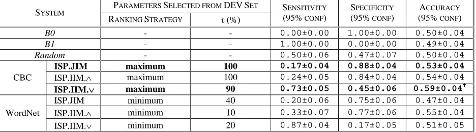
Table 1. Filtering quality of best performing systems according to the evaluation criteria defined in Section 4.3 on the TEST set – the reported systems were selected based on the Accuracy criterion on the DEV set.

PARAMETERS SELECTED FROM DEV SET SYSTEM

RANKING STRATEGY τ (%)

SENSITIVITY (95% CONF)

SPECIFICITY (95% CONF)

ACCURACY (95% CONF)

B0 - - 0.00±0.00 1.00±0.00 0.50±0.04

B1 - - 1.00±0.00 0.00±0.00 0.49±0.04

Random - - 0.50±0.06 0.47±0.07 0.50±0.04

ISP.JIM maximum 100 0.17±0.04 0.88±0.04 0.53±0.04

ISP.IIM.∧ maximum 100 0.24±0.05 0.84±0.04 0.54±0.04

CBC

ISP.IIM.∨ maximum 90 0.73±0.05 0.45±0.06 0.59±0.04†

ISP.JIM minimum 40 0.20±0.06 0.75±0.06 0.47±0.04

ISP.IIM.∧ minimum 10 0.33±0.07 0.77±0.06 0.55±0.04

WordNet

ISP.IIM.∨ minimum 20 0.87±0.04 0.17±0.05 0.51±0.05 †

5.2 Filtering Quality

For each ISP algorithm and parameter

combina-tion, we constructed a confusion matrix on the de-velopment set and computed the system sensitivity, specificity and accuracy as described in Section 4.3. This resulted in 180 experiments on the

devel-opment set. For each ISP algorithm and semantic

class source, we selected the best parameter com-binations according to the following criteria:

•Accuracy: This system has the best overall abil-ity to correctly accept and reject inferences.

•90%-Specificity: Several formal semantics and textual entailment researchers have commented that inference rule collections like DIRT are dif-ficult to use due to low precision. Many have asked for filtered versions that remove incorrect inferences even at the cost of removing correct inferences. In response, we show results for the system achieving the best sensitivity while main-taining at least 90% specificity on the DEV set. We evaluated the selected systems on the TEST set. Table 1 summarizes the quality of the systems

selected according to the Accuracy criterion. The

best performing system, ISP.IIM.∨, performed

sta-tistically significantly better than all three

base-lines. The best system according to the

90%-Specificity criteria was ISP.JIM, which coinciden-tally has the highest accuracy for that model as

shown in Table 16. This result is very promising

for researchers that require highly accurate

infer-ence rules since they can use ISP.JIM and expect to

recall 17% of the correct inferences by only ac-cepting false positives 12% of the time.

Performance and Error Analysis

Figures 1a) and 1b) present the full confusion ma-trices for the most accurate and highly specific sys-tems, with both systems selected on the DEV set.

The most accurate system was ISP.IIM.∨, which is

the most permissive of the algorithms. This

6

The reported sensitivity of ISP.Joint in Table 1 is below 90%, however it achieved 90.7% on the DEV set.

gests that a larger corpus for learning SPs may be needed to support stronger performance on the more restrictive methods. The system in Figure 1b), selected for maximizing sensitivity while maintaining high specificity, was 70% correct in predicting correct inferences.

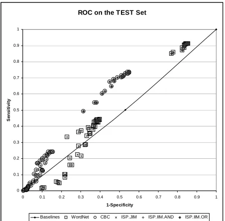
Figure 2 illustrates the ROC curve for all our systems and parameter combinations on the TEST set. ROC curves plot the true positive rate against the false positive rate. The near-diagonal line plots the three baseline systems.

Several trends can be observed from this figure. First, systems using the semantic classes from WordNet tend to perform less well than systems using CBC classes. As discussed in Section 4.2, we used a very simplistic extraction of semantic classes from WordNet. The results in Figure 2 serve as a lower bound on what could be achieved with a better extraction from WordNet. Upon in-spection of instances that WordNet got incorrect but CBC got correct, it seemed that CBC had a much higher lexical coverage than WordNet. For example, several of the instances contained proper

names as either the X or Y argument (WordNet has

poor proper name coverage). When an argument is not covered by any class, the inference is rejected.

Figure 2 also illustrates how our three different

ISP algorithms behave. The strictest filters, ISP.JIM

and ISP.IIM.∧, have the poorest overall perform-ance but, as expected, have a generally very low

rate of false positives. ISP.IIM.∨, which is a much

more permissive filter because it does not require

ROC on the TEST Set

0 0.1 0.2 0.3 0.4 0.5 0.6 0.7 0.8 0.9 1

0 0.1 0.2 0.3 0.4 0.5 0.6 0.7 0.8 0.9 1

1-Specificity

S

e

n

s

it

iv

it

y

[image:7.612.314.540.60.282.2]

Baselines WordNet CBC ISP.JIM ISP.IIM.AND ISP.IIM.OR

Figure 2. ROC curves for our systems on TEST.

GOLD STANDARD a)

1 0 1 184 139

S

YSTEM _{0 63 114}

GOLD STANDARD b)

1 0 1 42 28

S

[image:7.612.73.302.60.121.2]

YSTEM _{0 205 225}

Figure 1. Confusion matrices for a) ISP.IIM.∨ – best

both arguments of a relation to match, has gener-ally many more false positives but has an overall better performance.

We did not include in Figure 2 an analysis of the

minimum, maximum, and average ranking strate-gies presented in Section 3.2 since they generally produced nearly identical results.

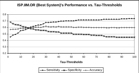
For the most accurate system, ISP.IIM.∨, we

ex-plored the impact of the cutoff threshold τ on the

sensitivity, specificity, and accuracy, as shown in Figure 3. Rather than step the values by 10% as we did on the DEV set, here we stepped the threshold value by 2% on the TEST set. The more

permis-sive values of τ increase sensitivity at the expense

of specificity. Interestingly, the overall accuracy remained fairly constant across the entire range of

τ, staying within 0.05 of the maximum of 0.62

achieved at τ=30%.

Finally, we manually inspected several incorrect inferences that were missed by our filters. A com-mon source of errors was due to the many incorrect “antonymy” inference rules generated by DIRT,

such as “X is rejected in Y”⇒“X is accepted in Y”.

This recognized problem in DIRT occurs because of the distributional hypothesis assumption used to

form the inference rules. Our ISP algorithms suffer

from a similar quandary since, typically, antony-mous relations take the same sets of arguments for

X (and Y). For these cases, ISP algorithms learn

many selectional preferences that accept the same types of entities as those that made DIRT learn the

inference rule in the first place, hence ISP will not

filter out many incorrect inferences.

6

Conclusion

We presented algorithms for learning what we call inferential selectional preferences, and presented

evidence that learning selectional preferences can be useful in filtering out incorrect inferences. Fu-ture work in this direction includes further explora-tion of the appropriate inventory of semantic classes used as SP’s. This work constitutes a step towards better understanding of the interaction of selectional preferences and inferences, bridging these two aspects of semantics.

References

Barzilay, R.; and McKeown, K.R. 2001.Extracting Paraphrases from a Parallel Corpus. In Proceedings of ACL 2001. pp. 50–57. Toulose, France.

Baker, C.F.; Fillmore, C.J.; and Lowe, J.B. 1998. The Berkeley FrameNet Project. In Proceedings of COLING/ACL 1998. pp. 86-90. Montreal, Canada.

Cover, T.M. and Thomas, J.A. 1991. Elements of Information Theory. John Wiley & Sons.

Fellbaum, C. 1998. WordNet: An Electronic Lexical Database. MIT Press.

Harabagiu, S.; and Hickl, A. 2006. Methods for Using Textual Entailment in Open-Domain Question Answering. In Proceedings of ACL 2006. pp. 905-912. Sydney, Australia.

Katz, J.; and Fodor, J.A. 1963. The Structure of a Semantic Theory. Language, vol 39. pp.170–210.

Lenat, D. 1995. CYC: A large-scale investment in knowledge infrastructure. Communications of the ACM, 38(11):33–38.

Levin, B. 1993. English Verb Classes and Alternations: A Preliminary Investigation. University of Chicago Press, Chicago, IL.

Light, M. and Greiff, W.R. 2002. Statistical Models for the Induction and Use of Selectional Preferences. Cognitive Science,26:269–281. Lin, D. 1993. Parsing Without OverGeneration. In Proceedings of

ACL-93. pp. 112-120. Columbus, OH.

Lin, D. and Pantel, P. 2001. Discovery of Inference Rules for Question Answering. Natural Language Engineering 7(4):343-360. Moldovan, D.I.; Clark, C.; Harabagiu, S.M.; Maiorano, S.J. 2003.

COGEX: A Logic Prover for Question Answering. In Proceedings ofHLT-NAACL-03. pp. 87-93. Edmonton, Canada.

Pantel, P. and Lin, D. 2002. Discovering Word Senses from Text. In Proceedings of KDD-02. pp. 613-619. Edmonton, Canada.

Resnik, P. 1996. Selectional Constraints: An Information-Theoretic Model and its Computational Realization. Cognition, 61:127–159. Romano, L.; Kouylekov, M.; Szpektor, I.; Dagan, I.; Lavelli, A. 2006.

Investigating a Generic Paraphrase-Based Approach for Relation Extraction. In EACL-2006. pp. 409-416. Trento, Italy.

Rosch, E. 1978. Human Categorization. In E. Rosch and B.B. Lloyd (eds.) Cognition and Categorization. Hillsdale, NJ: Erlbaum. Siegel, S. and Castellan Jr., N. J. 1988. Nonparametric Statistics for

the Behavioral Sciences. McGraw-Hill.

Szpektor, I.; Tanev, H.; Dagan, I.; and Coppola, B. 2004. Scaling web-based acquisition of entailment relations. In Proceedings of EMNLP 2004.pp. 41-48. Barcelona,Spain.

Wilks, Y.; and Fass, D. 1992. Preference Semantics: a family history. Computing and Mathematics with Applications, 23(2). A shorter version in the second edition of the Encyclopedia of Artificial Intelligence, (ed.) S. Shapiro.

[image:8.612.74.297.62.179.2]

Zanzotto, F.M.; Pennacchiotti, M.; Pazienza, M.T. 2006. Discovering Asymmetric Entailment Relations between Verbs using Selectional Preferences. In COLING/ACL-06. pp. 849-856. Sydney, Australia.

Figure 3. ISP.IIM.∨ (Best System)’s performance

variation over different values for the τ threshold. ISP.IIM.OR (Best System)'s Performance vs. Tau-Thresholds

0.2 0.3 0.4 0.5 0.6 0.7 0.8

0 10 20 30 40 50 60 70 80 90 100

Tau-Thresholds