Design of Self Assembling Molecules and Boundary Value Problem for Flows on a Space of n Simplices

(1)

ISSN Online: 2152-7393 ISSN Print: 2152-7385

DOI: 10.4236/am.2019.1011065 Nov. 11, 2019 907 Applied Mathematics

Design of Self-Assembling Molecules and

Boundary Value Problem for Flows on a

Space of

n

-Simplices

Naoto Morikawa

Genocript, Zama, Japan

Abstract

Self-assembling molecules are ubiquitous in nature, among which are pro-teins, nucleic acids (DNA and RNA), peptides and lipids. Recognizing the ability of biomolecules to self-assemble into various 3D shapes at the nanos-cale, researchers are mimicking the self-assembly strategy for engineering of complex nanostructures. However, the general principles underlying the de-sign of self-assembled molecules have not yet been identified. The question is “How to obtain a well-defined shape with desired properties by folding a chain of subunits (such as amino acids and nucleic acids)”, where properties are determined by the precise spatial arrangement of the subunits on the sur-face. In this paper, we consider the question from the viewpoint of the dis-crete differential geometry of n-simplices. Self-assembling molecules are then represented as a union of trajectories of 3-simplices (i.e., tetrahedrons), and the question is rephrased as a “boundary value problem” for flows on a space of tetrahedrons. Also considered is a characterization of two types of surface flows of n-simplices. It is a rough classification of surface flows, but may be essential in characterizing important properties of biomolecules such as allosteric regulation. The author believes this paper not only provides a new perspective for the engineering of self-assembling molecules, but also promotes further collaboration between mathematics and other disciplines in life science.

Keywords

Differential Geometry, Self-Assembling Molecule, Discrete Mathematics, Boundary Value Problem, Flows of n-Simplices

1. Introduction

Self-assembling molecules are ubiquitous in nature, among which are proteins,

How to cite this paper: Morikawa, N. (2019) Design of Self-Assembling Mole-cules and Boundary Value Problem for Flows on a Space of n-Simplices. Applied Mathematics, 10, 907-946.

https://doi.org/10.4236/am.2019.1011065

Received: October 6, 2019 Accepted: November 8, 2019 Published: November 11, 2019

http://creativecommons.org/licenses/by/4.0/

(2)

DOI: 10.4236/am.2019.1011065 908 Applied Mathematics nucleic acids (DNA and RNA), peptides and lipids. Recognizing the ability of biomolecules to self-assemble into various 3D shapes at the nanoscale, re-searchers are mimicking the bottom-up self-assembly strategy for precise engi-neering of complex nanostructures [1] [2] [3]. As suggested by Gellman in [3], “realization of the potential of folding polymers may be limited more by the human imagination than by physical barriers”.

However, we have not yet identified the underlying general principles that govern the engineering of self-assembling molecules. The question is

“How to obtain a well-defined shape with desired properties by folding a chain of subunits,”

where properties are determined by the precise spatial arrangement of the sub-units on the surface. In the case of proteins, on the surface are “active sites” formed by a set of amino acids arranged in a specific configuration, through which proteins carry out their function. Note that a pair of subunits adjacent on the surface are often far apart along the chain.

The question shown above is divided into two sub-questions. One is to find a backbone conformation called targetstructure that forms a shape of the desired properties. The other is to find a chain of subunits that adopts the target struc-ture. In this paper, we shall discuss the former of these two sub-questions from the viewpoint of the discrete differential geometry of n-simplices.

Using the mathematical toy model proposed in [4] [5], we shall represent self-assembling molecules as a union of trajectories of 3-simplices (i.e., tetrahe-drons). Then, the former sub-question is rephrased as a “boundary value prob-lem” for flows on a space of 3-simplices:

“Given a triangular flow (i.e., desired properties). Find a tetrahedral flow (i.e., well-defined shape) that induces the triangular flow as its surface flow.”

In this paper, we first give an introduction to the discrete differential geome-try of n-simplices. In addition to the case of triangles and tetrahedrons, we also consider the case of 1-simplices (line segments) in order to handle surface flows induced on a union of trajectories of triangles. After giving a definition of boundary value problem for flows on a space of n-simplices, we shall consider the boundary value problem with some examples. For simplicity, we mainly deal with flows of triangles and their surface flows of line segments. Finally given is a characterization of two types of surface flows of line segments, i.e., _3_-embeddable surface flow and locally _3_{-embeddable surface flow. This distinction may} be essential in characterizing some important properties of biomolecules such as “allosteric regulation” (i.e., long distance interactions between subunits) as men-sioned in [5]. Some open problems are also given along the way.

We believe this paper will open up a new perspective for the engineering of self-assembling molecules and bring about further advances in collaboration between mathematics and other disciplines in life science.

(3)

DOI: 10.4236/am.2019.1011065 909 Applied Mathematics structure analysis. In particular, the author is not affiliated with any research in-stitution.

2. Previous Works

Actively researched self-assembling molecules include biomolecules such as DNA (i.e., polynucleotides), proteins (i.e., polypeptides), and unnatural molecules such as foldamers (i.e., unnatural oligomers). As for approaches from mathe-matics, there are no known attempts other than sporadic applications of graph theory in the engineering of DNA- and protein-based nanostructures.

2.1. DNA-Based Nanostructures

Self-assembling DNA-based nanostructures have been extensively studied, as the specificity of Watson-Crick base pairing provides ease of control over interac-tions between DNA strands. Well known in the field of DNA nanotechnology is the scaffolded DNA origami method [1], in which a long single-stranded DNA (called scaffold strand) is folded into arbitrary shapes with the help of many short single-stranded DNAs (called staplestrands) in a single step.

For two-dimensional shapes, a target shape is approximated by folding a scaf-fold strand back and forth in a raster fill pattern. The target shape is then ob-tained as a flat sheet of antiparallel DNA double helices which is cross-linked by lots of staple strands.

Three-dimensional shapes are obtained by stacking flat sheets of antiparallel DNA double helices to form a closely packed pleated layer structure [6]. To con-struct space-filling multilayer objects, flat sheets are packed onto a honeycomb lattice, a square lattice, or a hexagonal lattice [7].

2.2. Protein-Based Nanostructures

Protein-based nanostructures have several advantages over DNA-based nano-structures, such as structural richness, functional versatility, and cost effective manufacturing. DNA-based nanostructures consist of four nucleic acids, and are prepared by chemical synthesis. In contrast, protein-based nanostructures con-sist of 20 amino acids, and are manufactured by biotechnological methods. One of the disadvantages is the much more complicated design rules, due to the con-tribution of many cooperative and long range interactions between amino acids. There are two types of approaches in finding a polypeptide that folds into a specified 3D shape (i.e., protein design). One is the design of proteins with a de-sired backbone structure. The other is the design of proteins with dede-sired func-tions (i.e., desired active sites or desired interacting surfaces).

(4)

DOI: 10.4236/am.2019.1011065 910 Applied Mathematics A set of target backbone structures consistent with the diagram are often gen-erated by assembling short backbone fragments from existing proteins [10] [11] [12]. Note that it is not clear whether the target structure is designable, i.e., there exists an amino acid sequence that would adopt the conformation in nature. By reusing naturally occurring protein fragments, it is ensured that new backbone structures are more likely to be designable.

On the other hand, functional design generally starts with a target active site or a target interacting surface description. A target active site description in-cludes a target reaction and a model of the reaction mechanism [13]. Active sites usually consist of functional residues located in different regions (i.e., disjoint fragments) of the linear polypeptide chain. A three-dimensional arrangement of the functional residues is derived from the given description. A set of existing proteins is then searched for backbones that can support the arrangement of the functional residues [14] [15], onto which the target active site is grafted. For now, it is difficult to generate new backbones from a set of disjoint fragments so that the resulting backbone accommodates the spatial arrangement of the given set of disjoint fragments [12].

2.3. Protein Origami

In addition, there is another approach to constructing self-assembled protein nanostructures, called “protein origami” [2] [16]. This approcach is based on the specificity of pairwise interactions between coiled-coil-forming polypeptide segments rather than the numerous cooperative interactions between amino ac-ids. The coiled-coils are composed of two intertwined helical segments that wrap around each other to form a supercoiled structure, where each segment binds only to its designated partner and does not interact with the others (i.e., ortho-gonal).

The orthogonal coiled-coil-forming segments are concatenated in a specified order to form a single polypeptide chain, which folds into a polypeptide polyhe-dron as the orthogonal interacting segments assemble into coiled-coils with their designated partners. For example, a tetrahedron is self-assembled from a poly-peptide chain consisting of 12 coiled-coil forming segments separated by flexible linkers. The generated 6 coiled-coils correspond to the 6 edges, and the linkers are located on the vertices. The sequential arrangement of the 12 coiled-coil forming segments and the orientation of each coiled-coil pair are obtained as a double Eulerian path in a tetrahedron, i.e. an oriented path that traverse each of the 6 edges of the tetrahedron exactly twice. The existence of double Eulerian paths is guaranteed by graph theory, because all the vertices of a double tetrahe-dral graph have an even degree.

2.4. Unnatural Molecules

(5)

DOI: 10.4236/am.2019.1011065 911 Applied Mathematics not found in nature.

Most of the research so far has focused on reproducing local structural pat-terns of proteins such as helices and sheets [17] [18] [19]. It is still a major chal-lenge to pack the local structural patterns obtained into a uniquely specified compact conformations [20].

So far no foldamaer is known that displays a given compact conformations [21]. Natural proteins typically require more than 100 residues to display sta-ble compact conformation. However, careful choice of preorganized mono-mers may lead to foldamono-mers of less than 40 residues with stable compact con-formation [3].

2.5. Flows of

n

-Simplices

The author is unaware of similar studies by other researchers on flows of n-simplices.

As for differential geometry on a space of n-simplices, differential geometry on polyhedra (such as differential forms on n-simplices) has been studied from the view point of classification of geometrical objects (For example, see [22]). In particular, n-simplices have been played an important role in homological alge-bra [23]. However, shapes of trajectories of n-simplices are not explicitly consi-dered there.

As for surfaces consisting of triangles, they have been studied as discrete ana-logues of smooth geometric objects [24]. Typically, they are obtained as a result of the triangulation of the surfaces of real world objects in 3D computer graphics. However, there are no known studies on flows of triangles on the triangular sur-face.

3. Flows of

n

-Simplices

This paper proposes a novel mathematical approach for the design of self-assembling molecules, which is based on the discrete differential geometry of n-simplices [4] [5]. In our approach, self-assembling molecules are represented as a union of trajectories of tetrahedrons. The “spatial arrangement of the subunits (such as amino acids, nucleic acids, or others)” on the surface of a molecule then corresponds to the “flow of triangles” induced on the surface of a union of tra-jectories of tetrahedrons. In this section, we shall give an introduction to the discrete differential geometry of n-simplices.

In the following,  denotes the set of all natural numbers,  denotes the set of all integers,  denotes the set of all real numbers, and _En₍_n_∈_₎

de-notes the n-dimensional Euclidean space.

For space saving purposes, the coordinates of points in _En_{are represented}

by a monomial in n indeterminates x x0, , ,1 xn−1. For example, point

(

_{l m n E}_{, ,}

)

_∈ 3_{is represented by} 0 1l m n2

x x x . Points

(

0,0,0

)

,

(

0,0,n

)

,

(

0, ,m n

)

are represented by 1, x2n, x x1m n2 , respectively. Moreover, px0k denotes the point

(

_{l k m n E}₊ _{, ,}

)

_∈ 3_{, where}

0 1l m n2

(6)

DOI: 10.4236/am.2019.1011065 912 Applied Mathematics

3.1. General Case

3.1.1. Flows on an n-Simplex Space

First of all, we shall define a space of n-simplices, upon which flows of n-simplices are defined. The topology of the space is defined using “adjacent” rela-tionship between n-simplices.

Definition 1 (n-simplex). Let n∈__{. An}_n-simplex_{is the convex hull of}

(

n+1

)

_{affinely independent points in} _En₍_i_._e_{., points not lying in a}

(

_n₋₁

)

_-di-

mensional subspace). The convex hull of n+1_points ₀, , ,₁ n n

v v v ∈E is de-noted by

[

v v0, , ,1 vn

]

, i.e.,

[

0 1

]

0,1, , 0,1, ,

, , , : i n| 1 and , 0 .

n i i i

i n i n

v v v vλ E _λ i _λ

= =

 

=_ ∈ = ∀ ≥ _



∏

∑



Then, vi (0≤ ≤i n) are called the vertices of

[

v v0, , ,1 vn

]

. Let s be an

n-simplex. The set of all the vertices of s is denoted by v s

( )

.

For example, a 0-simplex is a point, a 1-simplex is a line segment, a 2-simplex is a triangle, a 3-simplex is a tetrahedron.

Definition 2 (k-face). Let k n, ∈ and k n≤ _{. Let s be an}_n_{-simplex. A} k-face of s is the convex hull of any k+1_{vertices of}_s_{. A 0-face is a vertex of}_s_.

A 1-face is called an edge of s. An

(

n−1

)

_{-face is called a}_facet_of_s_{. Note that the}

n-face is s itself.

For example, let s=

[

v v v v0, , ,1 2 3

]

be a tetrahedron. Then, s has 6 edges

,

i j

v v

 

  (0≤ < ≤i j 3) and 4 facets v v vi, ,j k (0≤ < < ≤i j k 3). Moreover,

( ) {

0, , ,1 2 3

}

v s = v v v v .

Definition 3 (n-simplex space). Let M be a set of n-simplices. M is called an n-simplex space if each n-simplex is connected to other n-simplices in such a way that,

for ∀_{facet u of} s M∈ _{, uniquely} s M′∈ _{such that} s s∩ ′ =u.

In particular, each n-simplex is connected to n+1_{“adjacent”}_n_-simplices through its n+1_facets.

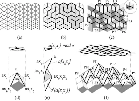
Example 1. We would obtain an n-simplex space by partitioning _En_into

pieces of n-simplices. Shown in Figure 1(a) is a triangle space M0 obtained by partitioning _E2_{into pieces of triangles.}

Definition 4 (k-face neighborhood N(u)). Let M be an n-simplex space and

s M∈ _{. Let}_u_{be a}_k_{-face of}_s_{. The}_k-face_neighborhood N u

( )

of u is a set of n-simplices of M which contain u:

( ) {

: |

}

.

N u = s M u s′∈ ⊂ ′

For s=

[

v v0, , ,1 vn

]

∈M , we obtain s=

∩

i=0,1, ,nN v

( )

i . Note that every facet neighborhood consists of two n-simplices. We shall use the fact when de-fining local trajectories of n-simplices (See just above Definition 6).

Now let us define flows of n-simpleces on an n-simplex space.

Definition 5 (Tangent space T(s)). Let s be an n-simplex. The tangent space

( )

(7)

[image:7.595.262.484.65.280.2]

DOI: 10.4236/am.2019.1011065 913 Applied Mathematics Figure 1. Flow of triangles. (a) A triangle space M0 obtained by partitioning E2 into pieces of triangles; (b) Gradients of triangles of M0. For each triangle s M∈ 0, the gradient (i.e., the set of edges assigned) is drawn with thick lines. The white arrow indicates the position of the triangle s0 (grey) of (c); (c) Shown left is a triangle s0 (grey) and three adjacent triangles (white) connected to s0 through three facets. Shown in the square frame are all the possible values of the gradient of s0 and the adjacent triangles associated with the value. From left to right, a branch triangle, three regular triangles, three 2-fold singular triangles (terminal triangles), a 3-fold singular triangle (isolated triangle). Enclosed by a dotted circle is the gradient of s0 of (b).

( )

:

{

j, j | 0

}

,

T s = _v v _ ≤ < ≤i j n

where v s

( ) {

= v v0, , ,1 vn

}

. A subset of T s

( )

is called a gradient of s.

Example 2. In Figure 1(b), a gradient (i.e., a set of edges) is assigned to each triangle of M0. Most of the triangles are assigned one edge, some are assigned multiple edges, and others are assigned no edge. Shown in Figure 1(c) are all the possible values of the gradient of a triangle s0 of M0, from which the encir-cled value is assigned to s0 in (b).

Let M be an n-simplex space. Let s=

[

v v0, , ,1 vn

]

∈M and

[

a, b

]

( )

e= v v ∈T s . Two facets u s ea

( )

, and u s eb

( )

, of s which do not

con-tain the edge e are defined by

( )

0

, , , , , ,

a a n

b b n

u s e v v v

 ₌ 

  



 

=

 _ _



where means that the corresponding term is omitted.

Then, by definition, there are two n-simplices s s ea

( )

, and s s eb

( )

, ∈M

such that

( )

(

)

{

( )

}

( )

(

,,

)

{

,,

( )

,,

}

.,

a a

b b

N u s e s s s e

 =

 

(8)

DOI: 10.4236/am.2019.1011065 914 Applied Mathematics Definition 6 (Adjacent n-simplices A(s,G)). Let M be an n-simplex space. Let

s M∈ _and e T s∈

( )

. The adjacentn-simplices A s e

( )

, associatedwiththeedge eofs is defined by

( )

, :

{

a

( ) ( )

, , b ,

}

,

A s e = s s e s s e

where s s e_a

( )

, and s s e_b

( )

, are defined above. That is, A s e

( )

, is the set of all the adjacent triangles of s which do not contain the edge e.

Let G T s⊂

( )

_{be a gradient of}_s_{. The}_adjacent _n-simplices A s G

(

,

)

asso-ciatedwithG is defined by

(

,

)

:

( )

, , if

all the adjacent -simplices of , if

e GA s e G

A s G

n s G

∈

 ≠ ∅

 = 

= ∅ 

∩

In particular A s e

( )

, =

{

s A e′∈

(

,∅

)

|e s⊂/ ′

}

.

Definition 7 (Local trajectory at an n-simplex). Let M be an n-simplex space. Let s M∈ _and e T s∈

( )

_{. Let} A s e

( ) {

, = s s_a, _b

}

_{. The}_local_trajectory _at _s

asso-ciatedwiththeedgee is the sequence

(

or

)

a b b a

s − −s s s − −s s

of three consecutive n-simplices. Connecting these sequences together, we shall obtain a flow on M in Definition 12 and 13.

Example 3. Grey triangles in Figure 1(c) are the adjacent triangles A s G

(

0,

)

associated with the gradient G (thick lines) of s0.

Conversely, a sequence s0− −s s2 of three consecutive n-simplices determines uniquely an edge of the middle n-simplex s as follows.

Definition 8 (Tangent D st

(

0− −s s2

)

). Let M be an n-simplex space. Let

0 2

s − −s s _{be a sequence of three consecutive}_n_{-simplices of}_M_,_i_._e_.,

(

)

0, 2 ,

s s ∈A s ∅ _{such that} s₀≠s₂_{. Let}

(

)

(

)

0 0 0

2 2 2

: the facet shared by and ,

: the facet shared by and .

u s s s s

 =   ₌ 

∩ ∩

The tangent D st

(

0− −s s2

)

to s0− −s s2 at s is an edge

[

v v0, 2

]

of s, where

( ) ( ) (

)

( ) ( ) (

)

0 0 0

2 2 2

: \ the vertex not included in ,

: \ the vertex not included in .

v v s v u u

 =   ₌ 

Note that Dt is not defined at singular simplices because singular simplices never occupy the middle position of a sequence of three consecutive n-simplices. (See Figure 1(c).)

Lemma 1. Let M be an n-simplex space. Let s M∈ _and e T s∈

( )

_{. Let}

0 2

s − −s s _{be a sequence of three consecutive}_n_{-simplices of}_M_{. Then,}

(

)

(

)

{

}

( )

(

, ,0 2 ,

)

0, 2 ,

(

( )

,

( )

,

)

,

t

t a b t b a

A s D s s s s s

D s s e s s s e D s s e s s s e e

 − − =

 

− − = − − =



where s s ea

( )

, and s s eb

( )

, are the two n-simplices of A s e

( )

, .

Proof. It follows immediately from the definition.

(9)

DOI: 10.4236/am.2019.1011065 915 Applied Mathematics Definition 9 (Tangent bundle

(

TM M, ,π_M

)

_{). Let}_M_{be an}_n_{-simplex space.} The tangent bundle

(

TM M, ,π_M

)

_of_M_{is defined by}

( )

{

}

( )

: , | , ,

: , , : .

M

TM s u s M u T s

TM M s u s

π π

 = ∈ ∈

 

→ =



Definition 10 (Vector field V on M). Let M be an n-simplex space. A vector fieldV on M is a mapping which assigns to each n-simplex s of M, a gradient of s, i.e.,

( )

₍

_[

_]

₎

{

_[

_]

}

0 1

: 2 ,T s , , , , , , , ,

n i j k l

V M → V v v v _{= }v v _ v v

where 2T s( )_{denotes the power set of} _{T s}

_{( )}

_{. If} _{V s}

_{( )}

_{contains only one edge,}_s is called a regularn-simplex of V. Otherwise, s is called a singularn-simplex of V. If V s

( )

= ∅_,_s_{is called a}_branch_n_{-simplex of}_V_{. If}V s

( )

consists of m edges, s is called an m-foldsingularn-simplex of V. If A s V s

(

,

( )

)

has only one n-simplex, s is called a terminaln-simplex of V. If A s V s

(

,

( )

)

= ∅, s is called an iso-latedn-simplex.

Example 4. Shown in Figure 1(b) is a vector field of the triangle space M0 of (a).

Definition 11 (Local trajectory of V on M). Let M be an n-simplex space and

s M∈ _{. Let}_V_{be a vector field of}_M_{. Let} s₀− −s s₂_{be a sequence of three}

con-secutive n-simplices. Then, s0− −s s2 is called a localtrajectoryofV at s if

(

0 2

)

( )

.

t

D s − −s s ⊃V s

Note that local trajectories may contain branch n-simplices.

Definition 12 (Trajectory of V on M). Let M be an n-simplex space. Let V be a vector field of M. Let L=

{

s i i I

[ ]

| ∈ ⊂

}

be a sequence of n-simplices, where I is either

[

k m,

]

,

[

k,+∞

)

_,

(

−∞,m

]

_{, or}

(

−∞ +∞,

)

₍k m, ∈__{such that}

k m< _{). Then,}_L_{is called a trajectory of}_V_{if every consecutive three}_n_-simplices of L is a local trajectory of V. i.e.,

[ ] [ ] [

1 2 is a local trajectory of for

]

[

, 2

]

.

s i s i− + −s i+ V ∀i i+ ⊂I

A trajectory L=

{

s i i k m

[ ]

| ∈

[

,

]

⊂

}

of V is called closed if

[

1

] [ ] [ ]

and

[ ] [ ] [

1

]

s m− −s m s k− s m s k− −s k+ are also local trajectories of V.

A trajectory L of V is called maximal if either L is closed, or L′ ⊃L implies

L L′ = for any trajectory L′_of_V_on_M_.

Definition 13 (Flow of V on M). Let M be an n-simplex space. Let V be a vector field of M. Let F=

{

L i Ii| ∈ ⊂

}

be a set of maximal trajectories of V

on M, where Li ≠Lj if i≠ j. Then, L is called a flow of V on M if

.

i i I

M L

∈

=

_∪

(10)

DOI: 10.4236/am.2019.1011065 916 Applied Mathematics 3.1.2. Two Functions on a Trajectory

Here we define two functions on trajectories of vector fields on an n-simplex space.

Definition 14 (U/D function g along a trajectory). Let M be an n-simplex space. Let V be a vector field of M. Let L=

{

s

[ ] [ ]

0 , 1 , ,s s k

[ ]

}

(k∈__{) be a} trajectory of V on M. An U/DfunctiongalongL is a

{

+ −1, 1

}

-valued function on L defined by

[ ]

( )

{

}

[ ]

(

)

( )

_{( )}

[ ]

_{[ ]}

(

[ ]

)

( )

[ ]

0 1, 1 ,

, if 1

1 :

, otherwise

g s

g s i V s i V s i

g s i

 ∈ + − ⊂

 _

+ = ∅

 _

+ _{= }

 ₋



 



∩ 

Example 5. Shown in Figure 2 is a trajectory

[ ] [ ] [ ] [ ] [ ]

{

0 , 1 , 2 , 3 , 4 ,

}

a

L = s s s s s of the vector field of M0 given in Figure

1(b), where s

[ ]

0 =s0. Then, we obtain an U/D function ga along La as fol-lows: Firstly, set g sa

( )

[ ]

0 = +1 and move to the adjacent triangle s

[ ]

1 on the right. Then, g sa

( )

[ ]

1 = −g sa

( )

[ ]

0 = −1 since V s

( )

[ ]

1 ∩V s

( )

[ ]

0 ≠ ∅. In the same way, we obtain g sa

(

[ ]

2

)

= −g sa

( )

[ ]

1 = +1. Now, let us move to s

[ ]

3 . Then, g sa

( )

[ ]

3 =g sa

( )

[ ]

2 = +1 since V s

( )

[ ]

3 ∩V s

( )

[ ]

2 = ∅ . In the same way, we obtain g sa

( )

[ ]

4 =g sa

( )

[ ]

3 = +1.

By considering the “integral along the trajectory” of a given U/D function, we shall obtain another function on the trajectory.

Definition 15 (Height function hg on a trajectory). Let M be an n-simplex

space. Let V be a vector field of M. Let L=

{

s

[ ] [ ]

0 , 1 , ,s s k

[ ]

}

(k∈) be a trajectory of V on M. Let g be a U/D function along L. The heightfunction hg

withrespecttog is a -valued function on L defined by

[ ]

(

)

[ ]

(

)

( )

_{( )}

[ ]

_{[ ]}

( )

[ ]

(

[ ]

)

( )

[ ]

0 ,

, if 1

1 :

, otherwise

g

g g

g

h s

h s i g s i V s i V s i

h s i

 ∈

 _

+ + = ∅

 ₊ 

=  



 



∩ 

Figure 2. Two functions on a trajectory of triangles. Shown on the left is a trajectory

[ ] [ ] [ ] [ ] [ ]

{

0 , 1 , 2 , 3 , 4 ,

}

a

L = s s s s s of the vector field of M0 given in Figure 1(b), where

[ ]

0 0

[image:10.595.238.510.479.658.2]

(11)

DOI: 10.4236/am.2019.1011065 917 Applied Mathematics Example 6. Shown in Figure 2 is a trajectory

[ ] [ ] [ ] [ ] [ ]

{

0 , 1 , 2 , 3 , 4 ,

}

a

L = s s s s s of the vector field of M0 given in Figure

1(b), where s

[ ]

0 =s0. The table on the right shows the values of an U/D func-tion ga along La (See Example 5) and the height function hga with respect to ga. hga is obtained as follows: Firstly, set h sga

(

[ ]

0

)

=0. Since

[ ]

( )

1

( )

[ ]

0

V s ∩V s ≠ ∅, we obtain h sg

( )

[ ]

1 =h sg

( )

[ ]

0 =0. In the same way, we obtain h sg

( )

[ ]

2 =h sg

( )

[ ]

1 =0. Now, let us move to s

[ ]

3 . Then,

[ ]

( )

3

( )

[ ]

2

V s ∩V s = ∅ and

[ ]

( )

3

( )

[ ]

2

( )

[ ]

3 0 1 1.

g g

h s =h s +g s = + =

In the same way, we obtain h sg

( )

[ ]

4 =h sg

( )

[ ]

3 +g s

( )

[ ]

4 =2.

3.2. Flows of

_n+1

_{-Embeddable Vector Fileds}

In general, n-simplex spaces consist of n-simplices of various shapes. Here, we shall consider a special class of n-simplex spaces consisting of n-simplices of the same shape.

3.2.1. _3_{-Embeddable Vector Fields of Triangles}

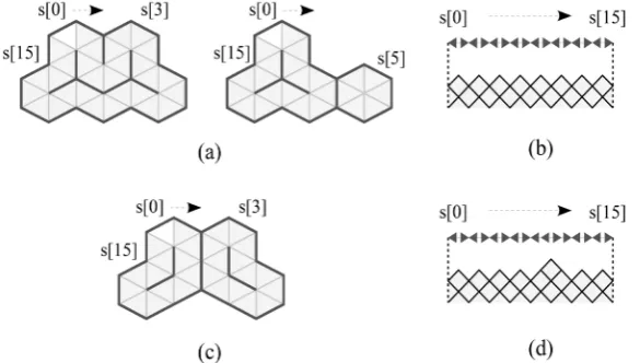
Shown in Figure 3(a) is a triangle space M1 obtained by partitioning E2 into triangles of the same shape. A vector field on M1 is shown in Figure 3(b). In this case, the “two-dimensional” vector field of M1 corresponds to a “three- dimensional” drawing on the surface of “mountains” of unit cubes of _E3_as shown in Figure 3(c) and Figure 3(f). It is this type of vector fields of triangles that is considered in this section.

Definition 16 (The three-dimensional lattice _L3_{). Let} _L3_{be the three-di-} mensional lattice generated by three vectors

(

1,0,0

)

,

(

0,1,0

)

, and

(

0,0,1

)

, i.e.,

{

}

3 3

0 1 2

: l m n| , , .

L = x x x l m n∈ ⊂E

Shown in Figure 3(d) is a unit cube of _L3_{and its top view.}

Definition 17 (The symmetric group _Sym3_{on three letters). Let} _Sym3_be the group of all the permutations of the set

{

0,1,2

}

. Elements of _Sym3_are written in cyclic notation. For example, let

ρ

=

( )

021 ∈Sym3_{. Then,} ρ

_{( )}

0 =2_,

( )

1 0

ρ = , and ρ

( )

2 =1.

Definition 18 (The set B2 of all flat triangles). Let a L∈ 3 and ρ∈Sym3. The

slant triangle a x_ ρ( )0xρ( )1_ is defined by

( )0 ( )1 : , ( )0 , ( )0 ( )1 ,

a x x_ ρ ρ _ =_a axρ ax xρ ρ _

where

[

a b c, ,

]

denotes the convex hull of three points _{a b c E}_{, ,} _∈ 3_(Definition 1). For example, the four slant triangles shown in Figure 3(e) are a x x

[

0 1

]

,

[

]

0 1 2

(12)

[image:12.595.240.510.74.271.2]

DOI: 10.4236/am.2019.1011065 918 Applied Mathematics Figure 3. _3_{-embeddable vector field. (a) A triangle space}

1

M consisting of triangles of the same shape; (b) A vector field on M1. Three closed trajectories are colored differently; (c) The top view of “mountains” obtained by piling up unit cubes of _E3_in

the direction of

(

− − −1, 1, 1

)

. Shown in the circle is a unit cube, where each of the three upper faces is divided into two triangles by the vertical diagonal (thick line). The flow of triangles obtained by connecting thick lines corresponds to the flow of the vector field of (b); (d) A unit cube of _L3_{(bottom) and its top view (top); (e) The} _σ_{-equivalence class}

of a x x

[ ]

0 1 ; (f) Projection of the slant triangles on the surface of the “mountains” of (c)

(bottom) onto the triangle space M1 of (a) (top).

( ) ( )

{

3 3

}

2: 0 1 | , .

S = a x x_ ρ ρ _ a L∈ ρ∈Sym

The shiftoperator σ_on S₂ is defined by

( ) ( )

(

a x xρ0 ρ1

)

: axρ( )0 x xρ( )1 ρ( )2 .

σ _ _ = _ _

Then, an equivalence relation σ is defined on S2 by a b

t σ t if and only if ∃ ∈m s.t.

σ

m

( )

ta =tb.

The σ _{-equivalence class of}t S∈ ₂_{is called a}_flat_triangle_{and denoted by}

mod

t σ. For example, shown in Figure 3(e) is the σ -equivalence class of

[

0 1

]

mod

a x x σ ₍_{a L}_∈ 3_).

The set of all flat triangles is denoted by B2, i.e.,

2: 2 .

B =S σ Lemma 2. B2 is a triangle space (Definition 3).

Proof. It follows immediately from the definition.

By an abuse of notation, the “image on B2“ of an edge e of s S∈ 2 is also denoted by emodσ . Note that

[

a ax x, 0 1

]

modσ =

[

a ax x′, 0 1

]

modσ =

[

a a x x′ ′, 0 1

]

mod ,σ

where _{a L}_∈ 3_and

0 1 2

a ax x x′ = _(See_{Figure 3(e)}_{). The tangent space}

( ) ( )

(

0 1 mod

)

(13)

DOI: 10.4236/am.2019.1011065 919 Applied Mathematics ( ) ( )

(

)

( ) ( ) ( ) ( ) ( ) ( )

{

}

0 1

0 1 1 2 2 0

mod

, mod , , mod , , mod ,

T a x x

a ax x a a x x a a x x

ρ ρ

ρ ρ ρ ρ ρ ρ

σ

σ σ σ

 

 

   ′ ′   ′′ ′′ 

=      

where

a ax

′ =

ρ( )0 and

a ax x

′′ =

ρ( ) ( )0 ρ1 .

For simplicity, we often identify the edge a ax x, i jmodσ with the monomial

i j

x x and we shall obtain a one-to-one correspondence

( ) ( )

(

0 1 mod

)

{

0 1, 1 2, 0 2

}

.

T a x x ρ ρ  σ  x x x x x x

Definition 19 (Tangent bundle

(

TB B2, ,2 πB₂

)

). The tangent bundle of B2 (Definition 9) is given by

(

)

(

)

{

}

(

)

2 2 2 2 2 2

: mod , | mod , mod ,

: , mod , : mod .

B B

TB t u t B u T t

TB B t u t

σ σ σ

π π σ σ

 = ∈ ∈



 _→ ₌



Definition 20 (Gradient D tS ). Let t a x x=  ρ( )0 ρ( )1∈S2. The gradient D tS of t is defined by

( )0 ( )1

: , mod .

S

D t = a axρ xρ _ σ

That is, DS is a T

(

_ modσ

)

-valued function on S2. The “edge” D tS is also called the boundary edge of tmodσ_{. (Strictly speaking,} D t_S is a set of one element. Here, we identify the set with its only element.)

Example 7. In Figure 3, the boundary edges D tS are drawn with a thick line. For example, the boundary edge of a x x

[

0 1

]

is

[

a ax x, 0 1

]

modσ (Figure 3(d)).

Lemma 3. Let t S∈ 2. Then,

( )

(

3

( )

)

_.

S S

D t =D σ t

That is, DS induces a T

(

_ modσ

)

-valued function on S2 σ3. By an abuse of notation, the induced function is also denoted by DS, i.e.,

( ) ( )

(

0 1 mod 3

)

: , ( )0 ( )1 mod .

S

D a x x ρ ρ  σ =a ax xρ ρ  σ

Proof. By definition,

( ) ( )

(

)

(

)

( ) ( ) ( ) ( ) ( )

(

)

( ) ( ) ( ) ( )

(

( ) ( )

)

3 0 1

0 1 2 0 1 0 1

0 1 0 1

, mod

, mod ,

S

D a x x

D ax x x x x a a x x

a ax x D a x x

ρ ρ

ρ ρ ρ ρ ρ ρ ρ

ρ ρ ρ ρ

σ σ σ        ′ ′  = _ _ =_ _     =_ _ = _ _

where a ax x x′ = 0 1 2.

Lemma 4. Let t a x x= _ ρ_{( )}0 ρ_{( )}1 _∈S2. Then, the local trajectory at 2

mod

t σ ∈B _{associated with}

(

_mod 3

)

S

D t σ (Definition 7) is either

(

mod ,

)

mod

(

mod ,

)

a S b S

s t σ D t −t σ−s t σ D t

or

(

mod ,

)

mod

(

mod ,

)

,

b S a S

s t σ D t −t σ−s t σ D t

(14)

(

)

( ) ( ) ( )

(

)

_{( )} _{( )}

0 1 0

0 2

mod , mod ,

mod , mod

a S

b S

s t D t ax x x

s t D t a x x

ρ ρ ρ

ρ ρ σ σ σ σ  ₌         =  _ _ 

(See Figure 4(a)). The local trajectory is called the localtrajectoryassociated with _t_mod_σ3_.

Proof. Note that the two facets which do not contain the boundary edge

( )0 ( )1

, mod

a ax xρ ρ σ

 

  are

(

)

( ) ( ) ( )

(

)

( )

0 0 1

0

mod , , ,

mod , ,

a S

b S

u t D t ax ax x

u t D t a ax

ρ ρ ρ

ρ σ σ  ₌        =  _ _ 

(See above Definition 6). The result follows immediately.

Now, let us give the definition of “mountains of unit cubes” shown in Figure 3(c) and Figure 3(f).

Definition 21 (A tangent cone Cone A). Let A be a finite subset of _L3_{. A} three-dimensional tangent cone _{Cone A L}_⊂ 3_{is defined by}

{

0 1 2

}

: l m n| , 0 , , .

Cone A= ax x x a A∈ ≤l m n∈_

The set of all the slant triangles on the surface of Cone A is denoted by

(

)

d Cone A , i.e.,

(

)

:

{

2| vertices

( )

are on the surface of

}

.

d Cone A = ∈t S v t Cone A

Example 8. The tangent cone corresponding to the “mountains of unit cubes” of Figure 3(c) and Figure 3(f) is given by

{

1, , ,2 13

}

,

Cone P P P

where 4 3 1 0 2

P x x= _, 3 4

2 0 2

P =x x _, 2 5

3 0 2

P =x x _, 2 5

4 1 2

P =x x _, 1 3 5 5 0 1 2

P ₌x x x− _, 1 4 4

6 0 1 2

P ₌x x x− _, 4 3 7 1 2

P =x x , 2 4

8 0 1 2

P =x x x , 4 3

9 0 1

P =x x , 3 2

10 0 1 2

P =x x x , 2 2

11 0 1 2

P =x x x , 4

12 0 1 2

P =x x x _{, and} 3 2

13 0 1 2

P =x x x _.

Lemma 5. Let _{c L}_⊂ 3_{be a tangent cone. Then,}

( )

{

2| c 0 for

}

2,

dc= ∈t S l p = ∀ ∈p v t ⊂S

where

( )

: max min , , |

{

}

0 1l m n2

}

.

c _{a c}

l p l m n p ax x x

∈

= =

Proof. For _∀_{p a L}_, _∈ 3_, _∃_{l m n}_{, ,} _∈__s.t.

0 1 2

l m n

p ax x x= . Then,

(

l m n, ,

)

is the coordinate of p with respect to “origin” a. In particular,

{ }

(

if and only if , ,

)

if and only if min , ,

{

0,

}

0.

p Cone a l m n

p d Cone a l m n

∈ ≥



 ∈ =



The result follows immediately.

The surface of a tangent cone induces a vector field of

(

TB B2, ,2 πB₂

)

.

Definition 22 (Vector field Vc on B2). Let c L⊂ 3 be a tangent cone. The vector field Vc on B2 induced by c is defined by

(

_mod

)

_:

(

_mod 3

)

(

)

_.

c S

(15)

[image:15.595.247.501.77.246.2]

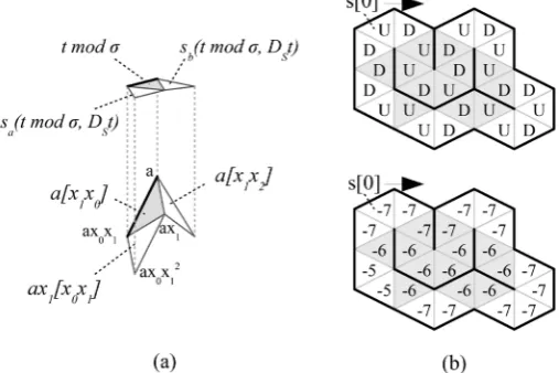
DOI: 10.4236/am.2019.1011065 921 Applied Mathematics Figure 4. Trajectory on B2. (a) A local trajectory associated with t a x x=

[

1 0

]

∈S2; (b)

The values of the U/D function (above) and the height function (below) on a closed trajectory shown in Figure 3(b). In the figure, U and D denotes +1 and −1, respectively. The trajectory starts from

[ ]

4 3

[

]

0 2 1 0

0 mod

s =x x x x σ and moves clockwise. For the boundary

edges e (thick line) of the grey triangles, the edge neighborhood N e

( )

is contained in the trajectory. Note that the boundary of the trajectory consists of the boundary edges of the white triangles. (See Proposition 2 and its Corollary.)

c

V is called a _3_-embeddable_{vector field of triangles. Note that} c

V has no singular triangle.

Remark 1. B2 =

{

tmod |σ t dc∈

}

, and the value of Vc is determined uni-quely on B2.

Example 9. Shown in Figure 3(c) and Figure 3(f) is the vector field Vc on 2

B induced by c Cone P P=

{

1, , ,2 P13

}

of Example 8.

Local trajectories of Vc on B2 (Definition 11) is computed as follows. Lemma 6. Let s B∈ 2. Let c L⊂ 3 be a tangent cone. Suppose that

( )

(

( )0 ( )1 mod 3

)

c S

V s =D a x x ρ ρ  σ . Then, the local trajectory of V sc

( )

at s is

either

( )

(

,

)

(

,

( )

)

a c b c

s s V s − −s s s V s

or

( )

(

,

)

(

,

( )

)

,

b c a c

s s V s − −s s s V s

where

( )

(

)

( ) ( ) ( )

( )

(

)

( ) ( )

0 1 0

0 2

, mod ,

, mod .

a c

b c

s s V s ax x x

s s V s a x x

ρ ρ ρ

ρ ρ

σ

 =  

  



 

=

 _ _

 Proof. See Lemma 4.

Lemma 7. Let s B∈ 2. Let c L⊂ 3 be a tangent cone. Let s0− −s s2 be the local trajectory of Vc at s. Then,

(

0 2

)

( )

.

t c

(16)

DOI: 10.4236/am.2019.1011065 922 Applied Mathematics Proof. Note that Vc has no singular triangle on B2. The result follows im-mediately.

Proposition 1. Let V be a vector field on B2 without singular triangles. Then,

3

a tangent cone c L such that V Vc.

∃ ⊂ =

Proof. See [4].

3.2.2. The U/D and Height Functions Associated with _3_-Embeddable

Vector Fields

Vector fields induced by a tangent cone are inherently associated with an U/D function and a height function.

Let s B∈ 2. Let c L⊂ 3 be a tangent cone. Suppose that

( )

(

_{( )} _{( )} 3

)

0 1 mod

c S

V s =D a x x_ ρ ρ _ σ . Then, the local trajectory at s is either a b

s − −s s _or s s s_b− − _a_{, where}

( ) ( )

( )

(

)

( ) ( ) ( )

( )

(

)

( ) ( )

0 1

0 1 0

0 2

mod ,

, mod ,

, mod

a a c

b b c

s a x x

s s s V s ax x x

s s s V s a x x

ρ ρ

ρ ρ ρ

ρ ρ

σ

 _{= } 

 

 ₌ ₌ _ _

 _ _



 

 = _{= } _

 (See Figure 4(a)).

Definition 23 (U/D function gS). Let s B∈ 2. Let c L⊂ 3 be a tangent cone. Let s

[ ] [ ] [ ]

0 −s1 −s 2 _{be the local trajectory of}V_c at s (i.e. s

[ ]

1 =s_{). The}_U_/_D

function gS at s along the trajectory associated with Vc is defined by

( )

, : 1, if 2

[ ]

_{[ ]}

1, if 2

a S

b

s s

g c s

s s

− =



= ₊ ₌



where sa and sb are given above. That is, −1 and +1 indicate “downhill” and “uphill” on the “mountain road” s

[ ] [ ] [ ]

0 −s1 −s 2 , respectively.

Remark 2. In Definition 14, U/D functions are not uniquely specified on an n-simplex space because the uphill and downhill along a trajectory are not given explicitly. On the other hand, the U/D function is uniquely specified on Bn us-ing the uphill and downhill along a trajectory of slant n-simplices.

_{( )}

_,

S

g c is an U/D function defined in Definition 14.

Proof. Let s

[ ] [ ] [ ]

0 −s1 −s 2 _{be a local trajectory of}V_c. Let

[ ]

1 ( )0 ( )1 mod

s = a x x ρ ρ  σ and V sc

( )

[ ]

1 =D a xS

(

 ρ( )0xρ( )1modσ3

)

. Suppose that g c sS

(

, 1

[ ]

)

= +1. Then, either

[ ]

(

2

)

(

1( )1 ( )1 ( )0 mod 3

)

c S

V s ₌D ax_ρ− _x x_ρ _ρ _ σ

 

or

[ ]

(

2

)

(

( )0 ( )2 mod 3

)

.

c S

V s ₌D a x _ρ x_ρ  σ

 

(17)

DOI: 10.4236/am.2019.1011065 923 Applied Mathematics where either

[ ]

( )

[ ]

(

)

(

2 , 1

)

(

( )0 ( )1 mod 3

)

c a c S

V s s V s =D a x x_ ρ ρ _ σ

or

[ ]

( )

[ ]

(

)

(

2 , 1

)

(

( )0 ( )2 ( )0 mod 3

)

,

c a c S

V s s V s =D axρ _xρ xρ _ σ

respectively. Since s

[ ]

1 = a x x ρ( )0 ρ( )1 _modσ , we obtain

[ ]

(

2

)

(

1( )1 ( )1 ( )0 mod 3

)

.

c S

V s =D axρ− x xρ ρ  σ

That is,

[ ]

(

)

(

[ ]

)

( )

[ ]

( )

[ ]

if g c sS , 2 =g c sS , 1 = +1, thenV sc 2 ∩V sc 1 = ∅.

Continuing in the same way for the other case, we obtain

[ ]

(

, 2

)

(

, 1 if and only if

[ ]

)

(

[ ]

2

)

( )

[ ]

1 .

S S c c

g c s =g c s V s ∩V s = ∅

Proposition 2. Let _{c L}_⊂ 3_{be a tangent cone. Let} _L₌

{

_{s k k I}

[ ]

_| _{∈ ⊂}_

}

_{be a} maximal trajectory of Vc on B2. Let s B∈ 2. Then,

( )

(c )

(

,

)

0 if

(

( )

)

.

S c

s N V s′∈ g c s N V s L

′ = ⊂

∑

Remark 3. The edge neighborhood N V s

(

c

( )

)

consists of two triangles which share the boundary edge V sc

( )

(Definition 4).

Proof. Let N V s

(

c

( )

)

=

{

s i s j

[ ] [ ]

,

}

(i< j). Suppose that

[ ]

(

,

)

(

,

[ ]

)

S S

g c s i =g c s j _{. Then, either}s i

[ ]

−1 _or s j

[

+1

]

_{is enclosed by the}

trajectory s i s i

[ ] [

− + − −2

]

s j

[ ]

of finite length, and the trajectory starting from the enclosed triangle (either s i

[ ] [

− −1 s i− −2

]

or

[

1

] [

2

]

s j+ −s j+ −) has an “end point”. However, Vc has no singular trian-gle, which is a contradiction.

Corollary 1. Suppose that L is closed. Then, the sum of g cS

( )

, over the

“boundary” of L is equal to zero, i.e.,

( )

, 0,

bd S s R∈ g c s

=

∑

where Rbd =

{

s L N V s∈ |

(

c

( )

)

⊂/L

}

.

Proof. Because of Proposition 2, the sum of g c_S

( )

, over L is equal to the sum of g cS

( )

, over the “boundary” of L, i.e.,

( )

,

( )

,

( )

,

( )

, ,

in bd bd

S S S S

s L∈ g c s s R∈ g c s s R∈ g c s s R∈ g c s

= + =

∑

where R_in =

{

s L N V s∈ |

(

_c

( )

)

⊂L

}

. Since the sum of g cS

( )

, over L is zero

when L is closed, the result follows.

Example 10. Shown in Figure 4(b) above is the value of the U/D function S

(18)

[ ]

(

)

(

[

]

)

[ ]

( )

(

[

]

)

[ ]

(

)

(

[

]

)

4 3 3

0 2 1 0

4 3 3

0 2 1 2

3 3 3

0 1 2 0 2

0 mod ,

1 mod ,

2 mod .

c S

V s D x x x x

V s D x x x x x

σ σ σ = = = Since

[ ]

(

[ ]

)

(

)

4 3

[

]

[ ]

0 2 1 2

0 , 0 mod 1 ,

b c

s s V s =x x x x σ =s

we obtain g c sS

(

, 0

[ ]

)

= +1. Since

[ ]

( )

[ ]

(

)

[

]

[

]

[ ]

4 3 0 1 2 2 1 3 3 0 1 2 0 2

1 , 1 mod

mod 2 ,

a c

s s V s x x x x x

x x x x x s σ σ = = =

we obtain g c sS

(

, 1

[ ]

)

= −1.

Note that two grey triangles sharing a thick edge have opposite values. The sum of the U/D function over the set of all the white triangles is equal to zero.

Definition 24 (Height function hS). The height function hS on L3 is a  -valued function defined by

(

0 1l m n2

)

:

(

)

. S

h x x x = − + +l m n

The heightfunction hS on S2 is a -valued function defined by

(

)

:

( )

.

S i j S

h a x x_  =_ h a

Let _{c L}_⊂ 3_{be a tangent cone. Then, the}_height _function S

h on B2 asso-ciated with Vc is a -valued function defined by

(

, mod

)

:

( )

.

S S

h c t σ =h t

where t dc∈ .

By an abuse of notation, we use the same name hS for three functions with different domains.

_{( )}

_,

S

h c is a height function with respect to g cS

( )

, defined in Definition 15.

Proof. Let s

[ ] [ ] [ ]

0 −s1 −s 2 _{be a local trajectory of}V_c. Then, h c_S

( )

, on

[ ]

2

s is given by

[ ]

(

, 2

)

(

₍

, 1

[ ]

_{[ ]}

)

₎

(

, 1 , if

[ ]

)

(

, 2

[ ]

)

(

, 1

[ ]

)

, 1 , otherwise

S S S S

S

h c s g c s g c s g c s

h c s

 + =

 =  

Proposition 3. Let s B∈ 2. Let c L⊂ 3 be a tangent cone. Then, h cS

( )

, is

constant on N V s

(

c

( )

)

=

{

s s0, 1

}

, i.e.,

(

, 0

)

(

, 1

)

.

S S

h c s =h c s

Proof. Since V sc

( )

0 =V sc

( )

1 , the result follows immediately.

Example 11. Shown in Figure 4(b) below is the value of the height function S

(19)

DOI: 10.4236/am.2019.1011065 925 Applied Mathematics triangles are

[ ]

(

)

(

[

]

)

[ ]

( )

(

[

]

)

[ ]

(

)

(

[

]

)

4 3 3

0 2 1 0

4 3 3

0 2 1 2

3 3 3

0 1 2 0 2

0 mod ,

1 mod ,

2 mod ,

c S

V s D x x x x

V s D x x x x x

σ σ

σ

=

where

x x x x

0 24 3

[ ]

1 0 ,

x x x x

0 24 3

[ ]

1 2 ,

x x x x x

30 1 23

[

0 2

]

∈

dc

. Then,

[ ]

(

)

(

4 3

[

]

)

( )

4 3 0 2 1 0 0 2

, 0 7.

S S S

h c s =h x x x x =h x x = −

In the same way, we obtain h c sS

(

, 1

[ ]

)

=h c sS

(

, 2

[ ]

)

= −7.

Note that two grey triangles sharing a thick edge have the same value.

3.2.3. _4_{-Embeddable Vector Fields of Tetrahedrons}

This paper proposes a novel mathematical approach for the design of self-assembling molecules, where self-assembling molecules are represented as a union of trajectories of tetrahedrons. Here we shall consider vector fields on a tetrahedron space which are induced by a four-dimensional tangent cone.

In the same way as for the space B2 of flat triangles, we shall define a “tetra-hedron space” by partitioning _E3_{into tetrahedrons of the same shape. “Three-} dimensional” vector fields of tetrahedrons then correspond to a “four-dimensional” drawing on the surface of “mountains” of unit cubes of _E4_.

Definition 25 (The four-dimensional lattice _L4_{). Let} _L4_{be the four-di-} mensional lattice generated by four vectors

(

1,0,0,0

)

,

(

0,1,0,0

)

,

(

0,0,1,0

)

, and

(

0,0,0,1

)

, i.e.,

{

}

4 4

0 1 2 3

: l m n k | , , , .

L = x x x x l m n k∈ ⊂E

Shown in Figure 5(a) is a unit cube of _L4_{and its “top view”.}

Definition 26 (The symmetric group _Sym4_{on four letters). Let} _Sym4_be the group of all the permutations of the set

{

0,1,2,3

}

. Elements of _Sym4_are written in cyclic notation. For example, let

_ρ

₌

( )

₀₂₁ _∈_Sym4_{. Then,} _ρ

_{( )}

₀ ₌₂_,

( )

1 0

ρ = , ρ

( )

2 1= , and ρ

( )

3 =3.

Definition 27 (The set B3 of all flat tetrahedrons). Let a L∈ 4 and ρ∈Sym4.

The slant tetrahedron a x x x ρ( ) ( ) ( )0 ρ1 ρ2 is defined by

( ) ( ) ( )0 1 2 : , ( )0, ( ) ( )0 1, ( ) ( ) ( )0 1 2 ,

a x x x ρ ρ ρ   = a axρ ax xρ ρ ax x xρ ρ ρ 

where

[

a b c d, , ,

]

denotes the convex hull of four points _{a b c d E}_{, , ,} _∈ 4 (Defi-nition 1).

Let S3 be the set of all slant tetrahedrons, i.e.,

( ) ( ) ( )

{

4 4

}

3: 0 1 2 | , .

S ₌ a x x x _ρ _ρ _ρ  a L_∈ ρ_∈Sym

 

The shiftoperator σ_on S₃ is defined by

( ) ( ) ( )

(

a x x xρ0 ρ1 ρ2

)

: axρ( )0 x xρ( )1 ρ( )2xρ( )3 .

σ _ _ = _ _

Then, an equivalence relation σ is defined on S3 by

( )

if and only if s.t. m .

a b a b

(20)

[image:20.595.261.484.70.317.2]

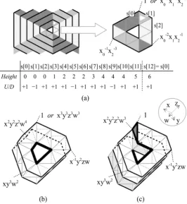
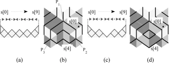
DOI: 10.4236/am.2019.1011065 926 Applied Mathematics Figure 5. Trajectory of tetrahedrons. (a) A unit cube of _L4_{represented by the Schlegel}

diagram (bottom) and its projection on a three-dimensional hypersurface (top); (b) A facet of a unit cube of _L4_{(bottom) and its projection on a three-dimensional hyper-}

surface (top), where Q1=1, Qx=x0, Qy=x1, Qz=x2, Qxz=x x0 2, Qxyz=x x x0 1 2, and

v

P is the projected image of Qv. The diagonal edge PP1 xyz is drawn with a thick line; (c) A tetrahedron and its six edges (thick lines). Edges are shown with the adjacent tetrahedrons associated with them. Only four of them (left and center) are included in the tangent space; (d) A chain of isosceles tetrahedrons consisting four short edges and two long edges (length ratio is 3 to 2), where tetrahedrons are connected via a long edge (left). By folding the chain of tetrahedrons, we shall obtain a trajectory of tetrahedrons (right). The boundary edges are drawn with thick lines; (e) Closed trajectories of the vector field on B3 induced by Cone P P P P

{

yzw, xzw, xyw, xyz

}

, where P_{x y z w}l m n k =x x x x0 1l m n k2 3 . The

boundary edges are drawn with thick lines.

The σ _{-equivalence class of}t S∈ ₃_{is called a}_flat _tetrahedron_{and denoted} by tmodσ_.

The set of all flat tetrahedrons is denoted by B3, i.e.,

3: 3 .

B =S σ

Example 12. The facet of a unit cube S3 shown in Figure 5(b) bottom con-sists of six slant tetrahedrons

[

] [