Eigenvalue analysis and case study examples of fractional order generalised predictive control

Eigenvalue Analysis and Case Study Examples of

Fractional Order Generalised Predictive Control

Y. Alarfaj and C. J. Taylor

Engineering Department, Lancaster University, UK Emails: [email protected], [email protected]

Abstract—This article concerns a previously developed, Fractional–order, Generalised Predictive Control (FGPC) ap-proach to control system design. Here, fractional order con-cepts are utilised to extend the design flexibility of the FGPC algorithm, in comparison to conventional Generalised Predictive Control (GPC). The performance of FGPC is investigated via Monte Carlo simulation. With a focus on plots of the closed-loop eigenvalues, these results are utilised to develop recommendations for how to optimise the extra design coefficients introduced in the fractional order case. One of the simulation examples involves a hydraulically actuated robotic manipulator. Finally, FGPC methods are applied to control airflow in a laboratory 1 m by 2 m by 2 m forced ventilation environmental test chamber.

Index Terms—generalised predictive control; fractional–order control; robotic manipulator; ventilation control

I. INTRODUCTION

This article concerns a Fractional–order, Generalised Pre-dictive Control (FGPC) design approach, as introduced by Romero et al. [1]–[4]. Although fractional order calculus has a long history in mathematics and engineering, the uptake of fractional order concepts for control system design and practical implementation has been slower than for equivalent integer order methods. Hence, the FGPC approach is of potential interest because of its relationship with the well-known, conventional control algorithm, Generalised Predictive Control (GPC) [5]–[7]. In fact, the algorithms take the same, relatively straightforward implementation form, making them potentially attractive to practitioners.

Fractional calculus can be defined as a generalization of derivatives and integrals to non-integer orders [8]. Fractional-order operators are commonly represented byαD, representing the α order derivative. Negative values of α correspond to fractional-order integrals, −α_{D ≡} α_{I. This operator can} be evaluated using the Grunwald-Letnikov definition for nu-merical integration and simulation purposes. To illustrate, one of the more active areas of research into fractional order control concerns Fractional order Proportional–Integral– Derivative (FPID) methods, with illustrative citations includ-ing [8]–[10]. Here, straightforward PID concepts, such as frequency domain analysis, are sometimes used to design higher order (once converted into an approximated form that can be implemented in practice) FPID control systems. These potentially yield improved performance in comparison to standard PID design. Further examples of fractional control include, for example, CRONE [11], fractional fuzzy adaptive control [12] and optimal control [13].

In general terms, the design task involves either integer-order or fractional-integer-order control systems, as applied to either integer-order or fractional-order models. Hence, for example, Allafi et al. [14] consider parameter estimation methods for fractional-order Hammerstein-Wiener models, using a Sim-plified Refined Instrumental Variable (SRIV) fractional-order continuous time algorithm. By contrast, the present article concerns the application of FGPC design to discrete-time, linear integer-order models. For the laboratory example, such models are estimated from data using the standard SRIV algorithm in the CAPTAIN toolbox for MATLAB [15].

Hence, the aim is to design FGPC systems that potentially yield improved performance over conventional GPC design. The FGPC methodology is briefly reviewed (section II), and a worked example using MATLAB is developed to illustrate the FGPC design approach (section III). Further simulation examples are utilised to demonstrate how fractional order methods increase the control design flexibility compared to GPC. In contrast to references [1]–[4], the influence of the new FGPC tuning coefficients, α and β, are systematically investigated via Monte Carlo simulation. The focus is on cloud plots of the closed-loop eigenvalues (poles). The study is ex-tended to a laboratory example, namely the control of airflow in a 1 m by 2 m by 2 m forced ventilation environmental test chamber (section IV). Discussion and conclusions follow (sections V and VI).

II. METHODOLOGY

Similar to conventional discrete-time GPC, FGPC is based on the following Auto–Regressive, Integrated Moving– Average eXogenous variables (ARIMAX) model, sometimes also called a Controlled Auto–Regressive Integrated Moving– Average (CARIMA) model,

y(k) =B(z −1₎

A(z−1₎u(k) +

T(z−1)

∆A(z−1₎ζ(k) (1)

or equivalently

∆A(z−1)y(k) =B(z−1)∆u(k) +T(z−1)ζ(k) (2)

wherey(k)is the output at samplek,u(k)is the control input,

ζ(k) is uncorrelated white noise and ∆ = 1−z−1 is the difference operator, in which z−1 _{is the backward operator,} i.e. z−1_{y(k) = y(k−1). Finally, A(z}−1_{) = 1 +a}

1z−1+

m andq respectively. Finally, pure time–delays ofδ samples are straightforwardly represented by setting the leadingδ−1 coefficients ofB(z−1)to zero, i.e.b1=b2=· · ·=bδ−1= 0.

A. Standard GPC

Standard GPC is based on the following cost function,

JGPC(∆u, k) =

N2 X

i=N1

γie(k+i)2+ Nu

X

i=1

λi∆u(k+i)2 (3)

where e(k) = r(k+i)−y(k+i), in which r(k) is the set point,N1 andN2are forecasting horizons associated with the output variable, andNuis the input forecasting horizon. When minimizing (3), it is assumed that u(k) is time-invariant for

k > Nu, whereN1 ≤Nu≤N2. The simplest form of GPC also assumes a time-invariant set point in equation (3), and is based on the model (1) with the noise polynomial fixed as unity, i.e. T(z−1) = 1. Finally, γi and λi are non-negative weighting elements.

The weights are sometimes expressed in matrix form as follows: Γ =diag(γi) andΛ =diag(λi). In fact, for many practical applications, it is further assumed that N1 = 1,

Γ = I and Λ = diag(λ), where I is the identity matrix and λ is a scalar weight on the input variable. This yields a GPC algorithm that is straightforward to tune (often by trial and error) for practical applications using just three terms i.e.

N2,NU andλ(somewhat analogous to a classical three term industrial PID controller).

The present article concerns linear controllers that can be analysed in block diagram terms, hence no constraints are defined for the input and output variables. Minimising the cost function (3) under all the above assumptions yields a fixed gain control algorithm that can be conveniently expressed in polynomial form as follows (see e.g. [5]–[7], [16]),

∆u(k) = 1

R0_(z−1₎ w0r(k)−S

0_(z−1_)y(k)

(4)

where,

S0(z−1) = s00+s10z−1+· · ·+s0nz−n (5)

R0(z−1) = 1 +r0₁z−1+· · ·+r0_m−1z−m+1 (6) and w0 is a command input gain. Alternatively, defining

S(z−1) =S0(z−1)/w0 andR(z−1) =R0(z−1)/w0 yields,

∆u(k) = 1

R(z−1₎ r(k)−S(z

−1_)y(k)

(7)

where,

S(z−1) = s0+s1z−1+· · ·+snz−n (8)

R(z−1) = r0+r1z−1+· · ·+rm−1z−m+1 (9) Substituting (7) into the deterministic component of equa-tion (1) yields the following closed–loop Transfer Funcequa-tion,

y(k) = B(z

−1₎

∆R(z−1_)A(z−1_{) +S(z}−1_)B(z−1₎r(k) (10)

The closed–loop poles pi are determined from the character-istic equation:∆R(z−1)A(z−1) +S(z−1)B(z−1) = 0.

B. Fractional order GPC

Initially posed in continuous-time terms, so as to allude to selected concepts in fractional calculus, Romeroet al.[1]–[4] define the following cost function for FGPC design,

JFGPC(∆u, t) =αI

N2

N1(r(t)−y(t)) 2

+βINu

1 (∆u(t)) 2

(11)

where I is the fractional-order definite integral operator, and α, β ∈ _R are user defined coefficients representing the fractional order. The operator I and hence equation (11) is subsequently discretized as shown by the references cited above. Minimisation of the associated discrete–time cost func-tion yields a controller with the same structural form as GPC, i.e. it is defined by equations (7)–(9). The main difference is that, whilst the GPC weighting matricesΓ andΛare defined explicitly via the cost function (3), or more commonly in practice via the scalar input weight λ as described above, FGPC defines these weights implicitly via the two scalar tuning terms, αandβ.

III. SIMULATIONSTUDY

Romero et al. [1] define three types of GPC or FGPC design. This is illustrated by their numerical example, which is reproduced in the first case study example below.

A. Worked example

Consider a first order, non-minimum phase model based on equation (1), withT(z−1) = 1,

y(k) =z

−1_−2z−2

1−0.9−1 u(k) +ζ(k) (12) For illustrative purposes, arbitrarily define N1 = 1, N2 = 10, Nu = 2 andλ= 10−6 i.e. the GPC weighting matrices are Γ = I10 and Λ = 10−6 I2. Minimising the GPC cost function (3) yields equations (7)–(9) with s0= 3.9539,s1=

−2.9539, r0 =−1.7892 andr1 =−6.5642. The associated closed–loop poles are p1 = p2 = 0 and p3 = 0.4411. The input and output responses to a unit step in the set point are shown in Fig. 1 (i.e. the traces labelled GPC in the legend).

UtilisingN1= 1,N2= 10andNu= 2 as above, together with α=β = 2.5, FGPC design yields s0 = 4.2999,s1 =

−3.2999,r0=−2.2982andr1=−7.3331. The closed–loop poles are p1 = 0, p2 = 0.0277 and p3 = 0.5525, with the response shown as the dashed black traces in Fig. 1. This response is labelled FPGC–2 on the legend, since Romero et al. [1] define this as an example of Type 2 FGPC control.

In fact, conventional GPC design can be utilised to de-termine identical control gains as for Type 2 FGPC. This is achieved by appropriate bespoke choice of Γ and Λ. For this example, the relevant diagonal elements of Γare: 23.67, 21.14, 17.81, 14.66, 11.73, 9.02, 6.56, 4.38, 2.5, and 1.0; and the diagonal elements ofΛ are: 1.5 and 1.0. In other words, for this example, α = β = 2.5 represent high level tuning parameters (hyper-parameters) that determine the Γ and Λ

weighting matrices.

Fig. 1. Closed-loop response of the model (12) to a unit step in the set point for GPC, FGPC with α = 1.2and β = 0.8(FGPC–3), and FGPC with α=β= 2.5(FGPC–2). Upper plot: outputy(k)against sample numberk. Lower: control inputu(k). Based on reference [1].

using the FGPC tuning approach, they call it Type 2, other-wise it is Type 1. Finally, Type 3 control is obtained when

α < 1 or β < 1 in FGPC design. In the latter case, the weighting sequences can include negative terms in Γ and/or

Λ respectively. For example, solving the FGPC cost (11) for

α = 1.2 and β = 0.8 yields diagonal elements of Γ: 0.71, 1.68, 1.63, 1.59, 1.54, 1.48, 1.41, 1.32, 1.2 and 1.0; and diagonal elements of Λ: −0.2 and 1.0. Here, FGPC design yields equations (7)–(9) with s0 = 3.7146, s1 = −2.7146,

r0=−1.4264andr1 =−6.0325. The closed–loop poles are

p1= 0,p2=−0.0695andp3= 0.3445, with the response to a unit step in the set point shown in Fig. 1 (labelled FGPC–3). Note that one of the input weights is a negative number and also that a closed–loop pole appears on the left hand side of the complexz–plane.

B. Eigenvalues

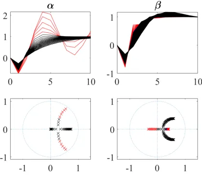
Continuing with the model (12), Fig. 2, Fig. 3 and Fig. 4 investigate how the control tuning coefficients determine the closed-loop pole positions (eigenvalues) and hence the time response. With N1 = 1, N2 = 10 and Nu = 2, the left hand side subplots of Fig. 2 show the output responses (upper subplot) and the eigenvalues (lower subplot), when α

is varied in the range 0 → 5. For α <≈ 1.6, a complex conjugate pair of poles appears, with the complex component gradually increasing as αis decreased further. The associated poorly damped, oscillatory responses are particularly evident forα <1, for which the responses and eigenvalues are shown in red colour in Fig. 2. In a similar manner, the right hand side subplots of Fig. 2 considerβvaried in the range0→10. Here, with β < 1, for which the responses and eigenvalues are again plotted in red colour, one of the eigenvalues moves into the left hand side of the complex z–plane.

Fig. 2. Closed-loop FGPC responses of the model (12) to a unit step in the set point withN2 = 10andNu= 2. Left hand side plots:β = 2.5and

α= [0 : 0.2 : 5]. Right hand side plots:α= 1.2andβ= [0 : 0.1 : 10]. Upper plots:y(k)againstk. Lower plots: eigenvalues shown on the complex z–plane. Red colour shows the case withαorβ <1, otherwise black.

Fig. 3 represents a systematic variation of both α and β

across the same range of values (right hand side subplots). For comparison, the left hand side subplots consider GPC withλin the range 10−7→107. Here, it is clear that many combinations of αandβ yield an unsatisfactory closed–loop response, especially when either α or β are less than unity i.e. Romero et al. [1] Type 3 control. Nonetheless, Fig. 3 demonstrates how FGPC can be used to extend the range of closed-loop realisations that are possible and, in principle, some of these realisations might represent a controller that meets a defined set of control objectives (e.g. for performance and robustness).

Finally, Fig. 4 illustrates this result in more general terms (albeit limited to the same model). Here, the various tuning coefficients considered in this article (N2,Nu,λ,αandβ) are all varied simultaneously, to show how FGPC potentially cap-tures more of the complexz–plane than the more constrained GPC approach. However, whether or not the increased range of eigenvalues facilitates a better control algorithm for a given practical application requires further research. Indeed, it is well understood from the literature on GPC that straightforward tuning ofN2,Nuandλalready yields a satisfactory design for many applications. By contrast, inadvisable choice ofαandβ

can clearly yield a highly unsatisfactory and even unstable FGPC design. To illustrate, the left hand side eigenvalues in Fig. 4 are typically associated with an oscillatory closed-loop response (for brevity, these time-responses are omitted).

C. Marginally stable system

Fig. 3. Closed-loop GPC (left) and FGPC (right) responses of the model (12) to a unit step in the set point with N2 = 10and Nu = 2. Left hand

side plots: GPC withλ = 10[−7:0.2:7]_{. Right hand side plots: FGPC with}

α= [0 : 0.2 : 5]andβ = [0 : 0.1 : 10](all possible realisations). Upper plots:y(k)againstk. Lower plots: eigenvalues shown on the complex z– plane. Red colour shows the case withαorβ <1, otherwise black.

Fig. 4. Closed-loop GPC (left) and FGPC (right) eigenvalues shown on the complex z–plane, for 10000 random realisations of the tuning coefficients from the following uniformly distributed ranges:N2= [3 : 20],Nu= [1 :

N2−1],λ= 10[−7:7],β= [0 : 10]andα= [0 : 10]. Red colour shows

the case withαorβ <1, otherwise black.

authors including e.g. [15] (p. 70).

y(k) = −z

−2_{+ 2z}−3

1−1.7z−1_+z−2u(k) (13) Fig. 5 shows the eigenvalues and time-responses of the model (13) for a range of values of λ(GPC) andβ (FGPC). The envelope of time responses for GPC and FGPC cover a similar range, whilst the main difference for FGPC is that one of the closed–loop poles moves along the real axis of the complex z–plane (close to but not at the origin). The authors are presently investigating if these poles can provide any improvements over GPC in terms of robustness for this marginally stable system, and these results will be reported in future articles.

D. Robotic manipulator

This simulation example is based on a robotic system in the laboratory. The hardware configuration consists of two off–the–shelf HydroLek 7W manipulators, whose joints are

Fig. 5. Closed-loop GPC (left) and FGPC (right) responses of the model (13) to a unit step in the set point withN2= 10andNu= 9. Left hand side plots:

GPC withλ= 10[−3:0.1:4]_{. Right hand side plots: FGPC withα= 2.5and}

β= [0 : 0.17 : 12]. Upper plots:y(k)againstk. Lower plots: eigenvalues shown on the complex z–plane. Red colour shows the case with β < 1, otherwise black.

controlled using potentiometer sensors and hydraulic actuators, and a Brokk 40 mobile platform used to support and transport the device. Each 6–degree–of–freedom manipulator has a con-tinuous jaw rotation mechanism and dual function gripper fit-ted with a pressure sensor. The movements of the manipulator joints are controlled through hardware and software integration using LabviewR and associated National Instruments tools.

Such dual–arm mobile robots offer a powerful option for nuclear decommissioning applications [17]–[19].

Dynamic cross–coupling affects for the various HydroLek joints are usually relatively small, hence to illustrate the single-input, single-output control approach developed in section II, the present analysis focuses on an illustrative joint considered in isolation. In this regard, open–loop step experiments suggest that a first order linear differential equation provides an ap-proximate representation of individual joints. In fact, using an arbitrary (for illustrative purposes) calibration framework for the wrist joint of the left hand side manipulator, equation (1) with n = 1, m = 2, δ = 2, a1 = −1, b1 = 0.1 and

T(z−1) = 1provides a suitable model for initial linear control system design [17]. Here,y(k)represents the joint angle and

u(k)is a scaled voltage in the range±10, where positive and negative signs are used to indicate clockwise or anticlockwise movement. Fig. 6 shows the simulated closed–loop response of an illustrative FGPC design withN1= 1,N2= 10,Nu= 2,

α = 2.5 and β = 2.5. Here, an output step disturbance of magnitude 0.2 is simulated from the 22nd sample onwards, representing an applied load to the system.

Fig. 6. Simulated FGPC control of robotic manipulator joint angle with a disturbance at samplek= 22, showing the output (upper subplot) and control input (lower) plotted against sample number.

IV. LABORATORYEXAMPLE

Previous research has considered a laboratory forced venti-lation chamber with an array of 30 thermocouples distributed within a 2 m ×1 m ×2 m airspace, with airflow sensors at the inlet and outlet [22]. Actuators include two axial fans and a 400 W heating element, used to generate various micro-climatic conditions for research into buildings environment control. The operation of the chamber is controlled by National Instruments hardware/software.

Fig. 7 considers control of airflow at the outlet y(k)(m/s), using the applied voltage to the outlet fan as the control input u(k) i.e. an analogue 0 → 5 V DC output from the National Instruments card inside the control computer. Here, the linearised model for an operating condition of 2.25 m/s is based on equation (1) with a1 = −0.8470, b2 = 0.5325 and δ = 2, identified from open–loop data using the RIV algorithm of the CAPTAIN Toolbox [15]. Straightforward trial and error FGPC tuning using this control model in simulation mode yields a satisfactory response with N1 = 1,N2 = 20,

Nu = 5, α= 0.5 and β = 2.2, as illustrated in Fig. 7. On-going research by the first author is considering the relative robustness and performance of the FGPCP algorithm in com-parison to GPC. Nonetheless, the present results represent one of the first practical implementations of the FGPC approach.

V. DISCUSSION

In general terms, model-based design (e.g. pole placement, GPC, FGPC) provides a quantitative method to determine the gains of the control system, based on the ‘desired’ performance of the closed-loop system. For the pole assignment method, performance relates to the poles of the closed-loop system, for GPC it is the minimisation of the cost function (3) and for FGPC it is the minimisation of (11). The latter cost function includes two scalar hyper-parameters,αandβ, and the impact of these parameters has been investigated in this article. Of

Fig. 7. FGPC control of ventilation rate in environmental test chamber, comparing the simulated (thick traces) and experimental (thin) data. Upper subplot: output air velocityy(k)(m/s). Lower subplot: control inputu(k)

(applied voltage in the range0→5V).

course, various different model-based design approaches can all produce the same outcome if the design criteria are set ‘correctly’ [23].

For example, conventional pole assignment can be utilised to set the closed-loop poles corresponding to the poles that minimise the GPC or FGPC cost (once these are known). Hence, it can be argued that the choice ofαandβis somewhat arbitrary. Indeed, Romeroet al. [1]–[4] provide no academic justification for why a fractional order cost function should be used nor any physically-based (engineering) reasons for how to selectαandβ, with trial and error via simulation being the implicit suggestion, as used in the present work.

Within the context of the assumptions made above, FGPC provides a generalisation of the GPC cost function weights, which ultimately determines the numerical values of the control gains in equations (8) and (9). Hence, the value of the approach appears dependent on whether the extra design flexibility provided by FGPC can be utilised to meet control objectives that are not achievable using standard GPC; and whether FGPC provides a straightforward to tune control algorithm – for example, that the use of α and β in this way provides a meaningful or convenient approach to solve practical control problems.

The first of these issues was considered by the simulation study in section III. The numerical results in this article show that the new tuning coefficientsαand β can indeed be used to potentially ‘capture’ more of the complex z–plane (with the closed-loop eigenvalues) than the more constrained GPC approach. However, whether or not the increased range of eigenvalues, and hence potential time responses and other closed–loop characteristics, could facilitate a better control algorithm (e.g. for a given practical application and set of control objectives) requires further research.

regard to the control of airflow in a forced ventilation chamber. In this case, straightforward trial and error FGPC tuning yields a satisfactory response for this laboratory system. However, it would be true to say that the same applies to conventional GPC design, pole assignment [15] and various other model-based approaches [22]. Hence, on-going research by the first author is considering the relative robustness and performance of the FGPC algorithm in comparison to GPC.

One limitation of the present work is that whilstαis used in FGPC design to provide a weighting on the output in the cost function (11), it has been assumed above that γ in the GPC cost (3) is unity throughout, as is common in many practical applications. It has also been assumed thatλi=λ(∀i)for the GPC simulations in this article. Hence, on-going research by the present first author concerns a comparison of FGPC and GPC without these constraints.

VI. CONCLUSIONS

This article has used both numerical examples and a lab-oratory test rig to investigate FGPC methods for control system design. The simulation study shows how FGPC can be used to extend the design flexibility of the conventional GPC algorithm. However, the value of these results in respect to control system robustness and performance, in both theoretical and practical terms, requires further research. Nonetheless, the method was applied to control airflow in a laboratory forced ventilation test chamber, representing one of the first practical implementations of FGPC design.

In further research, the authors are looking into other appli-cations and the relationship with recent research into predictive control using fractional order concepts. For example, Zou et al. [24] apply fractional order predictive functional control to industrial processes, whilst Shi et al. [25] apply fuzzy generalised predictive control to a fractional-order nonlinear hydro-turbine regulating system.

ACKNOWLEDGMENTS

This work is supported by the UK Engineering and Physical Sciences Research Council (EPSRC), grant EP/R02572X/1.

REFERENCES

[1] M. Romero, A. de Madrid, C. Manoso, and B. Vinagre, “Fractional-order generalized predictive control: Formulation and some properties,” in11th International Conference on Control, Automation, Robotics and Vision, Singapore, 2010.

[2] M. Romero, A. de Madrid, C. Manoso, and R. Hern´andez, “Generalized predictive control of arbitrary real order,” inNew trends in nanotechnol-ogy and fractional calculus applications. Springer, Dordrecht, 2010. [3] M. Romero, A. de Madrid, C. Manoso, and B. Vinagre, “A survey of

fractional-order generalized predictive control,” in51st IEEE Conference on Decision and Control, Maui, Hawaii, USA, 2012.

[4] M. Romero, A. de Madrid, C. Manoso, V. Milanes, and B. Vinagre, “Fractional-order generalized predictive control: Application for low-speed control of gasoline-propelled cars,” Mathematical Problems in Engineering, 2013.

[5] D. W. Clarke, C. Mohtadi, and P. S. Tuffs, “Generalized predictive control,”Automatica, vol. 23, pp. 137–148, 1987.

[6] D. W. Clarke, Ed., Advances in Model–Based Predictive Control. Oxford University Press, Oxford, 1994.

[7] R. R. Bitmead, M. Gevers, and V. Wertz, Adaptive Optimal Control: The Thinking Man’s GPC. Prentice Hall, 1990.

[8] I. Podlubny,Fractional Differential Equations. Academic Press, San Diego, 1999.

[9] F. Merrikh-Bayat, N. Mirebrahimi, and M. Khalili, “Discrete-time fractional-order PID controller: Definition, tuning, digital realization and some applications,”International Journal of Control, Automation, and Systems, vol. 13, no. 1, pp. 81–90, 2015.

[10] A. Lopes and J. Tenreiro Machado, “Discrete-time generalized mean fractional order controllers,” IFAC PapersOnLine, vol. 51, no. 4, pp. 43–47, 2018.

[11] A. Oustaloup, X. Moreau, and M. Nouillant, “The crone sustension,” Control Engineering Practice, vol. 4, pp. 1101–1108, 1996.

[12] E. Mehmet, “Fractional fuzzy adaptive sliding–mode control of a 2– DOF direct drive robot arm,”IEEE Transactions on Systems, Man, and Cybernetics, vol. 8, pp. 1561–1570, 2008.

[13] A. Oustaloup, X. Moreau, and M. Nouillant, “Optimal observer-based feedback control for linear fractional-order systems with periodic co-efficients,”Journal of Vibration and Control, vol. 25, pp. 1379–1392, 2019.

[14] W. Allafi, I. Zajic, K. Uddin, and K. Burnham, “Parameter estimation of the fractional-order Hammerstein-Wiener model using simplified refined instrumental variable fractional-order continuous time,” IET Control Theory and Applications, vol. 11, pp. 2591–2598, 2017.

[15] C. J. Taylor, P. C. Young, and A. Chotai,True Digital Control: Statistical Modelling and Non–Minimal State Space Design. John Wiley and Sons, 2013.

[16] C. J. Taylor, A. Chotai, and P. C. Young, “State space control system design based on non–minimal state–variable feedback: further generali-sation and unification results,”International Journal of Control, vol. 73, no. 14, pp. 1329–1345, 2000.

[17] C. J. Taylor and D. Robertson, “State–dependent control of a hydraulically–actuated nuclear decommissioning robot,”Control Engi-neering Practice, vol. 21, no. 12, pp. 1716–1725, 2013.

[18] T. Burrell, C. West, S. Monk, A. Montazeri, and C. J. Taylor, “Towards a cooperative robotic system for autonomous pipe cutting in nuclear de-commissioning,” inUKACC 12th International Conference on Control, Sheffield, UK, September 2018.

[19] M. Bandala, C. West, S. Monk, A. Montazeri, and C. J. Taylor, “Vision– based assisted tele–operation of a dual–arm hydraulically actuated robot for pipe cutting and grasping in nuclear environments,”Robotics, vol. 8, no. 6: 42, pp. 1–24, 2019.

[20] Y. Wang, L. Gu, Y. Xu, and X. Cao, “Practical tracking control of robot manipulators with continuous fractional-order nonsingular termi-nal sliding mode,”IEEE Transactions on Industrial Electronics, vol. 63, pp. 6194–6204, 2016.

[21] N. Nikdel, M. Badamchizadeh, V. Azimirad, and M. Ali Nazari, “Fractional-order adaptive backstepping control of robotic manipulators in the presence of model uncertainties and external disturbances,”IEEE Transactions on Industrial Electronics, vol. 63, pp. 6249–6256, 2016. [22] I. Tsitsimpelis and C. J. Taylor, “Partitioning of indoor airspace for

multi–zone thermal modelling using hierarchical cluster analysis,” in 14th European Control Conference, Linz, Austria, July 2015. [23] E. D. Wilson, Q. Clairon, R. Henderson, and C. J. Taylor,

“Ro-bustness evaluation and robust design for proportional—integral-–plus control,” International Journal of Control, 2018 (In press, https://doi.org/10.1080/00207179.2018.1467042).

[24] Q. Zou, Q. Jin, and R. Zhang, “Design of fractional order predictive functional control for fractional industrial processes,”Chemometrics and Intelligent Laboratory Systems, vol. 152, pp. 34–41, 2016.