http://www.scirp.org/journal/ajor ISSN Online: 2160-8849
ISSN Print: 2160-8830
DOI: 10.4236/ajor.2018.82009 Mar. 30, 2018 112 American Journal of Operations Research
The Sliding Gradient Algorithm
for Linear Programming
Hochung Lui, Peizhuang Wang
College of Intelligence Engineering and Mathematics, Liaoning Technical University, Fuxin, China
Abstract
The existence of strongly polynomial algorithm for linear programming (LP) has been widely sought after for decades. Recently, a new approach called Gravity Sliding algorithm [1] has emerged. It is a gradient descending method whereby the descending trajectory slides along the inner surfaces of a polyhe-dron until it reaches the optimal point. In R3, a water droplet pulled by
gravi-tational force traces the shortest path to descend to the lowest point. As the Gravity Sliding algorithm emulates the water droplet trajectory, it exhibits strongly polynomial behavior in R3. We believe that it could be a strongly
po-lynomial algorithm for linear programming in Rn too. In fact, our algorithm
can solve the Klee-Minty deformed cube problem in only two iterations, ir-respective of the dimension of the cube. The core of gravity sliding algorithm is how to calculate the projection of the gravity vector g onto the intersection of a group of facets, which is disclosed in the same paper [1]. In this paper, we introduce a more efficient method to compute the gradient projections on complementary facets, and rename it the Sliding Gradient algorithm under the new projection calculation.
Keywords
Linear Programming, Mathematical Programming, Complexity Theory, Optimization
1. Introduction
The simplex method developed by Dantiz [2] has been widely used to solve many large-scale optimizing problems with linear constraints. Its practical per-formance has been good and researchers have found that the expected number of iterations exhibits polynomial complexity under certain conditions [3] [4] [5] [6]. However, Klee and Minty in 1972 gave a counter example showing that its
How to cite this paper: Lui, H.C. and Wang, P.Z. (2018) The Sliding Gradient Algorithm for Linear Programming. Ameri-can Journal of Operations Research, 8, 112-131.
https://doi.org/10.4236/ajor.2018.82009
Received: February 26, 2018 Accepted: March 27, 2018 Published: March 30, 2018
Copyright © 2018 by authors and Scientific Research Publishing Inc. This work is licensed under the Creative Commons Attribution International License (CC BY 4.0).
http://creativecommons.org/licenses/by/4.0/
DOI: 10.4236/ajor.2018.82009 113 American Journal of Operations Research worst case performance is
( )
2n [7]. Their example is a deliberately con-structed deformed cube that exploits a weakness of the original simplex pivot rule, which is sensitive to scaling [8]. It is found that, by using a different pivot rule, the Klee-Minty deformed cube can be solved in one iteration. But for all known pivot rules, one can construct a different deformed cube that requires exponential number of iterations to solve [9] [10] [11]. Recently, the interior point method [12] has been gaining popularity as an efficient and practical LP solver. However, it was also found that such method may also exhibit similar worse case performance by adding a large set of redundant inequalities to the Klee-Minty cube [13].Is it possible to develop a strongly polynomial algorithm to solve the linear programming problem, where the number of iterations is a polynomial function of only the number of constraints and the number of variables? The work by Barasz and Vempala shed some light in this aspect. Their AFFINE algorithm [14] takes only
( )
2n
iterations to solve a broad class of deformed products de-fined by Amenta and Ziegler [15] which includes the Klee-Minty cube and many of its variants.
In certain aspect, the Gravity Sliding algorithm [1] is similar to the AFFINE algorithm as it also passes through the interior of the feasible region. The main difference is in the calculation of the next descending vector. In the gravity fall-ing approach, a gravity vector is first defined (see Section 3.1 for details). This is the principle gradient descending direction where other descending directions are derived from it. In each iteration, the algorithm first computes the descend-ing direction, then it descends from this direction until it hits one or more facets that forms the boundary of the feasible region. In order not to penetrate the feasible region, the descending direction needs to be changed. The trajectory is likened a water droplet falling from the sky but is blocked by linear planar structures (e.g. the roof top structure of a building) and needs to slide along the structure. The core of gravity sliding algorithm is how to calculate the projection of the gravity vector g onto the intersection of a group of facets. This projection vector lies on the intersection of the facets and hence lies on the null space de-fined by these facets. Conventional approach is to compute the null space first and then find the projection of g onto this null space. An alternative approach is disclosed in [1] which operates directly from the subspace formed by the inter-secting facets. This direct approach is more suitable to the Gravity Sliding algo-rithm. In this paper, we further present an efficient method to compute the gra-dient projections on complementary facets and also introduce the notion of se-lecting the steepest descend projection among a set of candidates. With these re-finements, we rename the Gravity Sliding algorithm as the Sliding Gradient al-gorithm. We have implemented our algorithm and tested it on the Klee-Minty cube. We observe that it can solve the Klee-Minty deformed cube problem in only two iterations, irrespective of the dimension of the cube.
DOI: 10.4236/ajor.2018.82009 114 American Journal of Operations Research Cone-Cutting Theory [16], which is the intuitive background of the Gravity Sliding algorithm. Section 3 discusses the Sliding Gradient algorithm in details. The pseudo-code of this algorithm is summarized in Section 4 and Section 5 gives a walk-through of this algorithm using the Klee-Minty as an example. This section also discusses the practical implementation issues. Finally, Section 6 dis-cuss about future work.
2. Cone-Cutting Principle
The cone-cutting theory [16] offers a geometric interpretation of a set of inequa-lity equations. Instead of considering the full set constraint equations in a LP problem, the cone-cutting theory enables us to consider a subset of equations, and how an additional constraint will shape the feasible region. The geometric insight forms the basis of our algorithm development.
2.1. Cone-Cutting Principle
In an m-dimension space m , a hyperplane T
c
=
y
τ
cuts m into two half spaces. Here τ is the normal vector of the hyperplane and c is a constant. We
denote the positive half space
{
T}
| ≥cy y τ the accepted zone of the hyperplane and the negative half space where
{
y y| Tτ<c}
is rejected zone. Note that the normal vector τ points to accepted zone area and we call the hyperplane withsuch orientation a facet
α τ
:
( )
,
c
. When there are m facets in m and{
τ τ
1, ,
2
,
τ
m}
are linear independent, this set of linear equations has a unique solution which is a point V in m. Geometrically,{
}
1
,
2,
,
mα α
α
form a cone and V is the vertex of the cone. We now give a formal definition of a cone, which is taken from [1].Definition 1. Given m hyperplanes in m, with rank
(
)
1
,
,
mr
α
α =
m
and intersection V,C
=
C
(
V
;
α
1,
,
α
m)
=
α
1
α
m is called a cone inm
. The
area
{
T(
)
}
| i ≥c ii =1, 2, ,m
y yτ is called the accepted zone of C. The point V is the vertex and αj is the facet plane, or simply the facet of C.
A cone C also has m edge lines. They are formed by the intersection of (m − 1) facets. Hence, a cone can also be defined as follows.
Definition 2. Given m rays Rj=
{
V+trj| 0≤ < +∞t}
(
j=1,,m)
shootingfrom a point V with rank
r
(
r
1,
,
r
m)
=
m
,C
=
C
(
V r
; ,
1
,
r
m)
=
c R
[
1,
,
R
m]
,the convex closure of m rays is called a cone in m
. Rj is the edge, rj the edge direction, and Rj+=
{
V+trj|∞ < < +∞t}
the edge line of the cone C.The two definitions are equivalent. Furthermore, P.Z. Wang [11] has observed that
R
i+ and
i
α are opposite to each other for i=1,,m. Edge-line
R
i+ isthe intersection of all C-facets except αi, while facet αi is bounded by all
C-edges except
R
i+ . This is the duality between facets and edges. For
{
}
1,
, ,
i,
ii
=
m
τ
R
is called a pair of cone C. It is obvious that T0
j i=
r
τ
(for i≠ j) since rj lies on αi. Moreover, wehave
(
)
T
0 for 1, ,
i i≥ i= m
r
τ
DOI: 10.4236/ajor.2018.82009 115 American Journal of Operations Research
2.2. Cone Cutting Algorithm
Consider a linear programming (LP) problem and its dual: (Primary): max
{
c xT |Ax≤b x; ≥0}
(2)
(Dual):
{
T T}
min y b y| A≥c;y≥0
(3) In the following, we focus on solving the dual LP problem. The standard simplex tableau can be obtained by appending an m m× identity matrix Im m× which represents the slack variables as shown below:
11 1 1
1
1
1 0
0 1
0 0 0
n
m mn m
n
a a b
a a b
c c
…
We can construct a facet tableau whereby each column is a facet denoted as
(
)
: , j j cj
α τ , where
(
)
T1, 2, ,
i = a ai i ami
τ and
for 1 0 for
i i
c i n
c
n i m n
≤ ≤
= < ≤ +
(4) The facet tableau is depicted as follow. The last column
(
)
T1, 2, , m, 0
b b b is
not represented in this tableau.
1 2
1 2
1 2
m n
m n
m n
c c c
α α α +
+
+
τ τ τ
When a cone
C
=
C
(
V
;
α
1,
,
α
m)
=
C
(
V r
; ,
1
,
r
m)
is intersected by anotherfacet αj, the i
th edge of the cone is intersected by
j
α at certain point qij. We call αj cuts the cone C and the cut points qij can be obtained by the following equations:
(
T)
Twhere
ij= +ti i ti = ci− j i j
q V r V τ r τ
(5) The intersection is called real if ti≥0 and fictitious if ti<0. Cone cutting
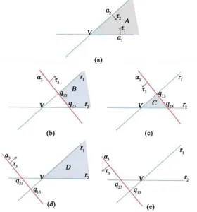
greatly alters the accepted zone, as can be seen from the simple 2-dimension example as shown in Figures 1(a)-(e). In 2-dimension, a facet
α τ
:
( )
,
c
is a line. The normal vector τ is perpendicular to this line and points to theac-cepted zone of this facet. Furthermore, a cone is formed by two non-parallel fa-cets in 2-dimension. Figure 1(a) shows such a cone
C
(
V
;
α α
1,
2)
. The acceptedzone of the cone is the intersection of the two accepted zones of facets α1 and α2.
This is represented by the shaded area A in Figure 1(a). In Figure 1(b), a new facet α3 intersects the cone at two cut points q13 and q23. They are both real
cut points. Since the arrow of normal vector τ3 points to the same general
di-rection of the cone, V lies in the rejected zone of α3 and we say α3 rejects V.
Moreover, the accepted zone of α3 intersects with the accepted zone of the cone
DOI: 10.4236/ajor.2018.82009 116 American Journal of Operations Research
Figure 1. Accepted zone area of a cone and after it is cut by a facet.
accepted zone is confined to the area marked as C. As the dual feasible region 𝒟𝒟
of a LP problem must satisfy all the constraints, it must lie within area C. In Figure 1(d), α3 cuts the cone at two fictitious points. Since τ3 points to the
same direction of the cone, V is accepted by α3. However, the accepted zone of α3
covers that of the cone. As a result, α3 does not contribute to any reduction of
the overall accepted zone area, and so it can be deleted for further consideration without affecting the LP solution. In Figure 1(e), τ3 points to the opposite
di-rection of the cone. The intersection between the accepted zone of α3 and that of
the cone is an empty set. This means that the dual feasible region 𝒟𝒟 is empty and the LP is infeasible. This is actually one of the criteria that can be used for de-tecting infeasibility.
Based on this cone-cutting idea, P.Z. Wang [16] [17] have developed a cone-cutting algorithm to solve the dual LP problem. Each cone is a combina-tion of m facets selected from (m + n) choices. Let ∆ denotes the index set of fa-cets of C, (i.e. if
Δ
( )
i
=
j
, thenτ
Δ( )i =τ
j). The algorithm starts with an initial coordinate cone Co, then finds a facet 𝛼𝛼𝑖𝑖𝑖𝑖 to replace one of the existing facetout
α thus forming a new cone. This process is repeated until an optimal point is
found. The cone-cutting algorithm is summarized in Table 1 below.
DOI: 10.4236/ajor.2018.82009 117 American Journal of Operations Research
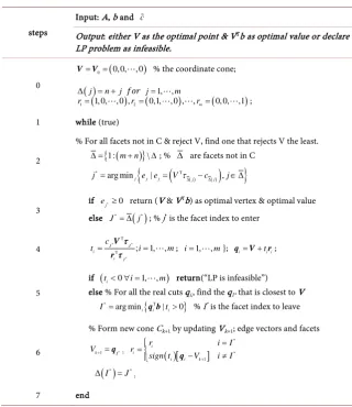
Table 1. Cone-cutting algorithm.
steps
Input: A, b and c
Output: either V as the optimal point & VTb as optimal value or declare the
LP problem as infeasible.
0
( )
0 0, 0, , 0 = =
V V % the coordinate cone;
( )j n j
∆ = + 𝑓𝑓𝑓𝑓𝑓𝑓 j=1,,m
( ) ( ) ( )
1 1, 0, , 0 ,2 0,1, , 0 , ,m 0, 0, ,1
r= r = r = ;
1 while (true)
2
% For all facets not in C & reject V, find one that rejects V the least. ∆ =
{
1:(m+n)}
\∆; % ∆ are facets not in C
{
(
( ) ( ))
}
* T
arg minj j| j j j ,
j = e e = V τ∆ −c∆ j∈ ∆
3 if ej*≥0 return (V & V
Tb) as optimal vertex & optimal value
else *
( )
*J = ∆ j ; % j* is the facet index to enter
4 * * *
T T
; 1, ,
i J J i
J c
t = V i= m
r
τ
τ ; i=1,,m}; qi= +V ti ir;
5
if (ti< ∀ =0 i 1,,m) return(“LP is infeasible”)
else % For all the real cuts qi,, find the qI* that is closest to V
*
{
T}
arg mini i | i 0
I = q b t > % I* is the facet index to leave
6
% Form new cone Ck+1 by updating Vk+1; edge vectors and facets
Vk+1=qI*; ( )
[
]
* * 1
i i
i i k
r i I
r
sign t V+ i I
=
= − ≠
q Δ
( )
* *I =J ;
7 end
vertex of a new cone. This new cone retains all the facets of the original cone ex-cept that the cutting facet replaces the facet corresponding to the edge I*. Yet the
edge I* is retained but the rest of the edges must be recomputed as shown in step
6. Amazingly, P.Z. Wang shows that when b>0, this algorithm produces ex-actly the same result as the original simplex algorithm proposed by Dantz [2]. Hence, the cone-cutting theory offers a geometric interpretation of the simplex method. More significantly, it inspires the authors to explore new approach to tackle the LP problem.
3. Sliding Gradient Algorithm
Expanding on the cone-cutting theory, the Gravity Sliding Algorithm [1] was developed to find the optimal solution of the LP problem from a point within the feasible region 𝒟𝒟. Since then, several refinements have been made and they are presented in the following sections.
DOI: 10.4236/ajor.2018.82009 118 American Journal of Operations Research
(
T ;1)
j≥cj ≤ ≤ +j n m
y τ , and the optimal feasible point is at one of its vertices.
Let
{
T}
| ; 1, ,
i i j cj j n m
Ω = V V τ ≥ = + be the set of feasible vertices. The dual LP problem (3) can then be stated as: min
{
T |}
i
i ∈Ω
V b V . As
V b
iT is thein-ner-product of vertex Vi and b, the optimal vertex *
V is the vertex that yields the lowest inner-product value. Thus we can set the principle descending direc-tion g0 to be the opposite of the b vector (i.e. g0= −b) and this is referred to
as the gravity vector. The descending path then descends along this principle di-rection inside 𝒟𝒟 until it reaches the lowest point in 𝒟𝒟 viewed along the direction of b. This point is then the optimal vertex *
V .
3.2. Circumventing Blocking Facets
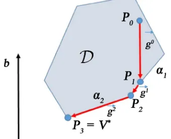
The basic principle of the new algorithm can be illustrated in Figure 2. Notice that in 2-dim, a facet is a line. In this figure, these facets (lines) form a closed polyhedron which is the dual feasible region 𝒟𝒟. Here the initial point P0 is inside
𝒟𝒟. From P0, it attempts to descend along the g0= −b direction. It can go as far
as P1 which is the point of intersection between the ray R=P0+tg0 and the
facet α1. In essence, α1 is blocking this ray and hence it is called the blocking facet
relative to this ray. In order not to penetrate 𝒟𝒟, the descending direction needs to change from g0 to g1 at P1, and slides along g1 until it hits the other blocking
facet α2 at P2. Then it needs to change course again and slides along the direction
g2 until it hits P3. In this figure, P3 is the lowest point in this dual feasible region
𝒟𝒟 and hence it is the optimal point *
V .
It can be observed from Figure 2 that g1 is the projection of g0 onto α1 and g2
is the projection of g0 onto α2. Thus from P1, the descending path slides along α1
to reach P2 and then slides along α2 to reach P3. Hence we call this algorithm
Sliding Gradient Algorithm. The basic idea is to compute the new descending direction to circumvent the blocking facets, and advance to find the next one until it reaches the bottom vertex viewed along the direction of b.
Let σt denotes the set of blocking facets at the t
thiteration. From an initial
point P0 and a gradient descend vector g0, the algorithm iteratively performs the
following steps:
[image:7.595.289.459.568.706.2]1) compute a gradient direction gt based on σt. In this example, the initial set
DOI: 10.4236/ajor.2018.82009 119 American Journal of Operations Research of blocking facets σ0 is empty and g0= −b.
2) move Pt to Pt+1 along gt where Pt+1 is a point at the first blocking
facet.
3) Incorporate the newly encountered blocking facet to σt to form σt+1.
4) go back to step 1.
The algorithm stops when it cannot find any direction to descend in step (1). This is discussed in details in Section 3.6 where a formal stopping criterion is given.
3.3. Minimum Requirements for the Gradient Direction
g
tFor the first step, the gradient descend vector gt needs to satisfy the following
requirements.
Proposition 1. gt must satisfy
( )
T
0 0
t ≥
g g so that the dual objective func-tion T
y b
will be non-increasing when y move from Pt to Pt+1 along thedi-rection of gt.
Proof. Since
( )
T0 0
t ≥
g g , gt aligns to the principle direction of g0. As 1
t+ = +t t t
P P g , Pt+1 moves along the principle direction of g0 when t>0.
Since T T
( )
T T( )
T1 0
t+ = t +t t = t −t t
P b P b g b P b g g ,
P b
tT+1≤
P b
tT when( )
T
0 0
t ≥
g g .
END
This means that if
( )
T0 0
t ≥
g g , then Pt+1 is “lower than” Pt when viewed
along the b direction.
Proposition 2. If P0∈, gt must satisfy
( )
( ) T0
t j t
σ
τ
g ≥ for all j∈σt toensure that Pt+1 remains dual feasible (i.e. Pt+1∈).
Proof. If for some j,
( )
( )T
0
t j t
σ
τ
g < , this means that gt is in the opposite direction of the normal vector of facetα
σt( )j so a ray Q=Pt+tgt willeven-tually penetrate this facet for certain positive value of t. This means that Q will be rejected by
α
σt( )j and hence Q is no longer a dual feasible point. END3.4. Maximum Descend in Each Iteration
To ensure that Pt+1∈, we need to make sure that it won’t advance too far. The
following proposition stipulates the requirement.
Proposition 3. Assuming that 𝒟𝒟 is non-empty and P0∈. If gt satisfies
Propositions 1 and 2; and not all T
0
t j =
g
τ
for j=1,,m+n, then Pt+1∈provided that the next point Pt+1 is determined according to (6) below:
* 1
t+ = +t tj t
P P g
(6)
where
T *
T
arg minj j| j j t j; j 0; 1, ,
t j
c
j = t t = t > j= m+n
−
P
g
τ
τ .
Proof. The equation for a line passing through P along the direction g is t
+
P g. If this line is not parallel to the plane (i.e.
g
Tτ
≠
0
), it will intersect afacet
α τ
:
( )
,
c
at a point Q according to the following equation:(
T)
Twhere
t t c
= + = −
Q P g P τ g τ.
DOI: 10.4236/ajor.2018.82009 120 American Journal of Operations Research We call t the displacement from P to Q. So
T
T
j t j
j
t j
c t = −P
g
τ
τ
is the displace-ment from Pt to αj. The condition tj > 0 ensures that Pt+1 moves along thedirection gt but not the opposite direction. *
j
is the smallest of all the dis-placements thusα
j* is the first blocking facet that is closest to Pt.To show that Pt+1∈, we need to show T
1 0
t+ j− ≥cj
P
τ
for j=1,,m+n. Note that(
*)
(
)
*T
T T T
1
t+ j −cj = t +tj t j−cj = t j−cj +tj t j
P τ P g τ P τ g τ .
Since Pt∈,
(
)
T 0
t j −cj ≥
P τ for j=1,,m+n, so we need to show that
* T
0
t j
j
t gτ ≥ for j=1,,m+n.
The displacements tj can be split into two groups. For those displacements
where tj <0,
T
T 0
j t j
j t j c t = − < P g
τ
τ
so gtTτj =(
cj−PtTτj)
tj = −(
cj−PtTτj)
k1 , where k1= −tj is a positive constant. Since tj*>0.(
) (
)
*
*
T T T
2 1
0
j
t j j t j t j j
j
t
t c k c
k
= − − = − ≥
g
τ
Pτ
Pτ
since Pt∈ & k2>0.For those displacements where tj ≥0, we have that tj* is the minimum of
all tj in this group. Let k3 be the ratio between tj* and tj . Obviously,
* 3 1 j j t k t = ≤
(
)
(
)
(
)
(
) (
)
* T T TT T T T
3 3 T
T T
3 0
t j j j t j
j t j
t j j j t j t j j t j
t j
t j j t j j
c t
c
c k t c k
c k c
− + = − + = − + = − − − ≥ − P g P
P g P g
g
P P
τ τ
τ
τ τ τ τ
τ
τ τ
So Pt+1∈. END
If T
0
t j =
g
τ
, gt is parallel to αj. Unless all facets are parallel to gt,Propo-sition 3 can still find the next descend point Pt+1. If all facets are parallel to gt,
this means that facets are linearly dependent with each other. The LP problem is not well formulated.
3.5. Gradient Projection
We now show that the projection of g0 onto the set of blocking facets σt
sa-tisfies the requirements of Proposition 1 and 2. Before we do so, we discuss the projection operations in subspace first.
3.5.1. Projection in Subspaces
Projection is a basic concept defined in vector space. Since we are only interested in the gradient descend direction of gt but not the actual location of the
pro-jection, we can ignore the constant c in the hyperplane
{
T}
| =cDOI: 10.4236/ajor.2018.82009 121 American Journal of Operations Research words, we focus on the subspace
V
( )
τ
spanned by τ and its null space( )
N
τ
rather than the affine space spanned by the hyperplanes.Let Y be the vector space in m,
V
( ) {
τ =
y y
|
=
t t
τ
;
∈
}
and itscorres-ponding null space is N
( )
τ ={
x x y| T =0 forx∈Yand y∈V( )
τ}
. Extending to k hyperplanes, we have(
1, 2, ,)
{
| ;}
k
k j j j j
V
τ τ
τ
= y y=∑
tτ
t ∈R and the nullspace is
(
)
{
T(
)
}
1, 2, , k | 0 for and 1, 2, , k
N τ τ τ = x x y= x∈Y y∈V τ τ τ . It can be
shown that
N
(
τ τ
1, ,
2
,
τ
k)
=
N
( )
τ
1
N
( )
τ
2
N
( )
τ
k . SinceV
(
τ τ
1, ,
2
,
τ
k)
and
N
(
τ τ
1,
2,
,
τ
k)
are the orthogonal decomposition of the whole space Y, avector g in m can be decomposed into two components: the projection of g
onto
V
(
τ τ
1, ,
2
,
τ
k)
and the projection of g ontoN
(
τ τ
1, ,
2
,
τ
k)
. We use thenotation g↓[τ τ1,2, ,τk] and g↓α1αk to denote them and they are called direct
projection and null projection respectively.
The following definition and theorem were first presented in [1] and is re-peated here for completeness.
Let the set of all subspaces of m
Y= be 𝒩𝒩, and let 𝒪𝒪 stand for 0-dim sub-space, we now give an axiomatic definition of projection.
Definition 3. The projection defined on a vector space Y is a mapping
#:Y Y
∗ ↓ × →
where ∗ is a vector in Y, # is a subspace X in 𝒩𝒩satisfying that (N.1) (Reflectivity).
For any g∈Y,g↓ =Y g; (N.2) (Orthogonal additivity).
For any g∈Y and subspaces X Z, ∈ , if X and Z are orthogonal to each other, then g↓ + ↓ = ↓X g Z g X Z+ , where X +Z is the direct sum of X and Z.
(N.3) (Transitivity).
For any g∈Y and subspaces X Z, ∈,
(
g↓X)
↓XZ= g↓XZ, (N.4) (Attribution).For any g∈Y and subspace X∈ , g↓ ∈X X , and especially,
(N.5) For any g∈Y and subspace X∈ ,
g g
T↓ ≥
X0
.A convention approach to find g↓α1αk is to compute it directly from the
null space
N
(
τ τ
1,
2,
,
τ
k)
. We now show another approach that is moresuita-ble to our overall algorithm.
Theorem 1. For any g∈Y, we have
1
T
k
k
i i
α α
↓ = −
∑
g g g o
(8) where
{
o
1,
,
o
k}
are an orthonormal basis of subspaceV
(
τ τ
1, ,
2
,
τ
k)
.Proof. Since α1αk and
[
τ τ
1, ,
2
,
τ
k]
are the orthonormaldecompo-sition of Y, according to (N.2) and (N.1) we have [τ1, ,τk] α1 αk
= ↓ + ↓
g g g .
DOI: 10.4236/ajor.2018.82009 122 American Journal of Operations Research
[1 ]
T T
1
, ,k k
τ τ
↓ = + +
g g o g o .
Hence (8) is true. END
The following theorem shows that the projection of g0 onto the set of all
blocking facets σt always satisfies Propositions 1 and 2. First, let us simplify the
notation and use σ to represent σt in the following section and g0↓σ to stand for g0↓ασ( )1ασ( )k where
k
=
σ
is the number of elements in σ.Theorem 2.
( )
( )(
)
T
0 0
j σ
σ
τ
g ↓ = and T(
0)
0 ↓ ≥σ 0
g g for all j=1,,k. Proof. Since g0↓σ lies on the intersection of
(
ασ( )1 ασ( )k)
, it lies on each facetα
σ( )j for j=1,,k. Thus g0↓σ is perpendicular to the normalvector of
α
σ( )j (i.e.( )
( )(
)
T0 0
j σ
σ
τ
g ↓ = ). So it satisfies Proposition 2.According to (N.5), T
(
)
0 0↓ ≥σ 0g g . So it satisfies proposition 1 too. END As such, g0↓σ, the projection of g0 onto all the blocking facets, can be
adopted as the next gradient descend vector gt. Hence, g0↓σ, the projection of g0 onto all the blocking facets, can be adopted as the next gradient descend
vector gt.
3.5.2. Selecting the Sliding Gradient
In this section, we explore other projection vectors which also satisfy Proposi-tions 1 and 2. Let the jth complement blocking set c
j
σ
be the blocking set σ ex-cluding the jth element; i.e.1 1 1
c
j j j k
σ
=α
α
− α
+ α
. We examine the projection 0 cj
σ ↓
g for j=1,,k. Obviously, T
( )
0 0 c 0
j
σ ↓ ≥
g g according to
(N.5) as 0 c j
σ ↓
g is a projection of g0. So if
( )
( )( )
T
0 c 0
j
j
σ σ
τ g ↓ ≥ for all j∈σ, it satisfies Proposition 2 and hence is a candidate for consideration. For all the candidates, including g0↓σ, which satisfy this proposition, we can compute the inner product of each candidate with the initial gradient descend vector g0, (i.e.
( )
T
0 0 c
j
σ ↓
g g ) and select the maximum. This inner product is a measure of how close or similar a candidate is to g0 so taking the maximum means getting the
steepest descend gradient. Notice that if a particular 0 c j
σ ↓
g is selected as the next gradient descending vector, the corresponding αj is no longer a blocking facet in computing 0 c
j
σ ↓
g . Thus αj needs to be removed from σt to form
the set of effective blocking facets * t
σ
. The set of blocking facets for the next ite-ration σt+1 is* t
σ
plus the newly encountered blocking facet. In summary, the next gradient descend vector gt is:(
)
( )
[ ]( )
[ ]( )
[ ](
T T T T)
0 0 0 1 0 2 0
max , , , ,
t= ↓σ k
g g g g g g g g g
(9) where [ ] 0 c;
j
j = ↓σ j∈σ
g g with
( )
( )( )
T
0 c 0
j
j
σ σ
τ g ↓ ≥ and
k
=
σ
.The effective blocking set * t
σ
is{ }
1 0*
1 0
if
\ if c
j
t t
t
t j t
σ σ σ σ σ α + + = ↓ = = ↓ g g
g g .
DOI: 10.4236/ajor.2018.82009 123 American Journal of Operations Research At first, this seems to increase the computation load substantially. However, we now show that once g0↓σ is computed, 0 c
j
σ ↓
g can be obtained efficiently.
3.5.3. Computing the Gradient Projection Vectors
This session discusses a method of computing g↓σ and c j
σ ↓
g for any vector g. According to (8), 1
T
k
k i i
σ α α
↓ = ↓ = −
∑
g g g g o . The orthonormal basis
{
o o
1,
2,
,
o
k}
can be obtained from the Gram Schmidt procedure as follows:1
=
1;
1=
1 1o
τ
o
o
o
(11)
T
2= −2 2 1; 2= 2 2
o
τ τ
o o o o(12) Let us introduce the notation a↓b to denote the projection of vector a onto
vector b. We have TT
↓ =
a b
a b b
b b , then o2=τ2−τ2↓o1 as
( )
T 1 1 =1
o o . Like-wise,
1
1
;
j
j j j i j j j
i
−
=
= −
∑
↓ =o
τ
τ
o o o o .(13) Thus from (8),
T 1 k k i i i i σ = ↓ = −
∑
= −∑
↓g g g o g g o.
(14) After evaluating g↓σ, we can find c
j
σ ↓
g backward from j=k to 1. Firstly,
1 1 c k k i k i σ σ − = ↓ = −
∑
↓ = ↓ + ↓g g g o g g o .
(15) Likewise, it can be shown that
( ) 1
1 1
for 2 to
c j
j k
j
i i
i i j
j k
σ
−
= = +
↓ = −
∑
↓ −∑
↓ =g g g o g o .
(16) The first summation is projections of g onto existing orthonormal basis oi.
Each term in this summation has already been computed before and hence is readily available. However, the second summation is projections on new basis
( )j i
o . Each of these basis must be re-computed as the facet αj is skipped in
σ
cj.Let
; 0
k k k
T = + ↓g g o S = (17)
( ) 1 1 ; k j
j j j j i
i j
T T+ S
= +
= + ↓g o =
∑
g↓o .(18) Then we can obtain c
j
σ ↓
g recursively from j=k k, −1,,1 by:
c
j j j
T S
σ ↓ = −
g .
(19) To compute ( )j
i
o , some of the intermediate results in obtaining the ortho-normal basis can also be reused.
Let µj,1=0 for all j=2,,k and
µ
j i,=
µ
j i, 1−+ ↓
τ
jo
i for i=1,,j−1,then we have
, 1; for 2, ,
j= j−µj j− j= j j j= k
o τ o o o .
DOI: 10.4236/ajor.2018.82009 124 American Journal of Operations Research The intermediate terms µj i, can be reused in computing
( )j m
o as follows:
( ) ( ) ( ) ( )
( ) 1
, 1 1
; for 1, ,
j m
j j j m
m m m j m i m j
i j m
m k
µ − −
= +
= − −
∑
↓ = o = + o o o
o
τ τ .
(21)
By using these intermediate results, the computation load can be reduced sub-stantially.
3.6. Termination Criterion
When a new blocking facet is encountered, it will be added to the existing set of blocking facets. Hence both σt and
*
t
σ will typically grow in each iteration unless one of the 0 c
j
σ
↓
g is selected as gt. In this case,
α
σ( )j is deleted from tσ according to (10). The following theorem, which was first presented in [1]
shows that when *
t m
σ = , the algorithm can stop.
Theorem 3 (Stopping criterion) Assuming that the dual feasible region 𝒟𝒟 is non-empty, let Pt∈ and is descending along the initial direction g0= −b;
let *
t
σ be the number of effective blocking facets in * t
σ
at the tth iteration. If*
t m
σ = and the rank
( )
*t
r σ =m, then Pt is a lowest point in the dual
feasi-ble region 𝒟𝒟. Proof. If *
t m
σ = and the rank
( )
*t
r σ =m, then the m facets in
σ
*t form acone C with vertex V =Pt. Since the rank is m, its corresponding null space
contains only the zero vector. So g0↓ =σ g0↓ασ( )1ασ( )k =0.
As mentioned about the facet/edge duality in Section 2, for j=1,,m, edge-line
R
i+ is the intersection of all C-facets except
i
α . That means c
i i
R
+=
σ
. Since an edge-line is a 1-dimensional line, the projection of a vector0
g onto
R
i+ equals to
i
±r and hence c i i
t ↓ =σ t ↓ = ±R+ i
g g r. Since c
i
t ↓σ
g are projections of g0, according to (N.5),
(
)
T
0 c 0
i
t ↓σ ≥
g g .
Since *
t m
σ = , it means that c i
t↓σ
g does not satisfy Proposition 2 for all
1, ,
i= m. Otherwise, one of the c i
t ↓σ
g would have been selected as the next gradient descend vector and, according to (10), it would be deleted from *
t
σ
and hence *t
σ would be less than m. This means that at least one of j∈σ has a value T
(
)
0
c i
j gt↓σ <
τ
. However, for all k≠i, ci
t ↓σ
g is in the null space of 𝛼𝛼𝑘𝑘 so T
(
c)
0i
k gt↓σ =
τ
. This leaves T(
)
0
c i
i gt↓σ <
τ
. If ci
t↓ =σ i
g r , then
(
)
T T
0
c i
i gt↓σ = iri<
τ
τ
. This contradicts to the fact that T0
i
r
i≥
τ
in (1).There-fore, c
j
t ↓ = −σ i
g r. Since 0T
(
c)
0i
t ↓σ ≥
g g , T
( ) (
)
T0 −i = − 0 i≥0
g r g r . Note that
(
)
T0 i
−g r means that edge ri is in opposite direction of g0. As this is true for
all edges, there is no path for gt to descend further from this vertex. It is
ob-vious that the vertex V is the lowest point of C when viewed in the b direction. Since Pt is dual feasible, and V is a vertex of 𝒟𝒟. Cone C coincides with the
dual feasible region 𝒟𝒟 in a neighborhood N of V, it is obvious that Pt is the
DOI: 10.4236/ajor.2018.82009 125 American Journal of Operations Research In essence, when the optimal vertex *
V is reached, all the edges of the cone will be in opposite direction of the gradient vector g0= −b. There is no path to
descend further so the algorithm terminates.
4. The Pseudo Code of the Sliding Gradient Algorithm
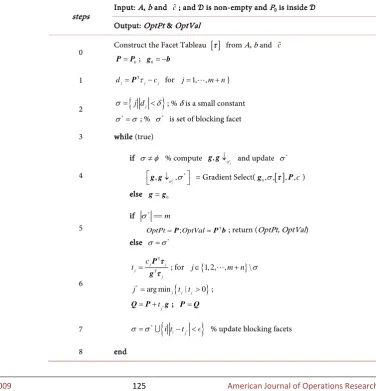
The entire algorithm is summarized as follows in Table 2.
Step 0 is the initialization step that sets up the tableau and the starting point P. Step 2 is to find a set of initial blocking facets σ in preparation of step 4. In the inner loop, Step 4 calls the Gradient Select routine. It computes g0↓σ and
0 c
j
σ ↓
g in view of σ using Equations (11) to (21) and select the best gradient vector g according to (9). This routine not only returns g but also the effective blocking facets σ* and
0 c
j
σ ↓
g for subsequent use. Theorem 3 states that when the size of σ* reaches m, the optimal point is reached. So when it does,
step 5 returns the optimal point and the optimal value to the calling routine. Step 6 is to find the closest blocking facet according to (6). Because P lies on every fa-cets of σ, tj=0 for j∈σ. Hence, we only need to compute those tj where
[image:14.595.158.535.360.752.2]j∉σ. The newly found blocking facet is then included in σ in step 7 and the
Table 2. The sliding gradient algorithm.
steps Input: A, b and c; and 𝒟𝒟 is non-empty and P0 is inside 𝒟𝒟 Output: OptPt & OptVal
0 Construct the Facet Tableau
[ ]
τ from A, b and c0 =
P P ; g0= −b
1 T
j j j
d =Pτ −c for j=1,,m+n}
2 σ=
{
j dj <δ}
; % δ is a small constant*
σ =σ ; % σ* is set of blocking facet
3 while (true)
4
if σ φ≠ % compute , c j σ
↓
g g and update σ*
*
, , c
j
σ σ
↓
g g = Gradient Select(g0, ,σ
[ ]
τ , ,Pc)else g=g0
5
if *
m
σ ==
T
;
OptPt=POptVal=P b; return (OptPt, OptVal)
else σ σ= *
6
T T
j j j
j c
t = P
g
τ
τ ; for j∈{1, 2,,m+n}\σ
{
}
*
arg minj j| j 0
j = t t > ;
* j t
= +
Q P g; P=Q
7
{
*}
*
i j i t t
σ σ= − < % update blocking facets
DOI: 10.4236/ajor.2018.82009 126 American Journal of Operations Research inner loop is repeated until the optimal vertex is found.
5. Implementation and Experimental Results
5.1. Experiment on the Klee-Minty Problem
We use the Klee-Minty example presented in [18]1 to walk through the
algo-rithm in this section. An example of the Klee-Minty Polytope example is shown below:
1 2
1 2 1
max 2
m−x
+
2
m−x
+ +
2
x
m−+
x
m. Subject to1
x ≤ 1
5
1
4x + x2 + ≤
2
5
1
8x + 4x2 + x3 ≤
3
5
1
2m
x + 1
2
2m x −
+ 2
3
2m x −
+ xm ≤ 5 m
For the standard simplex method, it needs to visit all 1
2m− vertices to find the optimal solution. Here we show that, with a specific choice of initial point P0,
the Sliding Gradient algorithm can find the optimal solution in two itera-tions—no matter what the dimension m is.
To apply the Sliding Gradient algorithm, we first construct the tableau. For an example with m=5, the simplex tableau is:
1 5
4 1 25
8 4 1 125
16 8 4 625
32 16 8 4 1 3125
16 8 4 2 1
The b vector is
[
]
T5, 25,125, 625, 3125 =
b . After adding the slack variables,
the facet tableau becomes:
α1 α2 α3 α4 α5 α6 α7 α8 α9 α10
1 0 0 0 0 1 0 0 0 0
4 1 0 0 0 0 1 0 0 0
8 4 1 0 0 0 0 1 0 0
16 8 4 1 0 0 0 0 1 0
32 16 8 4 1 0 0 0 0 1
16 8 4 2 1 0 0 0 0 0
1Other derivations of the Klee-Minty formulas have also been tested and the same results are
DOI: 10.4236/ajor.2018.82009 127 American Journal of Operations Research Firstly, notice that α5 and α10 have the same normal vector (i.e. τ5=τ10)
so we can ignore α10 for further consideration. This is true for all value of m.
If we choose P0 =Mb, where M is a positive number (e.g. M =100), It can
be shown that P0 is inside the dual feasible region. The initial gradient descend
vector is: g0= −b.
With P0 and g0 as initial conditions, the algorithm proceeds to find the
first blocking facet using (6). The displacements tj for each facet can be found by:
T T
0
T T T T T
0
j j j j j j
j
j j j j j
c c M c c
t = = − = +M=M−
− − −
−P b
g b b b b
τ
τ
τ
τ
τ
τ
τ
.With P0 and g0 as initial conditions, the algorithm proceeds to find the
first blocking facet using (6). The displacements tj for each facet can be found by:
T T
0
T T T T T
0
j j j j j j
j
j j j j j
c c M c c
t = = − = +M =M−
− − −
−P b
g b b b b
τ
τ
τ
τ
τ
τ
τ
.(22)
We now show that the minimum of all displacements is tm.
First of all, at = m,
[
]
T 0, , 0,1m =
τ , cm=1 and
5
m m
b
=
, sot
m=
M
−
5
−m.For m< ≤j 2m−1, cj=0, so tj =M >tm.
For 1≤ <j m, cj 2m j −
= , and the elements of τj are:
1 0 if 1 if 2 if ij i j i j i j
j i m τ
− +
<
= = < ≤
.
The 2nd term of Equation (22) can be re-written as:
T T T 1 1 2 j j j j m j j c c − = = b b b τ τ τ
The inner product of the denominator is:
1
1 1
T
1 1 1
2
2
2 2 2 2 2
m j
m m m
j ij ij ij
i i m i m
m j m j m j m j m j
i i i
b b b b b
− + − − − − − − − = = = = = + = +
∑
∑
∑
b
τ
τ
τ
τ
Since all the elements in the b vector and the τ are positive, the summation is a positive number. Thus
1 T 1 2 2 2 m j ij
i m m
m j m j
i
b
τ
b b−
− −
=
= + >
∑
b
τ
Since the value of the denominator is bigger than
b
m=
5
m, we haveDOI: 10.4236/ajor.2018.82009 128 American Journal of Operations Research T T 1 5 2 j m j m j j m j c
t M M M − t
−
= − = − > − = b b τ τ .
Hence tm is the smallest displacement. For the case of m=5, their values
are shown in the first row (first iteration) of the following Table 3. Thus αm is the closest blocking facet. Hence,
{ }
*
1 1 m
σ
=σ
=α
. For the next iteration,(
)
( )
1 0 0 5 5 5
m m m
m
t M M − M M − −
= + = + − − = − + =
P P g b b b b b b.
The gradient vector g1 is g0 projects onto αm. Because
[
]
T 0, ,1
m=
τ is
already an orthonormal vector, we have according to (8)
(
T)
T 2 1 T1 0 0 0 0, , 5 5, 5 , , 5 , 0
m m
m m
−
= − = − − = − − −
g g gτ τ g .
In other words, g1 is the same as −b except that the last element is zeroed
out. Using P1 and g1, the algorithm proceeds to the next iteration and
eva-luates the displacements tj again. For j= +m 1 to 2m−1, since cj=0 and
j
τ is a unit vector with only one non-zero entry at the jth element, T 1 T T T 1 1 5
5 5 for 1 2 1
m
j j m j m
j
j
j j
b
t m j m
b − − − = − = − = − = + ≤ ≤ − − b g g
P
τ
τ
τ
τ
.Thus the displacements tm to t2m−1 have the same value of 5 m
− . For 1≤ <j m, we have:
T 1
T T T
1 1 1
T T
5 5
5
m m
j j j j m j j
j
j j j
c c c
t
−
−
− − −
= P = b = b
g g g
τ
τ
τ
τ
τ
τ
.As mentioned before, g1 is the same as −b except that the last element is
zero, we can express T j
b
τ
in terms of g1Tτ
j as follows: T1 T
j= − j+bm mj
τ
b
τ
gτ
.The numerator then becomes:
T 1 T
5mcj−b
τ
j =5mcj+gτ
j−bm mjτ
.Since cj 2m j −
= , cj 2m j −
= and 1
2m j
mj
τ
= − +, substituting these values to the above equation, the numerator becomes
T 1 T T
1 1
5mcj j 5 2m m j 5 2m m j j j 5 2m m j
− − + −
−b
τ
= − +gτ
=gτ
− .Thus
T T
1 1
T
5 5 2
5 5 1
m m m j
j j m m j j j c t − − − − = = − b g g τ
[image:17.595.280.470.75.114.2] [image:17.595.167.541.120.757.2]τ τ .
Table 3. Displacement values ti in each iterations for m=5.
t1 t2 t3 t4 t5 t6 t7 t8 t9
DOI: 10.4236/ajor.2018.82009 129 American Journal of Operations Research Notice that all elements in g1 are negative but all of τj are positive. So the inner product T
1 j
g
τ
is a negative number. As a result, the last term inside the bracket is a positive number which makes the whole value inside the bracket bigger than one and hence tj 5m−
> for 1≤ < −j m 1. Moreover, tm is zero as
1
g lies on αm. The actual displacement values for the case of m=5 are
shown in the second row of Table 3.
Since tm to t2m−1 have the same lowest displacement value, all of them are
blocking facets so *
{ } {
} {
}
2 2 m m1, , 2m1 m, m1, , 2m1
σ
=σ
=α
α
+ α
− =α α
+ α
− . Also,[
]
T T
2 1
2 1 1 1 5 5 5, 5 , , 5 , 0 0, 0, , 0,1
m m m
m
t + − − −
= + = + − − − =
P P g b .
Now *
t m
σ = , so P2 has reached a vertex of a cone. According to Theorem
3, the algorithm stops. The optimal value is T
2
5
m
=
P b
, which is the last elementof the b vector.
Thus with a specific choice of the initial point P0=Mb, the Sliding Gradient
algorithm can solve the Klee-Minsty LP problem in two iterations, and it is in-dependent of m.
5.2. Issues in Algorithm Implementation
The Sliding Gradient Algorithm has been implemented in MATLAB and tested on the Klee-Minty problems and also self-generated LP problems with random coefficients. As a real number can only be represented in finite precision in digi-tal computer, care must be taken to deal with the round-off issue. For example, when a point P lies on a plane
y
Tτ
=
c
, the value Td=P τ−c should be ex-actly zero. But in actual implementation, it may be a very small positive or nega-tive number. Hence in step 2 of the aforementioned algorithm, we need to set a threshold δ so that if
d
<
δ
, we regard that point P is laid on the plane. Like-wise for the Klee-Minty problem, this algorithm relies on the fact that in the second iteration, the displacement values ti for i= +m 1 to 2m−1 shouldbe the same and they should all be smaller than the values of tj for j=1 to 1
m− . Due to round-off errors, we need to set a tolerant level to treat the first
group to be equal and yet if this tolerant level is set too high, then it cannot ex-clude members of the second group. The issue is more acute as m increases. It will require higher and higher precision in setting the tolerant level to distin-guish these two groups.