Automated analysis and simulation of control systems using dataflow

(1)

Automated analysis and simulation of control systems

using dataflow

S. (Silke) Hofstra

MSc

Report

Committee:

Dr.ir. J.F. Broenink

Dr.ir. J.B.C. Engelen

Ir. J. Scholten

December 2018

050RAM2018

Robotics and Mechatronics

EE-Math-CS

University of Twente

(2)

i

Summary

While modern embedded systems development offers many opportun-ities, the design of real-time control systems also poses many chal-lenges. An example of such a challenge is the development process: embedded software engineers and control engineers need to work to-gether to realize a control system, which can be complex from both a control engineering and software engineering standpoint.

To ease this development process, methods like model-driven devel-opment are used. Fitting within this process, this research proposes concrete workflow steps that allow a decoupling between the tasks of the control engineer and the software engineer. The workflow allows autonomy in the development process for the control engineer, who can create a platform-independent model, a platform-specific model and a realization using the tools available.

The goal of this research is to provide a method for converting a platform-independent model into a platform-speciﬁc model automatically, and using this platform-speciﬁc model to reach conclusions about the fu-ture realization.

A look is taken into the existing software solutions and what value they provide in the proposed workflow. Three existing modelling techniques are compared for suitability in the representation of platform-specific models: block diagrams, communicating sequential processes and synchronous dataflow

The proposed solution for the creation of platform-specific models is to convert a block diagram together with a platform and parameters into a synchronous dataflow (SDF) diagram. This SDF model can then be analysed using existing SDF methods for verification of the model. Simulation of this model is used for validation of the model.

This process is implemented in a proof-of-concept tool that can per-form the conversion, analysis and simulation of conﬁgured models. The proof-of-concept tool is used in several example systems to show the functionality, and limitations, of the conversion process. This tool uses a special representation for the plant in order to simulate a full system.

The tool is veriﬁed by analysis against models with known properties. The limitations of the conversion process are shown in the analysis of an ADC element, which has more complex behaviour. It is shown that the tool is able to perform analysis and simulation of the behaviour of a simple PID system. It is also able to perform analysis, but not simulation, on a more complex control system.

(3)

Automated analysis and simulation of control systems using dataﬂow ii

In the future, research needs to be done into improvement of the simu-lation through co-simusimu-lation, improvements of analysis using external libraries, better representation of effects of the platform, and improved representation of components like ADCs and webcams.

(4)

iii

Introduction

Modern embedded systems offer a great deal of opportunities for con-trol engineers: cheap microconcon-trollers (MCUs) and field programmable gate arrays (FPGAs) allow the design of modular hard real-time con-trol systems with more sensor inputs and more actuation signals than ever before. This means that improved workflows and toolchains for getting controller designs onto those embedded systems are more im-portant than ever. The design of such embedded control systems, however, currently requires deep knowledge of both control engineer-ing and embedded systems engineerengineer-ing. Control engineers often design control systems using domain-specific models, which then have to be implemented on the targeted embedded system by (embedded) soft-ware engineers. This requires a process with standardised knowledge, and compatibility, between the worlds of control engineering and soft-ware engineering.

Integration of the design process, where a control engineer is able to use a model and transform this directly to a working implementation, can lead to large improvement in the development time and effort of control systems. There are several toolchains that aim to do just this, such as theTwente Embedded Real-time Robotic Application(TERRA) (Bezemer, ), -sim(Kleijn, Groothuis and H.G, ), andSimulink

(MathWorks, ). Most of these toolchains target only general pur-pose processors or speciﬁc platforms, and not generally available mi-crocontrollers and FPGA platforms. The design of ‘hybrid’ controllers, which run parts on different (communicating) platforms, is not pos-sible.

.

Development of a control system

The end goal of the development process of a control system is to design and realize a control system for a real-world application. This design is constraint by the reality of software and hardware, and how these interact.

. .

Architecture

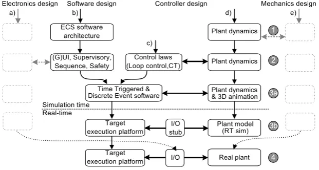
Figure . shows the system architecture of a cyber-physical system— such as a control system. The ﬁgure consists of three parts (Broenink, Ni and Groothuis, ):

(7)

Automated analysis and simulation of control systems using dataﬂow Chapter . Introduction

Figure . :Detailed system architecture of a cyber-physical system (Broenink, Ni and Groothuis, ).

loop control) and non-critical (e.g. user interface) parts of the system. The embedded software runs on a platform, which can be anything from a single-board computer to a microcontroller to an FPGA. Note that, for the purpose of this report, this part in-cludes any programmable part of an FPGA that does not perform input/output (I/O) directly.

• I/O hardwarecontains all interfacing from the digital to physical domain, and vice-versa. This hardware is usually present on the platform on which the software runs.

• Processorplantcontains the physical system, the actuation that controls the physical system, and the sensors that measure the physical system.

Such a system is usually developed by acontrol engineerand an (em-bedded)software engineer: the control engineer creates models of both the controller and plant, and the software engineer creates an im-plementation of the controller on an embedded platform.

. .

Validation and veriﬁcation

Both thevalidationandveriﬁcationof the system are important, these terms are deﬁned as follows (IEEE, ):

• Validationis the assurance that the system meets the needs of the customer and other identiﬁed stakeholders. In concrete terms for a control system, this means that the system can control what is to be controlled (i.e. the plant). An important component of the validation process is simulation using a model of the plant, and testing of the system against the actual plant.

• Verificationis the evaluation of whether or not the system com-plies with the requirements or specification. This is often an in-ternal process. In the context of this report this is interpreted as verification that the realized system matches requirements and functionality of the modelled system.

. .

Workﬂow

The development of a control system is often based on the principles of model-driven development (MDD) (Hailpern and Tarr, 6) or model-driven engineering (MDE) (Schmidt, 6). In this development pro-cess, the control engineer creates a platform-independent model (PIM) of the control system, and a model of the plant, using domain-speciﬁc modelling (DSM). In combination with the chosen platform, and work-ing together with a software engineer, this information is then used to create a platform-speciﬁc model (PSM) as a basis of the implementa-tion of the system.

[image:7.595.62.369.71.167.2]

(8)

Figure . :Concurrent design workﬂow (Broenink, Ni and Groothuis, ).

software for a cyber-physical system, as described in Broenink, Ni and Groothuis ( ). For the development of a control system into an ap-plication, branchesbandcreﬂect the development of the controller. The model of the plant and then the plant itself, in thedbranch, are used forvalidationof the steps: does the control system behave as re-quired and intended? In the way of working shown, the work at the start of development is performed separately by the software engineer and control engineer: the software engineer (branchb) starts by designing an architectural overview and developing several high level tasks, while the control engineer is modelling the plant and applying control theory (step and , indicated on the right). In the third step ( a and b) the controller design is realized for the target platform. The fourth and last step is the actual realization of the design. In this process, knowledge and experience about control engineering is required from the (embed-ded) software engineer, and knowledge about software engineering is required from the control engineer.

. .

Separation of concerns

Figure . :The “Five Cs” of separations of concerns in the design of complex robotics systems (Bruyninckx et al.,

).

The separation of concerns for a project can be described by the “ Cs”, shown in ﬁgure . (Bruyninckx et al., ):

• Computationcontains the implementation of the components of the system.

• Communicationdescribes how data is communicated between components.

• Connection is the speciﬁcation of how components should be connected.

• Coordinationdescribes how the activities of components should work togther.

[image:8.595.60.371.71.237.2]

(9)

This is beneﬁcial to structure the model-driven design of a control sys-tem, and provides a structure for the automation of (parts of) the pro-cess.

.

Proposed workﬂow

As a solution to the issues identified at the start of this chapter, a new workflow is proposed. The goals of this workflow are twofold: (i) give control engineers autonomy to transform models to code, and (ii) allow design of controllers spanning one or multiple platforms.

In order to reach these goals an approach is required that facilitates a structured and incremental approach to controller design, and allows control engineers to design a control system and implement it with minimal knowledge of the underlying platform.

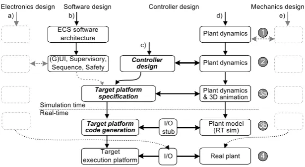
The proposed workﬂow consists of the following stages:

. Controller design:the control engineer designs a platform-independent model of the control system. This design is validated by simula-tion against a model of the plant.

. Target platform specification: the target platform is specified by the control engineer, which—together with the platform-independent model of the previous step—leads to a platform-specific model of the control system that can be verified with analysis and val-idated by simulation against a model of the plant.

. Target platform code generation: the platform-speciﬁc model is used to create a realization of the control system for the target platform. This realization can be deployed to the target platform, and tested against a model of the plant (e.g. via an I/O stub) or the real plant.

Figure . :Proposed workflow shown in the workflow from figure . . The three steps of the proposed workflow are highlighted in bold.

[image:9.595.61.369.456.624.2]

(10)

developerof a toolchain that allows the control engineer to design the entire system by themselves.

.

Research

The focus of this report is on the second step of the proposed work-flow: the analysis and validation of the system when given a platform-independent model and information about the platform. The first step— controller design—is covered by existing solutions (chapter ), and the third step—target platform code generation—is left as future work. This means the following question needs to be answered: how can one automatically create a specific model based on a platform-independent model and platform information, and automatically per-form analysis on, and simulation of, this platper-form-specific model?

To answer this, the following questions need to be, and are, answered in the following chapters:

• What are existing software solutions that provide means to real-ize a platform-independent model on a platform, and in what re-gard are they suitable for analysis and simulation of the designed system? (Chapter )

• What is the most suitable modelling method for a platform-speciﬁc model for analysis and simulation? (Chapter )

• How can a platform-independent model be converted into an (ana-lysable) platform-speciﬁc model? (Chapter )

• How can the constraints of the platform be represented in the platform-speciﬁc model? (Chapter and )

• What information is required to automatically transform a platform-independent model into a platform-speciﬁc model? (Chapter )

• What meaningful feedback can be given to the control engineer based on analysis of the platform-speciﬁc model? (Chapter and )

• How can the real-time behaviour of the platform-speciﬁc model be simulated? (Chapter )

.

Outline

Currently available software solutions that ﬁt into the paradigms dis-cussed in the previous sections are disdis-cussed in chapter .

Modelling methods used for the modelling of real-time and/or control-systems—block diagrams, communicating sequential processes (CSP) and synchonous dataﬂow (SDF)—are compared in chapter .

A way of converting a platform-independent model in the form of a block diagram into a platform-speciﬁc model in the form of SDF is pro-posed in chapter .

A proof-of-concept software tool that automatically performs this con-version and analysis on the resulting model is described in chapter .

The proposed methods and developed tool are evaluated in chapter6

using various examples.

(11)

6

Chapter

State of the art

The following sections describe the tools that are currently used for high-level—usually model-driven—design of (embedded) control sys-tems. This includes both tools that are currently used for model-driven design of control systems, the techniques these tools use, and tools that exist for implementing control systems in software and/or hard-ware. The three tools in this comparison are -sim, Simulink and

TERRA. -sim and TERRA originate at the University of Twente and have been explicitly developed for control engineers (Broenink, ; Bezemer, ). -sim is being developed by Controllab Products. This contrasts with Simulink, the most popular commercial product in this space, which is a part of MATLAB and developed by MathWorks.

.

-SIM

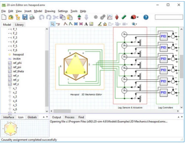
Figure . :Image of the -sim inter-face showing a robot model (Controllab,

8).

-sim is “a modelling and simulation program for mechatronic sys-tems” currently developed and distributed by Controllab (Controllab,

[image:11.595.63.371.447.685.2]

(12)

Automated analysis and simulation of control systems using dataﬂow Chapter . State of the art

control system and its properties. -sim can export models to MAT-LAB, Simulink, and C-code (Kleijn, Groothuis and H.G, ). The latter targets both embedded platforms like Arduino/AVR, and other applic-ations.

-sim C extends this functionality with a rapid-prototyping environ-ment which allows retime interaction with a control system, and al-lows the integration of generated C-code that can be used for interfa-cing with sensors and running the controller (Kleijn, ). The C-code requires an underlying operating system, and the rapid-prototyping plat-form requires a speciﬁc operating system with live communication.

-sim ( C), therefore, has two supported approaches to deploying a model to a hardware platform:

. Export of C-code and using this in a custom project. This still requires all details of the platform to be integrated by the de-veloper, but can be used on any platform that can run C code: this includes soft-cores on FPGAs.

. Using the -sim C rapid prototyping platform to run the model on a suitable platform. This requires almost zero knowledge of embedded systems, but only works on supported platforms like the TS- , or (with more knowledge required) a PC/ com-pliant PC.

. It is not possible to create a design targeting both embedded pro-cessorandFPGA.

.

Simulink

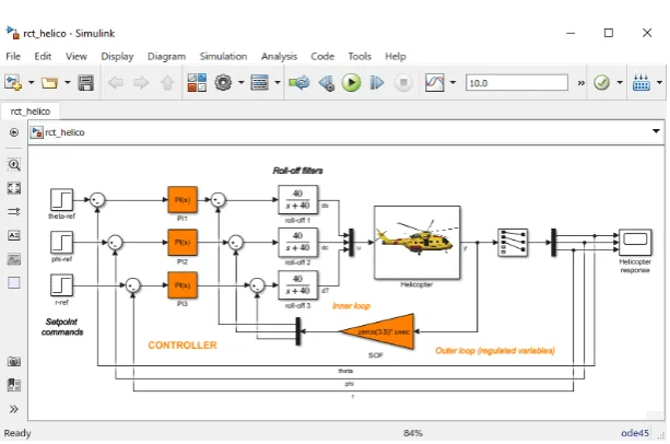
Figure . :Image of the simulink in-terface showing a helicopter controller (Mathworks, 8).

Simulink is an environment for modelling and simulating embedded systems, developed by Mathworks (MathWorks, ). Simulink uses block diagrams to model systems, where blocks can be integrated with custom-build MATLAB code.

Simulink Coder allows the generation and execution of C and C++ code from Simulink models. Supported hardware platforms for running code include many popular microcontrollers likeSTM NucleoandArduino

boards (MathWorks, 8). Simulink HDL Coder allows the generation of code targeting FPGAs (MathWorks, 8).

[image:12.595.63.370.418.621.2]

(13)

Automated analysis and simulation of control systems using dataﬂow Chapter . State of the art 8

. Export of C, C++, VHDL or Verilog code based on the MATLAB/Sim-ulink models to integrate in larger projects or run on unsupported hardware.

. Using Simulink on a supported platform, which can be a GPP, MCU or FPGA.

. It is not possible to create a design targeting both embedded pro-cessorandFPGA.

.

TERRA / LUNA

The Twente Embedded Real-time Robotic Application (TERRA) (Beze-mer, ) is a tool suite for model-driven design of cyber-physical sys-tems. It allows for design usingCommunicating Sequential Processes

(CSP) and architecture models. TERRA aims to achieve aﬁrst-time rightimplementation. The model consists of a network of compon-ents with basic functionality provided by aGeneric Architecture Com-ponent(GAC). TERRA has also been extended with simulation support (Lu, Ran and Broenink, 6).

The LUNA Universal Network Architecture (LUNA) (Bezemer and Wil-terdink, ) is an execution framework that enables the conversion of models to C++ code suitable for several operating systems. LUNA enables the hard real-time design for (CPU-based) hardware platforms, and operating systems. The code generation can be used to imple-ment a controller on any (supported) platform.

. .

CλaSH

CλaSH (clash-lang.org, 8) is a functional hardware description lan-guage built on Haskell. CλaSH enables a relatively high-level approach to hardware design by allowing a functional behavioural description of the signal processing that should be performed. This high-level ap-proach allows rapid development of any kind of signal processing, in-cluding control systems.

CλaSH has been integrated with the TERRA toolchain in order to easily develop a control system for it, but this has some limitations (Kuipers,

):

• Generated code still has to be adapted by the user to make it usable.

• Instrumentation has to be added by hand to make the setup test-able.

• Adding instrumentation uses a relatively large amount of FPGA resources.

• It is not possible to create a design targeting both embedded pro-cessorandFPGA.

Summarised as (Kuipers, ):

(14)

Automated analysis and simulation of control systems using dataﬂow Chapter . State of the art

Solution

Controller design & simulation

Platform-speciﬁc design & simulation

Code generation

-sim Yes No Yes

Simulink Yes No Yes

TERRA No Yes Yes

Table . :Overview of suitability of evaluated software for the creation and simulation of platform-independent controller models, platform-speciﬁc models and the generation of code for the target platform.

.

Comparison

All three software solutions ﬁt within at most two of the steps in the workﬂow described in section . , which can be seen in table . . Both -sim and Simulink can perform modelling and simulation of given controllers and plants, and can create code for a limited number of platforms. TERRA can simulate a CSP equivalent of a controller and allows code generation.

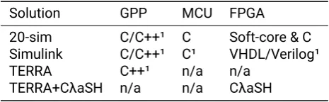
Solution GPP MCU FPGA

-sim C/C++¹ C Soft-core & C Simulink C/C++¹ C¹ VHDL/Verilog¹

TERRA C++¹ n/a n/a

TERRA+CλaSH n/a n/a CλaSH

Table . :Comparison of embedded systems knowledge required when using the examined software solutions for deploying models to platforms.

¹:Zeroembedded systems knowledge is required on a limited number of spe-ciﬁcally supported platforms.

[image:14.595.64.363.72.141.2] [image:14.595.99.332.269.341.2]

(15)

F(s)

X(s) Y(s)

Figure . :Example of ablockin a block diagram with a transfer func-tionF(s)and mathematical relation

Y(s) =X(s)F(s).

x1(t) +

x2(t)

−

y(t)

Figure . :Example of asumming pointin a block diagram, adding two signals with mathematical relation

y(t) =x1(t) +x2(t).

x1(t) x2(t)

x3(t)

Figure . :Example of atake-off point

in a block diagram with mathematical relationx1(t) =x2(t) =x3(t).

Chapter

Modelling techniques

When modelling systems there is a trade-off between analysability and expressiveness: expressive models are hard to analyse, but allow mod-elling everything. Strict techniques are easy to analyse but can express less (Stuijk, Geilen, Theelen et al., ). For the modelling of control systems, three techniques are compared: block diagrams, communic-ating sequential processes and synchronous dataﬂow. All three are used in the development of control systems or the analysis of concur-rent and/or real-time systems.

.

Block diagrams

Block diagrams are the most common way of modelling control sys-tems. Block diagrams can represent the continuous-time and state space behaviour and operations of control systems in discrete ele-ments, where the input-output relationships are indicated (Franklin, Pow-ell and Emami-Naeini, 6, p. ).

The elements of block diagrams are composed of several elements:

• blocks(ﬁgure . ), which represent a transfer function operating on a signal.

• arrows, which indicate the signals and their direction.

• summing points(ﬁgure . ), represented by an open circle, which add or subtract signals. The circle is sometimes ﬁlled by a Σ or cross. Next to the incoming signals, addition or subtraction is indicated. This may also be used formultipliers(i.e.modulators

andmixers), denoted with a cross.

• take-off points(ﬁgure . ), where a signal is split into multiple signals.

Figure . shows an example of a block diagram together with its cor-responding equation. The equation can be derived from the block dia-gram by resolving the system of equations represented by the diadia-gram (and vice-versa), which is left as an exercise to the reader.

G1(s)

G2(s)

R(s) + U1(s) Y1(s) Y(s)

Us(s) Y2(s)

−

Y(s) = G1(s)

1+G1(s)G2(s) R(s)

(16)

Automated analysis and simulation of control systems using dataﬂow Chapter . Modelling techniques

Their usefulness in control engineering and other engineering discip-lines is that block diagrams offer a useful insight into the functional-ity and behaviour of a system at a glance. This is not something the straight mathematical representation offers. Block diagrams, in this context, represent the continuous-time equivalent of both the control system and plant. However, because block diagrams capture a math-ematical representation of the control system, no timing information is contained in the model.

The expressiveness of block diagrams allows modelling many soft-ware and hardsoft-ware properties, as long as signal operations on a signal are involved. This applies equally to designing programs and FPGA solutions. Some software (see chapter ) allows the designer to use block diagrams to develop for these platforms.

.

CSP

Communicating Sequential Processes (CSP) is a formal language for describing interaction in concurrent systems (Hoare, 8). While these concurrent systems do not necessarily have to be computer systems, the application of CSP is often found in the creation, optimisation and analysis of concurrent computer programs. CSP allows a mathemat-ical description of such systems, leading to provably correct designs.

CSP describes a system in terms of processes which communicate by sending or receiving data from unbuffered, synchronised, channels. CSP allows processes to run either sequentially or in parallel, and con-tains notation for boolean conditions, and (non)deterministic choice. CSP is usually written down as process algebra, but a graphical nota-tion has also been developed (Jovanovic et al., ).

!

?

SEQUENTIAL SEQUENTIAL

PARALLEL

c1

c2

W1

R1

W2

R2

S2

S1

Figure . :Example CSP diagram, ad-apted from Bezemer ( ).

Figure . shows a (graphical) example with two sequential groups (se-quence direction indicated by a↓) containing a reader process (R1and R2, indicated by a?), and a writer process (W1 andW2, indicated by

a!). The sequential groups are executed in parallel (indicated by||). The groups communicate via twochannels(notated with arrows). The equivalent (mathematical) notation is as follows:

P=S1||{c1,c2}||S2 ( . ) S1= (c2!x→SKIP); (c1?y→SKIP) ( . ) S2= (c1!p→SKIP); (c2?q→SKIP) ( . )

[image:16.595.94.339.441.587.2]

(17)

the reader to be activated. The reader will not be activated because it can only be activatedafterthe writer completes.

CSP ﬁnds it use in control engineering because (Bezemer, ):

• CSP allows synchronisation based on communication ﬂow.

• CSP ﬁts within the Component Port Connection (CPC) paradigm (Bruyninckx et al., )

• A CSP model can be checked on correctness: formal veriﬁcation allows checking for deadlocks or livelocks.

CSP applies natively to software application as it is a language that describes the behaviour of multi-process concurrent systems. In most programming languages the principles from CSP can be used to write and improve native applications, especially in languages with a concur-rency model based on CSP like the Go language (Kourie et al., 8).

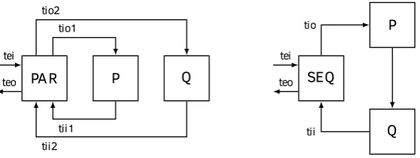
When translating the CSP structures to an FPGA, the order of execution of the operations has to be preserved. In one application of CSP to FPGAs, this behaviour was preserved by creating a dataﬂow model for the synchronisation of processes (Kuipers, ):

The sequential and parallel structure data flow diagrams are shown in [figure .6]. The sequential operation is achieved by pipelining processes. When a sequential block receives a token, the token is forwarded to process P thereby activ-ating it. When process P is finished it forwards the token to the next process in sequence, process Q. Finally, the last process returns its token to the sequential structure. The sequential structure then returns its token to its parent.

The parallel operator produces as much tokens as the amount of processes in parallel. This way all processes are activated simultaneously. After all processes in parallel have ﬁnished the parallel structure returns its token. This means the parallel structure has to collect all the tokens and return its own token only when all internal tokens are received.

Figure .6:Data ﬂow graphs of the par-allel and sequential composition. Lines carry tokens. Processes are denoted as boxes (Kuipers, ).

Channels become bi-directional synchronous communication channels (Kuipers, ):

[image:17.595.65.371.510.625.2]

(18)

va

δ γ π

Figure . :Dataﬂow task with a con-sumption ofγon the incoming edge, and a production ofπon the outgoing edge. The incoming edge hasδinitial tokens.

vb

5 3

Figure .8:An SDF task with a self-loop in order to limit parallel execution. The consumption and production on the self-loop is .

vc

Figure . :An HSDF task. The con-sumption and production on the incom-ing and outgoincom-ing edges is .

.

Synchronous dataﬂow

Dataflow is a way of modelling systems by describing the operations of a stream of data, usually expressed via dataflow diagrams. The dataflow model is closely related to the Kahn Process Network (KPN) model (Lee and Parks, ). Dataflow is used for the design, analysis and optimisation of concurrent real-time systems, and data processing applications (M. Bekooij et al., ).

Dataflow diagrams—such as the one shown in figure . —are expressed in terms ofactors(also known astasks) often indicated byv(figure . ). Actors perform an action taking a constant firing duration (ρ), edges (also known asqueues) that represent buffered unbounded commu-nication channels andtokensthat represent a model of data in such a channel. Actors require a fixed number of tokens on all incoming edges before they can be executed (γ), and produce a fixed number of tokens on all outgoing edges (π). Edges can contain initial tokens (in-dicated by a dot and/orδ). No explicit value forπ,γandδmeans the corresponding value is . A cyclic dependency of a number of actors is called acycle.

An actor can be executed multiple times in parallel, as long as a sufﬁ-cient amount of tokens is available on all edges. The parallel execution of a task can be limited by adding an edge from the task to itself—a self-loop—with an initial token (ﬁgure .8). This limits the parallel execution of the task by creating a dependency on the previous execution of the task.

Synchronous dataflow (SDF) is a variant where the number of data samples that are produced and consumed is specified beforehand (Lee and Messerschmitt, 8 ). Synchronous data flow allows algebraic analysis of real-time properties, including deadlock freedom, and peri-odic behaviour.

Homogeneoussynchronous dataﬂow (HSDF) is a subset of SDF where the number of tokens produced and consumed by a task is always one (ﬁgure . ). HSDF is easier to analyse than SDF, but less express-ive. SDF models can, however, be converted into an HSDF model (M. Bekooij et al., , p. 8 ).

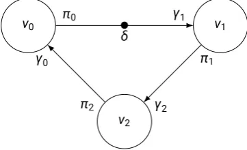
v0

v2

v1

π0 γ1

δ

π1

γ2 π2

[image:18.595.123.304.528.638.2]

γ0

Figure . :Example of an SDF dia-gram (based on M. Bekooij et al. ( )) containing three actors, (v0,

v1,v2) and production (π), consumption

(γ) and initial tokens (δ) indicated.

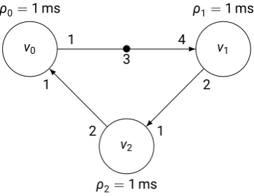
Figure . shows the example SDF diagram from ﬁgure . with con-crete values for the production and consumption of tokens on the edges, and the ﬁring duration for each actor indicated. This diagram has three actors (v1,v2andv3) and three edges.

(19)

v0 ρ0=1 ms

v2

ρ2=1 ms

v1 ρ1=1 ms

1 4

3

2

1 2

1

Figure . :SDF diagram in ﬁgure .

with ﬁring durations indicated (ρ) and values for production, consumption and initial tokens ﬁlled in.

The graph, however, is notdeadlock free: there are not enough initial tokens in the cycle (consisting of all tasks) to allow any actor to ﬁre.

(H)SDF diagrams allow modelling of both concurrency—using parallelism— and task dependencies—using edges and production of tokens. This applies equally to software and hardware applications, as long as a system ispredictable(M. Bekooij et al., ). Not every system is predictable: a hardware system that depends on non-regular input is not predicable, for example. Unpredictable systems cannot be mod-elled accurately. This is especially true for software running on general purpose processors: delays may be incurred when a memory cache is missed, or a task is preempted by the operating system. In software, therefore, theworst case execution timeis used, which can be estim-ated from a statistical set of execution times.

.

Overview

Table . shows the analysability of the modelling techniques com-pared in the previous sections with respect to the following items to analyse:

• Data dependency: the dependencies of tasks with regards to the data they process. Does the diagram express that A should al-ways be applied before B?

• Deadlock: is it possible for the system to be blocked, or stops ex-ecuting, because of mutual data dependencies or other reasons? If a deadlock occurs a control system will halt completely.

• Livelock: is it possible for the system to be stopped because one item does not stop executing? If a livelock occurs the control system will seem to halt while the internal processes keep ex-ecuting.

• Scheduling: is it possible to create a schedule for the execution of operations for tasks? Is it possible to check if a system can, in fact, be scheduled? This information is important for estimating if the system can be deployed on the target system. Without a schedule it is impossible to know if all tasks can be executed and what the input/output latency is.

[image:19.595.122.307.72.214.2]

(20)

• Throughput: can the throughput (i.e. data samples per second) of the model be calculated? The throughput puts an upper bound on the performance of the system. If this upper bound is too low for the needs of the control engineer, either the platform or the design need to be changed.

• I/O latency: can the latency between the inputs and outputs of the system be determined from the model? High I/O latency will interfere with the execution of the control system.

Analysis

Block

Diagram CSP (H)SDF

Data dependency ✓ ✓ ✓

Deadlock – ✓ ✓

Livelock – ✓ –

Scheduling – ✓ ✓

Resource contention – ✓ ✓

Throughput – ✓ ✓

Latency – – ✓

Table . :Comparison of examined modelling methods.

(H)SDF tasks always ﬁnish executing making livelock impossible.

Timed CSP only (Oguz, Broenink and Mader, ).

Needs to be explicitly modelled. Prob-abilistic contention is complex (Kumar et al., ).

Complex (Woodside, 8 )

.

Choice of modelling technique

The chosen modelling technique needs to:

• Allow analysis of the feasibility of the system: is the system valid, does it perform the required functionality, does it contain dead-locks, etc.

• Allow analysis of the schedulability of the system. This allows insight into the question whether all the tasks that need to be performed can be performed in the available computing time.

• Allow analysis of the timing and delays. This allows insight into the delay between incoming and outgoing samples, and which operations cause the most delay.

• Allow translation into an optimal software solution.

• Allow translation into an optimal FPGA solution.

Requirement

Block

Diagram CSP (H)SDF

Feasibility − + +

Schedulability − − +

Timing/delays − − +

Software app. ± + +

FPGA app. ± ± +

Table . :Evaluation of the suitability of block diagrams CSP and (H)SDF.

Table . shows an evaluation of the suitability of block diagrams, CSP and (H)SDF as modelling methods for the analysis and simulation of a system. The suitability for a requirement is rated on a scale consisting of−(unsuited),±(somewhat suited), and+(well-suited). Reasons for the ratings are as follows:

[image:20.595.102.328.185.302.2] [image:20.595.117.315.541.634.2]

(21)

Automated analysis and simulation of control systems using dataﬂow Chapter . Modelling techniques 6

A

1 1

Figure . :Example representation of the equivalent of ablockin HSDF.

A

10 1

Figure . :Example SDF representa-tion of downsampling with a factor .

information, no schedule can be constructed and no delays de-termined. Block diagrams, being a series of operations on a sig-nal, can be converted into software relatively easy. The resulting software, however, is not necessarily optimal. It is somewhat unsuited to a hardware application though, as there is no inform-ation about the execution time of operinform-ations. This means that there is no easy way to create a performant, well-synchronized system that conforms to the equations.

• CSPdoes allow insight into the validity of the model in the form of deadlock and livelock freedom. Constructing a schedule is somewhat more complex, but possible (Oguz, Broenink and Mader,

). Calculating the timing and delays may be possible from this schedule, but requires new research into this area. CSP, how-ever, is especially suited to developing concurrent software, this being itsraison d’être. There exists previous research, however, that shows that applying CSP to hardware does not necessarily lead to an efﬁcient implementation (Kuipers, ).

• HSDF and SDFdo allow insight into the deadlock-freedom of a model, and itsconsistency. SDF, being a more expressive form of dataflow, is slightly less easy to analyse. From a consistent model a self-timed schedule can be determined. Timing informa-tion is an explicit part of a dataflow model. Engineering software and hardware with dataflow models is also relatively straight for-ward.

Dataflow in the form of SDF or HSDF is more suitable than CSP for the (static) analysis of a platform-specific model, and is better suited for modelling hardware targets. Block diagrams are entirely unsuitable for analysis platform-specific models. However, as control engineers tend to model in block diagrams—block diagramsaremore suitable for control theory—a model-to-model conversion from block diagrams to SDF will allow a ‘best of both worlds’ approach: control engineers can work with modelling methods that are suitable for their domain, while the real-time analysis and synthesis is performed using methods more suitable for real-time analysis.

In section . it was explained that a more expressive model usually leads to a model that is harder to analyse. This is also the case for SDF over HSDF: themaximum cycle ratio(MCR) of an HSDF diagram can be calculated with a polynomial algorithm, but this is not the case for SDF diagrams (M. Bekooij et al., , p. ). It would therefore be beneﬁ-cial to limit the modelling technique to HSDF in order to maintain the most analysable model possible. For almost all equivalent elements in a block diagram, this is possible: a mathematical operation usually does not operate in a way where it consumes multiple values from the same input at once. Such mathematical operations can therefore be represented by an HSDF task (ﬁgure . ).

The main exception to this is resampling: as every sample is repres-ented by a token in an SDF-model, an SDF task equivalent needs to consume and produce tokens in a ratio equal to the resampling ratio (figure . ). Resampling elements are sometimes explicitly defined in models, but can also be required when having a system with dif-ferent sampling frequency domains that communicate between these domains. This means that the modelling technique has to be SDF, but HSDF analysis techniques can be applied as long as there are no re-sampling elements involved or the rere-sampling elements are converted to HSDF first.

(22)

(23)

8

Chapter

Model-to-model conversion

Because of the beneﬁts of allowing control engineers to create platform-independent models in block diagrams, but creating the platform-speciﬁc model in SDF (see section . ), it is required to perform a model-to-modelconversion from block diagrams to SDF.

.

Procedure

The procedure for translating a block diagram into SDF is as follows:

. Ensure all elements in a diagram are deﬁned. If the input and outputs of the system are not deﬁned (but only marked asu(t), for example), the system cannot be fully analysed.

. Convert all blocks and points to tasks:

• Blocks operate on a single input and have a single output (e.g. integrator).

• Points have multiple inputs and a single output (e.g. sum-ming point), or vice versa (e.g. take-off point). Because tasks consume and produce on all edges the former sume multiple tokens and produce one, and the latter con-sume a single token and produce multiple.

Keep the connecting arrows asedges.

. Add a self-edge to elements that cannot be executed multiple times in parallel with itself (e.g. sampling input). This also ap-plies to tasks that operate on an internal variable (like integration elements) to avoid race conditions: the token on this self-edge represents the state of the internal variables of the task.

. Add initial tokens to edges that require initial values. This in-cludes all self-edges, but also one token per feedback loop.

(24)

Automated analysis and simulation of control systems using dataﬂow Chapter . Model-to-model conversion

.

Example

Figure . shows an example block diagram. The following steps are taken to convert this model:

. The input and output signals,u(t),x(0)andy(t), are converted to explicitsourceandsinkelements (ﬁgure . ).

. All blocks and points are converted to tasks (ﬁgure . ). . Thesources(u(t),x(0)) are given a self-edge (ﬁgure . ). . Initial tokens are given to the self-edges and the output of the

integration task (ﬁgure . ).

. Execution times from the task types, ﬁctional in this example, are added to the diagram (ﬁgure .6).

This model is a valid HSDF model (because all tasks produce and con-sume one token), and can therefore be fully analysed.

B ´ C

A D

u(t) +

+

y(t) +

+

Figure . :Example of a block diagram. Adapted fromControl Systems/Block Diagrams( 8).

u(t) B ´ C y(t)

A D

+

+ +

+

Figure . :Block diagram of ﬁgure .

[image:24.595.83.350.286.483.2]

(25)

u(t) n1 B Σ1

´

n2 C Σ2 y(t)

A D

Figure . :SDF diagram created from ﬁgure . by converting elements to tasks.

u(t) n1 B Σ1 ´ n2 C Σ2 y(t)

A

D Figure . :with self-loops.SDF diagram of ﬁgure .

u(t) n1 B Σ1

´

n2 C Σ2 y(t)

A D

Figure . :SDF diagram of ﬁgure .

with initial tokens.

u(t)

ρ=10 ms n1

ρ=1 ms

B

ρ=10 ms

Σ1

ρ=2 ms ´

ρ=10 ms n2

ρ=1 ms

C

ρ=5 ms

Σ2

ρ=2 ms y(t)

ρ=1 ms

A

ρ=3 ms

D

ρ=12 ms Figure .6:SDF diagram of ﬁgure .

[image:25.595.73.471.90.735.2]

(26)

.

Example of performed analysis

The model in ﬁgure .6can be analysed by standard HSDF methods. First the validity of the model is analysed. This is simply checking if all edges are connected, ergo: the model isvalid.

Mathematically, a connected and consistent model is guaranteed to have topology matrix (Ψ) with a rank one less than the amount of tasks in the graph (|V|) (M. Bekooij et al., , p. ). This always holds true for an HSDF graph, which the diagram in ﬁgure .6is.

A deadlock will occur when there is a cycle without initial tokens. The cycles in ﬁgure .6are:(u(t)),(´), and(Σ1,

´ ,n2,A

)

. All of these cycles contain an initial token, meaning the model contains no deadlock.

Themaximum cycle ratio(MCR, μ) for graphG(being an HSDF dia-gram), with cyclesC(G), tasksV(G)and edgesE(G)can be calculated with the following equation (M. Bekooij et al., , p. ):

μ(G) = max

c∈C(G) ∑

v∈V(c)ρv ∑

e∈E(c)δv

( . )

This ﬁnds that thecritical cycleof the system is(Σ1, ´

,n2,A

)

with an MCR of 6 ms. This represents theminimum period in the periodic schedule for this system. In this diagram this means that the control system should not have a higher sampling rate than 1

16 ms: because

in-putsu(t)andx(0)have a ﬁring duration that is lower (ergo: a frequency that is higher), the number of tokens onsomeedge will grow exponen-tially.

By calculating the start-times of the actors in the SDF diagram, the input/output-delay can be calculated. This is straightforward in the case of the diagram in ﬁgure .6: assumingu(t)starts att = 0 ms, the ﬁnish time ofy(t)ist=42 ms (the sum of all tasks in the longest path between input and output). This should be smaller than a single sample period as well, making the minimum sampling period ms, equivalent to a maximum sampling frequency of approximately .8 Hz.

(27)

Chapter

Tool design

The technique for converting a block diagram is embedded into a proof-of-concept tool with the ability to perform static analysis and simula-tion. This allows control engineers to make use of the added insight provided by the model conversion to dataﬂow. The proof-of-concept tool is implemented using Python.

.

Functionality

In order to attain the goals set out in section . , the tool should have the following functionality:

• Have an annotated explicit block diagram as input.

• Have a standardised system of annotations that include all in-formation required for modelling and simulation.

• Be able to convert the given model into a dataﬂow (SDF) model automatically.

• Be able to perform static analysis on the real-time properties of the model.

• Be able to give clear feedback on the result of the analysis.

• Be able to simulate the real-time behaviour of the model.

• Be able to perform run-time sanity checks during the simulation.

This can be combined with the “ Cs” (section . . ) to separate the components of the tool into the the following, modular, parts:

• Aconﬁguration ﬁlecontaining information provided by the con-trol engineer: the blocks in the diagram with their types, para-meters and connections, and the target platforms for the control system.

• Acomponent librarycontaining task abstractions and implement-ations of elements in the block diagram.

• Thecore librarycontaining everything for creating and analysing the model.

(28)

Automated analysis and simulation of control systems using dataﬂow Chapter . Tool design

name: test

platforms:

raspberry_pi: default: true clock_speed: 1 GHz nucleo_f411re: clock_speed: 100 MHz model: task_1: ... task_2: ...

Listing . :Example conﬁguration for a model.

models from the core allows the range of available components to be extended without inﬂuencing core functionality.

.

Model representation

The representation of amodelis composed of a set oftasks connec-ted byedges. This representation is close to the SDF deﬁnition of the model, but extended by the properties required for simulation. Fig-ure . shows an SDF model similar to the one from ﬁgure . as mod-elled by the tool.

v1

ρ=1000.0 µs

v2

ρ=1000.0 µs

ﬂoat641

1 v0

ρ=1000.0 µs

ﬂoat64 1 1 ﬂoat64 1 1

Figure . :SDF model based on ﬁg-ure . as modelled by the tool. The production and consumption of tasks is indicated on the beginning and end of the edges. The type and number of ini-tial tokens on edges (δ, omitted if zero) are indicated in the middle of the edges.

The inputs and outputs of tasks are not explicitly modelled as separate components, but instead kept in a list within the task itself. This allows tasks to communicate via these inputs and outputs, without having to add additional logic for interfacing inputs and outputs with the corres-ponding tasks and edges.

. .

Model

The conﬁguration contains three top-level sections:

• namecontains a unique identiﬁer for the model.

• platformconfiguration that configures what platforms the sys-tem is deployed to, and what the settings of this platform are. This configuration allows for more accurate estimation of the performance of a certain component based on the platform.

• modelconfiguration that contains the definitions and configura-tion for the defined elements of the model (thetasks), and how they are connected.

In the example shown in listing . , the name of the model is ‘test’. Tasks will be analysed as if they run on a Raspberry Pi clocked at GHz by default. The model contains two tasks.

. .

Task

A task is the representation of an SDF actor containing all information required for static analysis, and simulation.

A task is speciﬁed with the following required information:

• Anameused for identiﬁcation of the task.

• Atypethat determines the implementation of the task. • Parametersthat conﬁgure this task.

• Where theoutputsof the task connect to.

[image:28.595.79.354.216.305.2]

(29)

pid_1:

type: pid

platform: raspberry_pi params:

kp: 1 ti: 10 td: 0.5 outputs:

out: dac.in

Listing . :Conﬁguration for a PID element.

Allelementsare implemented as extensions of a basictaskin the com-ponent library. This allows a few common parameters to be set, mainly

WCET(equivalent to the ﬁring duration), and value logging conﬁgura-tion. This basic task is part of thecoreof the tool, allowing elements to be created with minimal effort.

Listing . shows an example of the configuration for a PID element. The name of the element is determined by the key (pid_1) of this con-figuration, the type ispid. The PID element is configured with para-metersKp=1,Ti=10 andTd=0.5. The output of the PID controller

is connected to the input ‘in’ of the task named ‘dac’.

. .

Edges, tokens and types

Anedgeis modelled as a typed unbounded FIFO containing tokens. Having unbounded capacity is sufﬁcient for the simulation purposes. Because a consistent SDF graph will have a limited number of tokens on any edge, this amount can be constraint for the synthesis. The edge is created in the source task and then connected to the destination task when the model is created, allowing only the output connections to be speciﬁed. Edges perform a type check when a token is added to the the edge, in order to detect programming or design errors.

Tokens are simple objects containing a data type, an inception time and a value. The token performs active conversion of the value on its creation in order to model behaviour like quantization. The inception time can be used to see the lifetime of tokens but also, more import-antly, to calculate the start time of tasks.

How a value is converted is modelled by thedata typethat contains a type name, and parameters noting its properties—like the number of bits and if the data type is numeric. These properties allow tasks to change their execution model in order to better reﬂect reality: perform-ing an operation on a thousand bits is often slower than performperform-ing it on eight.

. .

Platform

Platforms contain the properties of a hardware platform. This is cur-rently limited to theclock speedof the platform, but can be expanded to contain information about properties like the availability of floating point units, performance of specific operations (e.g. multiplication and addition), word size, and available inputs and outputs of the platform. This could also influence the type that a task uses for its calculations: a -bit floating point value on a -bit platform, but a 6 -bit floating point value on a 6 -bit platform, for example.

.

Simulation method

Existing simulation solutions for SDF, like HAPI (Kurtin, Hausmans and M. J. Bekooij, 6), are mainly focussed on the activation of tasks and the resulting schedule. While this gives a good indication of the per-formance of a system modelled by SDF, this contains no information about the values embedded in the tokens.

(30)

plant

ρ=0.0 µs analog

1

analog,δ=2 1

Figure . :Plant ‘task’ with two initial tokens on the outgoing edge.

• Before a task can be executed, all its incoming edges need to contain at least as many tokens as the task consumes on the respective edges.

• The task runs for a ﬁxed amount of time, after which the task produces a certain amount of tokens on its outgoing edges.

Before simulation all tasks are added to a queue. Tasks in the queue are simulated as follows:

. Check if the task is ready. If not, skip this task to simulate other tasks.

. Consume all tokens and perform operations using the values.

. Produce tokens with the result of the operations. The new tokens have an inception time that is the maximum of the inception times of the incoming tokens.

. Remove this task from the queue if the inception time of the pro-duced tokens is greater than or equal to the simulation stop time. Go back to step otherwise.

This method results in simulation of the target system in a worst-case scenario. The accuracy of the simulation depends on the accuracy of the WCET estimates and the precision of the data types. Because of the software used, the accuracy of both time and simulated values, however, is limited to a double precision ﬂoating point value. No prob-lems are expected because of this limitation.

All tasks have a common parameter named ‘log’ that allows tasks to log values to either a ﬁle, or a plot. This plot is constructed after the simulation is ﬁnished, and contains all output values of the tasks that log measurement data for use in the plot.

. .

Plant representation

Modelling a plant is required for creating an accurate simulation. There are two choices for simulation: (i) co-simulation against simulation software, or (ii) perform the full simulation of the plant within the tool itself. The first option has preference because there is sufficient soft-ware available for simulation, and this can perform simulation of sig-nificantly complex models and the internal dynamics of the plant. Not implementing simulation also has the benefit of keeping the tooling simple and to the point, applying theKISSprinciple (Hanik, 6).

Because interfacing with simulation software brings along its own com-plexity, however, co-simulation has not yet been implemented.

(31)

Automated analysis and simulation of control systems using dataﬂow Chapter . Tool design 6

.

Overview of functionality

A proof-of-concept tool is implemented using the “ Cs” for the struc-ture of the conﬁguration ﬁles and program libraries. The proof-of-concept can perform the following functions:

• Create a representation of an SDF-based platform-specific model based on a configuration file with a platform-independent model and parameters.

• Create a representation of a plant in a limited capacity.

• Perform analysis on this platform-speciﬁc model using the meth-ods described in section . .

(32)

Chapter 6

Execution

The following sections show some analysis of simple control systems and how analysis can be performed on them. All conﬁguration for the models discussed can be found in appendixA.

6. SDF validity

To check if the SDF properties are correctly analysed, several examples from M. Bekooij et al. ( ) have been modelled as test cases. The deﬁnitions of these test cases can be found in appendixA. . For each case the following happens when checking the model with the developed tool:

v0

ρ=1000.0 µs

generic, δ=1 1 1

v1

ρ=1000.0 µs

ﬂoat64 1

1

v2

ρ=1000.0 µs ﬂ_{oat64 1}

1 ﬂoat641

2

Figure 6. :Example of an inconsistent model, adapted from M. Bekooij et al. ( ).

↑2

+

−

Figure 6. :Example of a block diagram that can result in the situation in ﬁg-ure6..

Figure6. shows a model that is notconsistent: the number of tokens on the edges do not return to the initial state after a certain number of executions. This can be caused, for example, by connecting a signal before upsampling to the signal after upsampling (ﬁgure6. ). The tool gives the following result:

Result: model is not consistent

[image:32.595.93.334.422.601.2]

(33)

Automated analysis and simulation of control systems using dataﬂow Chapter 6. Execution 8

v0

ρ=1000.0 µs _2int64,int64 3_δ₌₃ ρ=1000.0 µsv1

2

3

Figure 6. :Example of a consistent model with deadlock, adapted from M. Bekooij et al. ( ).

Figure6. shows a model that is consistent but contains a deadlock because of insufﬁcient tokens available on the edge fromv1tov0. This

results in the following output:

Result: model is not deadlock free

Stopping analysis because of problems with the model

v1

ρ=1000.0 µs

v2

ρ=1000.0 µs

ﬂoat641

1 v0

ρ=1000.0 µs

ﬂoat64 1

1

ﬂoat64 1 1

Figure 6. :Example of a consistent model with deadlock, adapted from M. Bekooij et al. ( ).

B(s)

C(s)

A(s)

Figure 6. :Example of a block diagram that leads to the situation in6. .

Figure6. , used as example SDF graph in earlier chapters, shows an-other model that is consistent but contains a deadlock. This deadlock is caused by a circular dependency without initial tokens. Depending on the exact type of blocks, this situation may arise in a block diagram with such a circular dependency (ﬁgure6. ). This, once again, results in the following output:

Result: model is not deadlock free

Stopping analysis because of problems with the model.

Figure6.6shows a model that is consistent and deadlock free because there are sufﬁcient initial tokens on the edge fromv1 to v0 to allow

execution. The result is shown below. Note that the slowest internal loop reﬂects the inverse of the throughput.

Result: model is valid

Slowest internal loop is 0.5 ms (tasks: ['v0', 'v1'])

Figure6. shows another model that is consistent and deadlock free. This results in the following output:

Result: model is valid

[image:33.595.143.289.72.120.2] [image:33.595.96.333.235.407.2]

(34)

Automated analysis and simulation of control systems using dataﬂow Chapter 6. Execution

v0

ρ=1000.0 µs _2int64,int64 3_δ₌₄ ρ=1000.0 µsv1

2

3

Figure 6.6:Example of a consistent model and deadlock-free model, adap-ted from M. Bekooij et al. ( ).

v0

ρ=1000.0 µs

generic, δ=1 1 1

v1

ρ=1000.0 µs

ﬂoat64 4

1

v2

ρ=1000.0 µs ﬂ_{oat64 2}

1 ﬂoat642

1

[image:34.595.97.338.541.635.2]

(35)

[image:35.595.416.505.87.118.2]

ADC

Figure 6.8:Block diagram for the sys-tem simulated in ﬁgure6. .

ADC

ρ=T

[image:35.595.93.340.231.426.2]

sin(2πt)

Figure 6. :Example of an incorrectly modelled ADC task with a sine wave input.

ADC sin

ρ=T

Figure 6. :Model of a sine wave in-put/ADC combination that models a sine wave input and an ADC in a single task.

ADC

ρ=T

sin(2π(t+T−τ))

Figure 6. :Single task model where the values produced by the plant com-pensate for the ADC delay.

ADC

ρ=τ

ADC

ρ=T

sin(2π(t+T))

Figure 6. :Single task model where the values produced by the plant com-pensate for the ADC delay.

6. Quantization and delay

An ADC is a more complex component to model: it should produce tokens at a certain sampling rate (fs). But a realistic ADC also produces

the measured values with a certain sampling delay (τd).

Figure6. shows the result of simulations of an incoming Hz sine sig-nal and the digital value produced by both an ideal ADC with zero delay, and a slow ADC that requires ms to process a sample. The corres-ponding block diagram is shown in ﬁgure6.8. While the quantization is apparent in both ADC signals, only the slow ADC introduces a delay as well. This example shows that an incoming signal is distorted in the same way that one would expect to happen in reality.

Figure 6. :Simulation showing un-delayed sampling (blue) and un-delayed sampling (orange) of an incoming sig-nal (green).

This is not trivial to reproduce in SDF. Simply converting the ADC to a single HSDF task with a self-edge and a sine input (ﬁgure6. ) leads to an inaccurate model: if the task has a ﬁring duration of a single sampling period (T) all tokens produced by the ADC task will have delay of a full sampling period. There are three ways of resolving this:

. Model the setup as an input that combines the sine wave and ADC (ﬁgure6. ). In this case the produced tokens should con-tain a value that takes into account the sampling delay (τd): a

token produced attcontains the quantized value of sin(2π(t−τd)).

Although this is the correct model of the system, it requires that the ADC task has knowledge about the real-world, and that the real-world is not modelled in dataﬂow.

. Take the behaviour of the ADC into account when modelling the plant, and manipulate the tokens so the timestamps stay realistic (figure6. ). This can only be valid when the plant has no influ-ence on the dataflow representation of the system, and requires knowledge of the ADC in the plant.

. Have the plant output lead by a single sampling period, and model the ADC as two tasks (ﬁgure6. ). This is similar to the third solution, but requires no knowledge of the ADC in the plant.

(36)

6. PID controller

set-point PID DAC plant

ADC

r(t) + e(t) ud(t) ua(t)

ya(t) yd(t)

[image:36.595.106.322.98.176.2] [image:36.595.65.463.251.386.2]

−

Figure 6. :Example block diagram for a PID controller.

Figure6. shows an example of a PID controller. As per the workﬂow in section . , all elements of the block diagram have been made ex-plicit: the block diagram contains a digital to analog converter (DAC), a analog to digital converter (ADC) and an explicit setpoint source.

adc

ρ=1.0 µs

generic, δ=1 1 1

sum

ρ=20.0 µs

uint8

1

1 _plant

ρ=0.0 µs

analog, δ=1

1 ₁

setpoint

ρ=1.0 µs

generic, δ=1 1 1

ﬂoat641 1

pid

ρ=1000.0 µs

generic, δ=1 1 1

dac

ρ=10.0 µs

ﬂoat641 1 ﬂoat641

1 generic, δ=1

1 1

analog1

1 generic, δ=1

1 1

Figure 6. :SDF equivalent of the con-troller shown in ﬁgure6. .

Creating a configuration for this model (see appendixA. ) results in the SDF diagram in figure6. . The configuration for this model is straight-forward, with the following observations:

• For this example, none of the components have been set to be executed in parallel in order to simplify manual analysis of the model—all tasks are executed in sequence.

• The setpoint has a sample rate set identical to the ADCs sample rate in order to ensure that the time of production of the setpoint matches the time of production of the samples.

• In the model shown, the ADC is set to an extremely high sampling frequency ( MHz) in order to observe what the tool has to say about the rest of the system. With such a high sampling fre-quency, the ADC will not be the limiting factor of the system, which it should be.

• Without changing the sampling frequency, thePIDelement is the slowest element with an execution time of ms. This means that the minimum sampling frequency for a working system is kHz, which is used in the simulation.

Figure6. 6shows a plot of the setpoint and ADC signals in ‘ideal’ con-ditions: the PID-controller has a ﬁring duration of seconds (i.e. the calculations takezerotime) in order to minimize the input/output delay, and ADC and DAC can deliver perfect analog signals. While the over-shoot of the controller is large, the plant reaches the setpoint value in approximately ms. Note that the delay of components other than the PID and ADC tasks is still present. This adds up to an input/out-put delay of µs (caused by thesumanddactasks), or . % of the sampling interval.

(37)

0.0

0.1

0.2

0.3

0.4

0.5 time (s)

0

2

4

6

8

10

12

14 va

lue

adc_out

adc_self

plant_0

setpoint_0

Figure 6. 6:Plot of the performance of the PID controller in ideal conditions.

0.0

0.1

0.2

0.3

0.4

0.5 time (s)

0.0

2.5

5.0

7.5

10.0

12.5

15.0

17.5 va

lue

[image:37.595.67.365.74.548.2]

adc_out

adc_self

setpoint_0

plant_0

Figure 6. :Plot of the performance of the PID controller with discrete ADC/-DAC values.

and DAC output discrete values. The performance of the controller is affected, now reaching the setpoint after approximately ms.

Figure6. 8shows a plot of the same controller, but now with the ﬁring duration of the PID controller restored to its original value. The addi-tional delay between the input and output has caused the controller to no longer be stable. The total input/output delay is now . ms, or

(38)

0.0

0.1

0.2

0.3

0.4

0.5 time (s)

0.0

2.5

5.0

7.5

10.0

12.5

15.0

17.5

20.0 va

lue

adc_out

adc_self

plant_0

setpoint_0

[image:38.595.66.365.313.534.2]

Automated analysis and simulation of control systems using dataflow