University of Twente
Deparment Applied Mathematics
Chair Hybrid Systems
Robust sensor coverage in a
two-dimensional area
Candidate:
Floris
Broekema
Supervisor:
P.
Frasca
Preface
This report describes a master thesis about robust sensor coverage. The assignment is done within the University of Twente at the chair hybrid systems, of the department mathematics. The time assigned to this thesis is about 32 weeks, which is equal to 40 European credits. The supervisor of this master thesis is Paolo Frasca, working at the chair hybrid systems. Among other subjects he has done research in the fields of hybrid systems, system control, opinion dynamics and robust sensor coverage in a 1-dimensional space.
Within this master thesis, the task is to find a good or even optimal deployment of sensors in a 2-dimensional space. Besides that, the sensors can fail with a certain probability which means that the solution must be robust, such that it takes the possible failures into account. Various proper-ties are known for the 1-dimensional space, the intention is to extent this to a 2-dimensional space.
Abstract
Contents
1 Introduction 4
1 Problem description . . . 4 2 Former research . . . 5
2 Model 7
1 Mathematical problem description . . . 7 2 Geometrical properties of the cost function . . . 8
3 Grid and random uniform deployment 11
1 Defining the deployment strategies . . . 11 2 Non optimality of the grid . . . 12 3 Simulation results . . . 13
4 Cost analysis 17
1 A general lower bound . . . 17 2 Known theorems about sensor coverage . . . 18 3 Comparison with simulations . . . 21
5 Sensors deployment algorithms 24
1 Gradient descent algorithm . . . 24 2 Gradient based algorithm . . . 31
6 Discussion 34
7 Conclusion 36
Chapter 1
Introduction
1
Problem description
This master thesis is about robust sensor coverage in a two-dimensional space. Sensor coverage means that an area (in this case a two-dimensional area) must be filled with sensors such that the sensors can get information from the whole area. Possibly, the sensors only have a certain sensing radius which can be seen as a disk around the sensor in which the sensor can measure. Sensor coverage is important for many systems, for example a smoke detection system. In a smoke detection system the whole building must be covered with sensors such that smoke is detected as fast as possible. In researches on sensor coverage, there are two different aims, namely to use the least amount of sensors to cover the whole area, or to use a fixed number of sensors to cover the area as good as possible. In this research the aim is to maximize the quality of the sensor network and to find the best sensor covering with a fixed number of sensors.
The quality of a sensor deployment can be measured in various ways. Central in these measures is the distance from a point in the area to the closest sensor. In this report the euclidean distance will be used to determine the distance from the sensors to any point in the area. The quality of a sensor network will be defined as the (weighted) average distance of each point of the area to the closest sensor. However, in this research the quality of a sensor network is defined as the distance to the worst detectable point. Throughout this report, the quality of a sensor deployment is called the cost of the sensor deployment. In other words, the cost is the maximal distance from any point in the area to the closest sensor. This measure relies on the worst case scenario. To restrict the problem and to avoid assumptions on the cost definition, only a convex area will be considered, namely the unit square area. Most findings can be adapted to other convex areas but this will not be done within this research.
In chapter 2 of this research the general problem statement and details about the cost computation will be given. Properties of the cost function will be derived which are important to understand the behavior of the cost function and these will be used later on in this report. In chapter 3, two deployment strategies, namely the random uniform and the grid deployment, will be defined and discussed. Cost simulations will be done and the strategies will be compared. Besides that, the two deployment strategies will be used throughout the report for theorems and simulations. Furthermore, known relations between the cost of a sensor deployment, the number of sensors and the probability on active sensors will be analyzed and a general lower bound will be constructed in chapter 4. With this lower bound, a minimal cost can be deduced for all sensor deployments. This lower bound will be compared to known asymptotic relations on the sensing radius which only hold when the number of sensors goes to infinity. In chapter 5 two deployment algorithms will be defined which aim to find optimal sensor locations which minimize the cost. One of these algorithms will be the gradient descent algorithm and the other is derived from the gradient descent algorithm. Simulations are done for both the algorithms and the critical points and the convergence will be analyzed. Then the results of the whole research will be concluded and discussed. At last recommendations for further study are presented.
2
Former research
Much research has been done on sensor coverage problems. In this research the sensors are as-sumed to have fixed locations, but in other researches the sensors can be dynamic and have to move through an area. Some examples of studies that are related to this study are: a book which discusses most sensor coverage problems in general [1]; papers on algorithms for making good sensor deployments [2][3]; papers on dynamical coverage problems with restricted communication radius [4] and papers on analyzes of the asymptotic relations between the number of sensors and the minimal radius needed for coverage [5][6]. Below a short description of several researches are given and is described how they are used in this research.
The problem of robust sensor coverage has also been studied in the one-dimensional setting [7]. This research considers the same kind of assumptions such as stationary sensors, the probabilistic sensor failures and the same cost function. The sole difference is the dimension in which the sensors are deployed. consequently, the same methods are considered and if possible extended to the two-dimensional case. In one dimension, the problem can be described as a linear program and then be solved. Furthermore, in this research ([7]) an equispaced sensor deployment is defined and analyzed for its cost and relative cost to the optimal solution. Besides that, the asymptotic relations are examined together with the performance of a random uniform deployment.
Chapter 2
Model
In this chapter the mathematical problem description will be defined and explained. First the variables will be defined such that a cost function can be made. Then the cost function will be explained and described with more detail. This is done to improve understanding of how the cost behaves for different sensor deployments.
1
Mathematical problem description
In this section the general problem will be described with a mathematical model. Let Q be a convex two-dimensional space on which sensors are deployed. For simplicity, letQbe the square unit surface, [0,1]×[0,1]. On this arean >0 sensors must be deployed. Let the locations of the sensors be xi, i= 1,2,...,n. The sensors must be deployed withinQ, so xi ∈Q. Each sensor is
active with probabilitypand not active with probability ¯p= 1−p. The failure events of different sensors are assumed to be independent and identically distributed.
Now we can defineC(xA) as the cost of the sensor deploymentxwhereAis the set active sensors.
This cost is given by the worst case performance which is equal to the distance of the farthest point inQto the closest active sensor. For the distance the 2-norm will be used to calculate the Euclidean distance. Then the cost of an active set sensors is equal to
C(xA) = max
s∈Qmini∈Aks−xik2. (2.1)
To be complete, the cost with no active sensors is defined as the largest distance between two points inQ, which is √2. The set active sensors Acan be any subset of {1,2,..,n}. Now letEA
be the event that that the set active sensors is equal to A. Then the probability that event EA
occurs can be calculated as:
P r(EA) =p|A|(1−p)n−|A|. (2.2)
Now the cost function for the whole sensor deployment can be made where all possible active subsets due to sensor failures are taken into account. This can be done by a weighted sum over all the costs for the different active sets A, multiplied by the probability on eventEA. This way
the total cost function is a weighted average over all events, namely the expected value of the cost of a sensor deployment. With this definition of the cost of a sensor deploymentx, the cost can be computed as follows:
C(x) =E(C(x)) = X
A⊆[n]
Throughout the whole research this is the measure of quality for a sensor deployment. Therefore, finding the sensor locationsxwhich minimize this cost function for a givenpis the main goal of this research. With use of this cost function an objective function can be constructed. Because the cost with no active sensors is not different for different deployments, it is not part of the objective function:
min
x∈Qn
X
A6=∅,A⊆[n]
P r(EA)C(xA) (2.4)
2
Geometrical properties of the cost function
As described in the previous section, a cost function describes the total cost of a sensor deployment with stochastic failures of sensors. In this section the cost of an set active sensors will be described with more detail. Besides that, a method to calculate these cost will be explained. As defined in the previous section, the cost of a set active sensors is
C(xA) = max
s∈Qmini∈Aks−xik2. (2.5)
This formula describes how to calculate the distance from the farthest point to the closest sensor. With help of Voronoi regions (Vi) this formula can be rewritten. But first will be explained
what Voronoi partitions are. Each active sensor has its own Voronoi partition which contains the points ofQ which are the closest to that sensor. So a Voronoi region of a sensor depends on the neighboring sensors and is defined as
Vi=
(
s∈Q| ks−xik2≤ ks−xjk2,∀j∈A ∀i∈A,
∅ ∀i /∈A. (2.6)
In figure 2.1 a Voronoi diagram can be seen for a random deployment with 9 active sensors. As can be seen, the cost is attained at only one point of Q. The cost is defined by the point which is the farthest away from the closest sensor. This is the same as calculating the farthest point in each Voronoi regioni to the corresponding sensori and then maximizing over all active sensors. This because the points in the Voronoi partition of sensori solely contains the points which are the closest to sensori. Now the cost function can be rewritten as:
C(xA) = max i∈A maxs∈Vi
ks−xik2. (2.7)
This formula can even be made more precise. From figure 2.1 it is clear that the points in a Voronoi partition which are the farthest away from the corresponding sensor, are the points on the boundaries of the Voronoi regions. Let δVi be the edge of the Voronoi partition, then the
formula can be rewritten as:
C(xA) = max i∈A smax∈δVi
ks−xik2 (2.8)
However, not all points on the edge of a Voronoi partition are points on which the maximum distance to the closest sensor can be obtained. Let W be the set of points at which the cost is attained:
W =
a|max
i∈A smax∈δVi
ks−xik2=ka−xik2,∀s∈Q
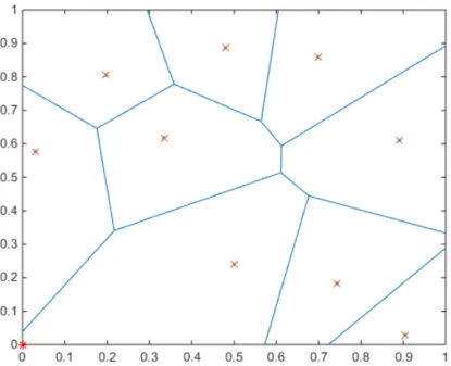
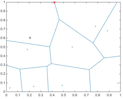
Figure 2.1: A figure of Voronoi partitions created in Matlab for a random deployment in the unit square surface. The red crosses are the sensors and the blue lines are the boundaries of the Voronoi partitions. The cost is attained at the red star at(0,0) and is equal to 0.5546.
Proposition 2.1. The setW can be described as a subset of the union of 3 types of points, namely the vertices of the Voronoi diagram (W1), the points at which the edges of the Voronoi partitions
intersect with the edges ofQ(W2) and the vertices ofQ(W3).
W ⊆W1∪W2∪W3 (2.10)
Moreover, these 3 types of points determine the cost of a sensor deployment.
Proof. First will be explained why the maximal distance to the closest sensor can be obtained by the points of W2 and W3. Consider a sensor with an edge of Qin its Voronoi partition. Then
there is a point on the edge of Qin the Voronoi diagram which has the smallest distance to the corresponding sensor. This point is obtained by moving in a straight horizontal or vertical direc-tion until the edge of Q is reached. From this point, moving along the edge of Q will increase the distance to the sensor (Pythagoras) and this can be done until the Voronoi diagram will be exceeded. The last point before exceeding the Voronoi partition has to be either a corner of Q
or an intersection of the Voronoi boundary with an edge of Q. So this point is inW2 orW3 and
might have the maximal distance to the closest sensor, namely the sensor corresponding with that Voronoi partition.
For the vertices of the Voronoi diagram (W1) a similar argument can be used. Consider two
neighboring sensorsiandj, then for the edge of the Voronoi diagram in between the two sensors we know that the distances to the sensors are equal. Also 1 point, namely the point between the 2 sensors has the smallest distance to the sensors and lies on the edge of the Voronoi partition. Moving along the Voronoi edge from this point will increase the distance to the sensors. This can be done till the end of the Voronoi partition, this point will be either a vertex of the Voronoi diagram or an edge of the areaQ. Here the point on the edge of the areaQis again a point from
W2 and the vertex of the Voronoi partition is inW1.
edges ofQ and the Voronoi partitions and the vertices ofQ. This means thatW is a subset of the union of these points.
Remark 2.1(One-dimensional linear program). In the one-dimensional case it is known that the problem can be written as a linear program. Then the cost is depending on the distances between the sensors and between the begin/end of the interval and the first/last sensor. These relations are linear and thus can be used to write a linear program. In the two-dimensional problem the distances are calculated by the 2-norm which is not linear. Besides that, the points ofW1,W2 andW3 which
determine the cost as described in proposition 2.1 cannot be determined with linear equations either.
Remark 2.2 (Relation to disk-covering problem). When the probability p on active sensors is equal to 1, the cost function as a weighted average over all possible events is reduced to a cost function with only one event. Only the event where all sensors are active is left. Using Voronoi partitions, the objective function can be written as:
C(x) = max
i=1,2,..,nsmax∈δVi
ks−xik2 (2.11)
This function must be minimized to find an optimal deployment in which the sensors cannot fail. This problem is very similar to the disk-covering problem where an area must be covered with circles with a certain radius. The difference is that in the disk-covering problems they increase the number of sensors and in this research, the radius is increased to cover the whole area. How-ever, the solutions are very similar and it can be shown that the optimal solution of the objective function without failure rates is a deployment where the locations of the sensors are the centers of circumcircles of the Voronoi partitions[3]. In other words, circles can be drawn with the sensors as center which passes through all the vertices of the Voronoi partitions.
Now only 3 types of points have to be considered when calculating the cost of a sensor deployment. The cost is defined as the sum over all possible sets active sensors, therefore the number of terms in the sum raises exponentially with respect to the number of sensors. As a result the needed computational time is growing exponential too. To avoid exploding computation time, stochastic simulation will be done such that the number of sensors can be increased. The cost function (2.3) is a weighted sum over all possible events weighted with the probabilities that the events occur. That can be sampled by drawing the set of active sensors from a binomial distribution with chance
pon success. Then the costs can be calculated by computing the distance of each of the points in W1, W2 andW3 to the closest sensor. Then the maximal distance from any of these points to
Chapter 3
Grid and random uniform
deployment
In this section the grid and the random uniform deployment are described. These two deployments will be used to compare the algorithm which will be described in a later section. Furthermore some properties will be described with respect to the cost and lastly some simulation results will be shown.
1
Defining the deployment strategies
For the one-dimensional case the cost are known [7] for the equispaced sensor deployment. For failure rates close to 0 this deployment has (near) optimal cost. A similar method will be used in the two-dimensional case, here the equispaced deployment becomes a grid. The equispaced sensor deployment is defined asx= 2n1 (1,3,..,2n−1), using this same structure, the grid with nsensors is defined as:
x= ( 1
2√n(1,3,..,2
√
n−1), 1
2√n(1,3,..,2
√
n−1)) (3.1)
The grid is only defined with a square number of sensors and has a gap of 2√1
n between each two
sensors and between the boundary ofQand the closest sensors. Therefore, the cost of the sensor network is equal to
q
1
2n when all sensors are active.
Another deployment strategy is the random uniform deployment, in this deployment all the sensor locations are drawn from a uniform distribution on [0,1]×[0,1]. Because the locations are drawn from a random uniform distribution, the locations of the sensors and thus the cost of the deploy-ment are unknown and can always be different. As can be seen in fig 3.2 the maximal distance is only obtained once in most cases with random uniform deployments. Therefore the cost is more dependent on that sensor which has this maximal distance within its Voronoi partition. When this sensor becomes inactive, another sensor will attain the maximal distance to the farthest and the cost will increase. For other sensors which are relative close to each other the opposite holds. When one of these sensors becomes inactive, the cost of the active sensor network may remain the same.
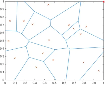
Figure 3.2: A figure of a random uniform sensor deployment with 16 sensors with Voronoi parti-tions created in Matlab. The red cross is the sole point of W which attains the cost as distance to the closest sensor and belongs toW3.
2
Non optimality of the grid
Figure 3.3: A sensor deployment with a lower cost than the grid deployment forp= 1. The red crosses are the points in the Voronoi regions which are the farthest away from the closest sensor. Since only 5 crosses can be seen, there must be some overlap.
In figure 3.3 a sensor deployment with a lower cost than a grid deployment can be seen. The cost of the grid and the improved deployment with 9 sensors, p= 1 are 0.2357 and 0.2341. However the difference between the costs is very small, it is shown that the performance of the grid is not optimal withp= 1. When the probability on active sensors decreases the grid is performing relatively worse. For the uniform deployment less is known about the cost. The sensors are drawn from a uniform distribution over [0,1]×[0,1] and therefore the expected location of the sensor is in the middle. The expectation of the cost however is not as simple as that and depends on the location of other sensors, as well on the probability p on active sensors. Though it may be the case that the random uniform deployment is better than the grid deployment for smallp.
3
Simulation results
Now some simulation results will be described and examined. The simulations are done as de-scribed in chapter 2 and the cost is estimated by an average of the costs of all simulation runs. The cost in a simulation run is the maximal distance from each of the distances from any points in W1, W2 and W3 to the closest sensor. Each run the grid deployment is constructed and a
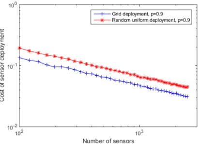
In figure 3.4 the estimated costs of the random uniform and the grid deployment with a probability on active sensors equal top= 0.9 are shown with logarithmic scales. As expected the grid performs better than the random uniform deployment for largep. In the plot with the logarithmic scales can be seen that the estimated costs of the grid deployment and random uniform deployment seem to approximate two straight lines which are parallel to each other. Therefore, a logarithmic relation between the number of sensors and the cost of both the deployments can be expected. From figure 3.4 it is also expected that the asymptotic cost (n→ ∞) is not equal for the grid and random uniform deployment withp= 0.9
Figure 3.4: This graph shows the estimated costs of the grid deployment (p= 0.9) and the random uniform deployment (p= 0.9) for square numbers of sensors. Both the axis are logarithmic.
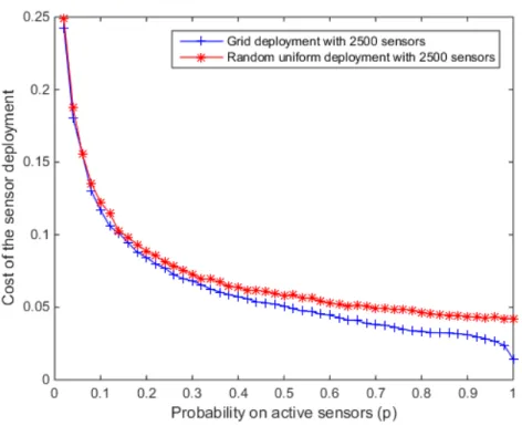
In figure 3.5 can be seen how the cost behaves when the probability on active sensors increases from 0 to 1 in 50 steps. With p ≈ 0 the difference between the cost of the two strategies is small and the cost is decreasing when p increases. So the grid always seems to have similar or better results regardless of the value ofp. Therefore, it can be concluded that the grid is a better strategy than the random uniform deployment. However, as already stated in this report, the grid deployment is not the optimal deployment, even forpequal to 1.
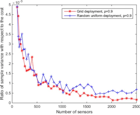
In both the simulations each setting with a different probability on active sensorspor a different number of sensors n is repeated 100 times. Then an average is taken over all these repetitions, but then it is important to know whether 100 repetitions is enough or whether the variance is rather high. Therefore the variance of the simulations is discussed here. Because the probability distribution of the cost is unknown, the sample variance (s2 = 1
n−1
Pn
i=1(yi−y¯)2) will be used
Figure 3.5: The costs of the grid and random uniform sensor deployments for different valuesp.
Whenp is fixed and the number of sensors increases a similar result can be seen in figure (3.7) where the ratio is decreasing as the number of sensors is increasing. This can be explained by looking at a grid deployment. The grid deployment shows much symmetry and thereby the cost is often attained at more than one point and by more than one sensor. This means that there are various different active sets of sensors with the same cost and thus the sensor deployment is less affected by the sleeping sensors which can be at different locations. When the number of sensors increases, the number of different active sets sensors with the same cost increases, therefore the variance is relatively smaller for larger number of sensors.
Chapter 4
Cost analysis
In this chapter the cost and behavior of the cost is examined. First a general lower bound for the cost will be constructed and Theorems from other researches are stated which are relevant to the cost of the sensor network within this research. However, they need to be adapted and interpreted in the right way as they do not explicitly state a relation between the cost, the number of sensors and the probability on active sensors. Furthermore, with use of the theorems a new theorem will be stated and then the results of all the theorems will be compared to the simulations done with the grid and random uniform sensor network.
1
A general lower bound
In this section a new lower bound will be constructed. With this new lower bound a minimal cost can be calculated for arbitrary numbers of sensors and each value ofp. The lower bound that will be constructed will be based on dividing the unit square surface into different squares. Then the will be looked at what happens when one of the squares does not contain any active sensors. This will result in a theorem about a lower bound for the cost for any sensor deployment. Formally the lower bound is described as follows.
Theorem 4.1 (General lower bound). Let n sensors be deployed on the square unit surface and letpbe the probability on an active sensor, then for each sensor deploymentx, and every∈(0,1), the cost of the sensor networkC(x)satisfies, for sufficiently largen
C(x)≥(1−)0√.8
2
s
−log (np)
nlog (1−p). (4.1)
Proof. Divide the square unit surface into squares with sides√2α2qlog (np)
πpn , then the length from
the middle of the square to a corner is equal to the half of the diagonal, that is: α
q
log(np) npπ .
Then, the surface is divided into k= 2α2πpnlog (np) (rounding errors are neglected) of such squares
containingn1,n2,..,nk sensors each. Now the cost is at least the length from the corner of a square
to the middle of the square if there is at least one square which contains no active sensors. If such a square can be found with a probability of at leastq, then we get that
C(x)≥qα
s
log (np)
Now, such a q > 0 will be specified. The probability of a square j having no active sensors is ¯
pnj = (1−p)nj. Because the probability on active sensors is independent, the probability on all
squares having some active sensors is equal to
Q= (1−p¯n1)(1−p¯n2). . .(1−p¯nk)≤e−pn¯ 1e−pn¯ 2. . . e−pn¯ k. (4.3)
This must be bound above by 1−q. Now turning it into the logarithmic of Q and using an inequality of arithmetic and geometric means one obtains
−logQ≥
k
X
j=1
¯
pnj ≥k
k Y j=1 ¯
pnj
1/k
=k(¯p)n/k. (4.4)
Using the value ofk above, this results in
−logQ≥ πnp(¯p)
n2α2 log (πpnnp)
2α2log(np) =
π(np)2α2 log (1πp −p)+1
2α2log(np) . (4.5)
Name the right side of equation (4.5)c∗. Nowαcan be chosen, such that the exponent of npis
positive, thenc∗ is always positive andc∗→ ∞ ifn→ ∞:
α2< −πp
2 log (1−p). (4.6)
Then −logQ→ ∞ forn→ ∞ and for eachn,−logQ > 0. This means that Qis smaller than 1, and it can be bounded from above by 1−q. Since −logQ ≥ c∗ is equal to Q ≤ e−c∗ and
1−q≥Q, it follows thatq≤1−e−c∗. Now chooseq= 1−e−c∗ to attain the largestqto make
the lower bound as large as possible. Then from equation (4.2) a lower bound is attained. Now
for sufficient largen, choosingα= 0.8q2 log (1−(πp)−p) results in a largec∗ such thatq= 1−e−c∗≈1.
Usingq∈(0,1) the cost of a sensor networkxcan be bounded by below by
C(x)≥qα
s
log (np)
npπ =q
0.8
√
2
s
−(πp) log (1−p)
s
log (np)
npπ =q
0.8
√
2
s
−log (np)
nlog (1−p). (4.7) Becauseq∈(0,1), it can be written as 1−, where∈(0,1) to indicate that it is close to 1 and to obtain (4.1).
With this theorem a lower bound for the cost for general sensor networks is defined with the only assumption that nmust be large enough. In the theorem a constant in αis chosen as 0.8. The choice of this constant affects the lower bound as it changes the value of q and α. The optimal constant can be found by maximizingqαsubjected toα2< −πp
2 log (1−p)and a closed form expression
can be found containing the Lambert function. However this optimal solution does not add much improvement and therefore the derivation is not shown in this report.
2
Known theorems about sensor coverage
stated in an article about coverage in mostly sleeping sensor networks[6]. This paper is about finding necessary conditions which imply coverage for a sensor network with high probability for inactivity and the number of sensors going to infinity. In this paper important theorems are stated on the coverage conditions of the grid and random uniform deployments.
Now the theorems for the coverage conditions of the grid deployment will be given, however first some assumptions which are required to state the theorems. Throughout the paper it is assumed that an eventT(x) almost always occurs if limx→∞P r[T(x)] = 1. Also, the radius r, probability
on active sensors pand defined parameter c are functions of the number of sensorsn. Assumed is that lim supn→∞p < 1, np → ∞ as n → ∞ and r → 0 as n → ∞. Besides that φ(np) is a slowly growing function which monotonically increases and goes to infinity as n → ∞ and
φ(np) =o(log lognp). Lastly the parameterc is defined as
c(n) = npπr
2
log (np). (4.8)
Now two theorems on coverage condition for the grid are stated, the proof can be found in the paper.
Theorem 4.2 (Grid coverage condition). If, for some slowly growing functionsφ(np), p, and r
satisfy
c(n)≥1 + φ(np)(1 +
p
plog (np)) + log log (np)
log (np) (4.9)
for sufficiently largen, then the entire unit square region is almost always covered.
Theorem 4.3(Grid non-coverage condition). Assumelimn→∞p= 0. If, for some slowly growing function φ(np),pandrsatisfy
c(n) = 1−φ(np)(1 + p
plog (np)) + log log (np)
log (np) (4.10)
for sufficiently largen, then the entire unit square region is almost always not covered.
For the random uniform deployment, similar conditions hold.
Theorem 4.4 (Random uniform coverage condition). Let n sensors be deployed uniformly over a unit square region. If, for some slowly growing functionφ(np),pandr satisfy
c(n)≥1 +φ(np) + log log (np)
log (np) (4.11)
for sufficiently largen, then the entire unit square region is almost always covered.
Theorem 4.5 (Random uniform non-coverage condition). Let n sensors be deployed uniformly over a unit square region, and assume limn→∞pr2 = 0. If, for some slowly growing function
φ(np),pandrsatisfy
c(n) = 1−φ(np) + log log (np)
log (np) (4.12)
So these 4 theorems are coverage conditions for the grid and random uniform deployment. This means that if these conditions hold, the square unit surface is almost always (not) covered and an explicit relation for the radius, the number of sensors and the probability on active sensors can be stated. However, the known theorems state coverage conditions instead of relations between the cost and the number of sensors and the probability on active sensors. Therefore they must be rewritten such that they can be compared with the simulations and the derived lower bound. This is done by using the value ofc=log (np)npπr2 whereris considered the sensing radius of a sensor
xand equations (4.9), (4.10), (4.11) and (4.12) can be rewritten as:
r≥ s
log (np) +φ(np)(1 +pplog (np)) + log log (np)
npπ (grid, coverage) (4.13a)
r=
s
log (np)−φ(np)(1 +pplog (np))−log log (np)
npπ (grid, no coverage) (4.13b)
r≥ s
log (np) +φ(np) + log log (np)
npπ (random uniform, coverage) (4.13c)
r=
s
log (np)−φ(np)−log log (np)
npπ (random uniform, no coverage) (4.13d)
These equations describe the conditions for the cost of a sensor deployment for which the unit square surface is almost always (not) covered under the assumptions listed in this section. There-fore, it is expected that the cost of a grid sensor deployment is larger thanrin equation (4.13b), but lesser or equal thanrin equation (4.13a). For the random uniform deployment the costC(x) is expected to be in between the values of r in equations (4.13d) and (4.13c). Now using the probability that the whole square unit surface is covered, a new theorem can be derived about the sensor cost.
Theorem 4.6. Let n sensors be deployed uniformly over a unit square region, then under the assumptions of theorem 4.5 a lower bound for the costs can be stated as
C(x)≥r−−o(r−) asn→ ∞, (4.14)
where r− = qlog (np)−φ(np)−log log (np)
npπ as in equation (4.13d) (where the unit square surface is
almost always not covered).
Proof. LetJ(x) be the cost of a random sensor deployment with a random set active sensorsA. Then the probability that the area Q is covered by the sensor deployment xwith the active set sensors A is equal to: Pr(Q is covered) = Pr(J(x)≤ r). Now the cost of a sensor deployment
C(x) is the expectation ofJ(x) and is equal to
C(x) =E(J(x)) =
Z
√
2
0
1−Pr(J(x)≤r)dr=
Z
√
2
0
Pr(J(x)> r)dr. (4.15)
Now the known theorems can be used to split up the integral. Letr−be therfrom the condition that the random uniform deployment is not covered (equation (4.13d)) and r+ the r from the condition that the random uniform deployment is covered (equation (4.13c)). Now the integral can be split up in 3 terms
Z
√
2
0
Pr(J(x)> r)dr=
Z r−
0
Pr(J(x)> r)dr+
Z r+
r−
Pr(J(x)> r)dr+
Z
√
2
r+
Pr(J(x)> r)dr (4.16)
LetE+ and E− be the events that the unit square surface is covered or is not covered. Then if
covered ifn→ ∞, i.e. limn→∞Pr(E+) = 1. Thus the minimal sensing radius, such that the area
is covered, r =r+ should still result in limn→∞Pr(E+) = 1. So the sensing radius required to
cover the square unit surface is almost always smaller than r+: limn→∞Pr(J(x)≤r+) = 1, so
limn→∞Pr(J(x)> r+) = 0. A similar argument can be used to a sensor network with a sensing
radiusr=r− almost always does not cover the unit surface, i.e. limn→∞Pr(E−) = 1. So with a
sensing radius smaller than or equal to r− the unit surface is almost always not covered, so the cost of sensor deployment is almost always larger thanr−: lim
n→∞Pr(J(x)≥r−) = 1. Now these
results can be used to obtain a lower bound for the cost of a random uniform deployment which holds for large numbers of sensors. The discussion above implies that Pr(J(x)> r+) = 0 +o(1)
and Pr(J(x)≥r−) = 1−o(1). Using this result, one can obtain
C(x) =
Z r−
0
1−o(1)dr+
Z r+
r−
Pr(J(x)> r)dr+
Z
√
2
r+
0 +o(1)dr
C(x) =r−(1−o(1)) + (√2−r+)o(1) +
Z r+
r−
Pr(J(x)> r)dr C(x)≥r−(1−o(1)) =r−−o(r−).
(4.17)
So from the theorems stated in [6], a lower bound for the cost is derived which holds for large n
and random uniform deployments. For the grid deployment, an assumption is made thatp→0 as
n→ ∞, therefore similar statements cannot be made due to the assumptions of the theorems. For the random uniform deployment the assumption is made thatpr2→0 asn→ ∞, this is the case
in this research as the cost of a sensor deploymentC(x)→0 asn→ ∞and can be interpreted as
r→0 asn→ ∞. In the simulations this lower bound will be simulated asr− as it should give a good estimation and it is not known how largeo(r−) is.
3
Comparison with simulations
In this section the results from the known theorems from the paper will be compared with the derived general lower bound and the simulation data from chapter 3 of the random uniform de-ployment and the grid dede-ployment. To do this, simulations of both the grid dede-ployment and the random uniform deployment will be made and the costs of these simulations will be compared with the lower and upper bounds derived from the theorems, described by equation (4.13). Doing this, the performance and correctness of the theorems will be tested and more information will be provided. The theorems from the paper contain a variableφ(np) which is a slowly growing function of the ordero(log log (np)), which needs to be specified in order to do simulations. This function is used for the proof of the theorem and considered whenn→ ∞. Therefore we can choose it as a small constant multiplied byplog log (np), so the limit stays the same and the relation should hold. This way,φ(np) is very small and the required radius for coverage in equations (4.13a) and (4.13c) are almost equal. Besides that, the radius which should result in no coverage in equations (4.13b) and (4.13d) are larger and almost equal as well. Since the constant can be chosen that small that it approximates 0, this will be used in the simulations in order to obtain only 1 lower and 1 upper bound from the paper.
are stated for n → ∞ and so the asymptotic costs of both the deployments may be the same, or the random uniform can be even smaller. However, from the simulations this seems unlikely because in figure 3.4 the lines seem to be parallel.
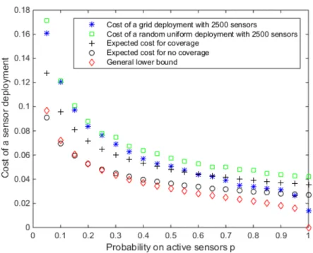
In the figures 4.1 and 4.2 the simulations of the cost of the random uniform and grid deployment, the expected lower and upper bounds from the paper and the general lower bound can be seen. As concluded in chapter 3 the cost of the random uniform deployment is larger than the cost of the grid deployment. The black pluses and circles are values of the radius at which the unit square surface is almost always covered and not covered. So it is expected that the cost of both the random uniform and the grid deployment are always in between these two values. For the grid deployment this is the case for largep, however the random uniform deployment always has costs above these values. Therefore it can be concluded that the theorems from the paper cannot be used in this research as an upper bound for the cost. The reason for this is probably the number of sensors, which is going to infinity for the theorem stated in the paper and thus may not be large enough in the simulations as the error seems to get smaller when the number of sensors increases. The lowerbound derived from the paper does seem to hold, except for the probability of active sensorspclose to 1 for the grid deployment. This may be caused by the assumptions on the grid deployment thatp→0 asn→ ∞, and as can be seen it does always hold for the random uniform deployment.
Figure 4.1: The simulated cost of the grid deployment and the random uniform deployment, the relations for the radius which implies coverage (4.13a) or no coverage (4.13c) and the general lower bound. The number of sensors n is varying from 102 to502 and the probability on active
sensors is kept equal atp= 0.9.
Chapter 5
Sensors deployment algorithms
In this chapter a deployment strategy is described made by an algorithm which aims to minimize the cost of a sensor deployment. This algorithm uses the gradient to compute a descent direction in which the sensors will move. The algorithm is much alike the algorithm designed in [3], but now also takes failure rates into account. This algorithm will be described and analyzed on convergence. Then a second algorithm will be made which is derived from the first. This algorithm has quicker convergence in general, but will not be analyzed on convergence properties because it is much alike the first algorithm.
1
Gradient descent algorithm
The gradient descent algorithm starts with a random sensor deployment. Then at each iteration the cost is computed and the sensors will move in a direction which decreases the cost. In fact, the sensor at which the cost is attained in an set active sensors, will move towards the farthest point in its Voronoi partition. However, for each deployment there are many different possible sets active sensors and all of these will be taken into account. So the direction is based on a weighted sum of all farthest points in the Voronoi partitions for all possible sets active sensors. The set active sensors which is more likely to occur, will contribute more to the directions as it also does contribute more to the cost of the sensor deployment.
Now will follow the exact algorithm description. As stated, the algorithm is a gradient descent algorithm where at each iteration the location of the sensor changes based on the gradient of the cost function. The objective function, (2.3) has to be minimized with respect to the sensor locations. So again the average cost of a sensor network must be minimized:
C(x) =X
A6=∅
P r(EA) max i∈A maxs∈Vi
ks−xik2. (5.1)
The algorithm is discrete and updates the sensor locations at each iteration. At each iterationkthe sensors locationsxk
i,i={1,2,..n}, will be updated tox k+1
i through the following equation:
xk+1=xk−α∇C(xk). (5.2)
In this formula,αis a positive constant smaller than 1 which should ensure convergence and the
s∈W. And letx∗A be closest active sensor to the points∗A. Assume that only 1 point be inW
and that the sensorx∗Ais unique. Then the cost function can be formulated as
C(x) =X
A6=∅
P r(EA)ks∗A−x
∗
Ak2. (5.3)
Then the gradient can be expressed as follows:
∇C(x) =∇x
X
A6=∅
P r(EA)ks∗A−x
∗
Ak2
=X
A6=∅
P r(EA)∇xks∗A−x
∗
Ak2.
(5.4)
The distance is defined as the euclidean distance, as a consequence the derivative of the norm is as follows:
Oxks−xk2=
x−s
ks−xk2
. (5.5)
This equation describes the direction from the pointsto the location of the sensorx, now by the minus sign from equation (5.2) it follows that the sensor will move in the direction of point s. From figure 5.1 it can be seen that for each active set of sensors, only 1 sensor will be move in the direction of the point at which the cost is attained. However, the direction in which a sensor will move is a weighted average over all the directions of all sets active sensors.
Figure 5.1: In this figure a sensor deployment with 9 active sensors can be seen together with the Voronoi diagram. The black plus is the only sensor that gains a direction with this active set of sensors, namely towards the red asterisk.
However, it is not necessary that the cost is attained at only 1 point by 1 sensor, therefore x∗
A
ands∗A do not have to be unique for all sets active sensors. To deal with the non uniqueness, the generalized gradient will be used which is defined as
∂f(x) =co{lim
In this equationcostands for the convex hull, Ωf is the set at whichf is not differentiable andS
denotes all sets with measure 0. In words the generalized gradient can be described as all possible convex combinations of all the possible derivatives which arise from the fact that the cost function
C(xk) has more derivatives when the cost is attained at more than 1 point or at more than one sensor. Now the generalized gradient can used in the update function. Letg(xk)∈∂C(xk), then the update function can be rewritten as:
xk+1=xk−αg(xk) (5.7)
Now instead of having one derivative which determines the direction the sensors will move to, all convex combinations of all possible derivatives can be used as a direction in which the sensor will move. This way the behavior of the solution of the algorithm does not have to be unique, this can be solved by taking the least-norm element ofg(xk)∈∂C(xk). The properties of the gradient
algorithm depend on the properties of the cost function C(x), therefore it will be checked if the cost functionC(xk) is locally Lipschitz.
Definition 5.1. A functionf : RN →
R is locally Lipschitz near x∈ RN if there exist positive
constants Lxand such that|f(y)−f(z)| ≤Lxky−zkfor ally,z∈RN in the neighborhood ofx
such that kx−yk ≤and kx−zk ≤.
Proposition 5.1. C(x)is a locally Lipschitz for allx∈Q.
Proof. Letyi ∈Q, i= 1,2,...,nbe the locations of the sensors and let i be a 1×n vector with
small values such thatzi=yi+i, zi∈Q. Now anLxwill be specified and the functionC(x) will
be proven locally Lipschitz.
C(z)−C(y) = X
A6=∅
P r(EA) max i∈Amaxs∈Vi
ks−zik2−
X
A6=∅
P r(EA) max i∈A maxs∈Vi
ks−yik2
= X
A6=∅
P r(EA)(max i∈A maxs∈Vi
ks−yi−ik2−max i∈A maxs∈Vi
ks−yik2)
. (5.8)
Note that the Voronoi partitions within the summation are not the same because the Voronoi partitions depend on the locations of the sensors. Though a small changei in the location cannot
result in a cost difference of more than maxi∈Akik2 for each set active sensors. Now will be
explained why. Without loss of generality letA be the set active sensors and letC(zA)≥C(yA).
Now assume the cost C(yA) of the set active sensor is attained at a points. Then this pointsis
either a vertex of the Voronoi partition (s∈W1), or a point on the boundary ofQ(s∈W2∪W3).
Now if s is a point on the boundary of Q, the cost for this set active sensors can be increased at most maxi∈Akik2 if the closest active sensor moves a distance maxi∈Akik2 in the opposite
direction of s. So for this case, C(zA)−C(yA) ≤ maxi∈Akik2. If s is a vertex of a Voronoi
partition, then at least 3 sensors have the same distance to s. Therefore, moving only 1 of these sensors results in a different point with the largest distance to the corresponding sensor since the boundaries of the Voronoi partitions will be different. Therefore the maximal increase in distance is obtained if all the sensors with the pointsin its Voronoi partition move in the opposite direction ofs. Then the distance is again increase with at most maxi∈Akik2, so also for this case,
C(zA)−C(yA)≤maxi∈Akik2. Using this result, one can obtain:
C(z)−C(y) ≤ X
A6=∅
P r(EA) max i∈A kik2
≤max
Now it is known that the cost function is locally Lipschitz with Lipschitz constant equal to 1, the critical points can be defined as in [3].
Proposition 5.2. Since C(x) is a locally Lipschitz function, if it attains a local minimum or maximum atx, then0∈∂C(x), such axis called a critical point.
In the special case that the probability on active sensors is equal top= 1, the critical points can be described as circumcenters of the Voronoi partitions. This means that the sensor locations are in the middle of their Voronoi partition. With a grid deployment, this is always the case. So the sensor locations of a grid deployment are critical points at which a local minimum is attained. This minimum is a local minimum and not a global minimum as shown in chapter 2. Now will be looked at the regularity of the cost functionC(x).
Definition 5.2. A function f : RN →
R is regular at x∈ RN if for all v ∈ RN, the right
di-rectional derivative off: f0(x,v), exists and equals generalized directional derivative off: f◦(x,v).
Here the right directional derivative and the generalized directional derivative of f at x in the direction ofv∈RN are defined as:
f0(x,v) = lim
t→0+
f(x+tv)−f(x)
t f◦(x,v) = lim sup
t→0+,y→x
f(y+tv)−f(y)
t .
(5.10)
It follows that locally Lipschitz functions which are convex or concave are also regular, as a result
f(x) =kx−sk2 is regular for fixeds, since it is convex and locally Lipschitz. Now with help of
the following proposition from [8] it can be proved that the cost function is regular.
Proposition 5.3. Let {fk :RN →R|k ∈ {1,2,3,...,m}}be a finite collection of locally Lipschitz
functions near x∈RN. Consider f(x0) = max{fk(x0)|k∈ {1,2,3,...,m}}. Then, if I(x0) denotes
the set of indexesk for whichfk(x0) =f(x0), and if eachfi is regular at xfori∈I(x), thenf is
regular at x.
Now it can be shown that the cost functionC(x) is regular for all x∈Q, a property that will be used to prove convergence.
Proposition 5.4. The cost function C(x)from equation (5.1) is regular for allx∈Q.
Proof. With the help of the geometrical properties of the cost function as stated in chapter 2, the maximal distance from a sensorxi ∈Qto the closest pointsin its Voronoi partition can rewritten.
Therefore letWi
1,W2i andW3i be the points ofW1,W2andW3 which correspond to the sensori.
max
s∈Vi
ks−xik2= max
(
max
s∈Wi
1
ks−xik2,max s∈Wi
2
ks−xik2,max s∈Wi
3
ks−xik2
)
(5.11)
Then for each sensor, the maximal distance to the furthest point in the Voronoi partition is given as a maximum of a fixed finite set of locally Lipschitz and regular functions and therefore is regular by Proposition (5.3). Then the costC(xA) of a set active sensors can be written as:
C(xA) = max i
max (
max
s∈Wi
1
ks−xik2,max s∈Wi
2
ks−xik2,max s∈Wi
3
ks−xik2
)
. (5.12)
which is equal to the cost function C(x) is a sum of regular functions and thereby also regular. So the cost function is regular for allx∈Q.
Now the critical points are defined and some properties are derived, the convergence to the critical points must be examined. It is known that the negative gradient −∂f(x) is always a descent direction if 0∈/ ∂f(x). Therefore La Salle’s theorem will be used to prove convergence from the initial locations x0 to the critical points. However, before LaSalle’s theorem can be used some
more properties are required. Because the gradient is not continuous and can have more values if different sensors attain the cost in a set active sensors, the solutions to differential equation concerning the sensor locations, ˙x=f(x(t)), must be understood in the Filippov sense. A Filippov solution of ˙x=f(x(t)) on an interval [t0,t1]⊂Ris defined as an absolute continuous solution of
the differential inclusion
˙
x∈K[f](x),
where K[f](x) = \
δ>0
\
µ(S)=0
co{f(BN(x,δ)\S)}. (5.13)
In this formula, µ denotes the Lebesgue measure. Now the Lie derivative of a function can be defined, this definition will be used to prove convergence. For a locally Lipschitz function
g:RN →
R, the set-valued Lie derivative ofg with respect tof atxis defined as
Lfg(x) ={a∈R|∃v∈K[f](x) such thatζ·v=a,∀ζ∈∂g(x)}. (5.14)
Note that for eachx, the Lie derivative equals a closed and bounded, possible empty interval. The following theorem is a nonsmooth version of LaSalle’s invariance principle [9].
Theorem 5.1 (LaSalle’s invariance principle). Let g be a locally Lipschitz and regular function. Then for x0 ∈ R, let g−1(≤ g(x0),x0) be the connected component of {x ∈ RN|g(x) ≤ g(x0)}
containingx0. Then assume that the set g−1(≤g(x0),x0) is bounded and either maxLfg(x)≤0
or Lfg(x) = ∅ for all x ∈ g−1(≤ g(x0),x0). Then g−1(≤ g(x0),x0) is strongly invariant for
˙
x=f(x(t)). Let Zf,g =
x∈RN |0∈Lfg(x) , then any solutionx starting at x0 converges to
the largest weakly invariant setM contained in Z¯f,g∩g−1(≤g(x0),x0).
With use of this theorem it can be proved that the sensors locations converge to the critical points. Instead of the discretized system, the continuous system will be used to prove the convergence. From the results from the continuous system we can conclude that with proper choice of the constant α the discrete system has the same convergence properties. Let the cost function be defined asC(x) from equation (5.1) and the movement of the sensorsxbe determined by
˙
x(t) =−∂C(x(t)). (5.15)
ThenQis a bounded area in which the sensorsxare, with initial sensor locationsx0. Now because
the area to which the sensors belong is bounded and the cost is always larger than zero and lesser than√2, the values of the cost functionC(x) are always bounded and so are the trajectories of the sensorsC−1(≤C(x
0),x0).
Theorem 5.2. Let x0∈Qbe the locations of the sensor and letC−1(≤C(x0),x0)be the bounded
trajectories of the sensors. Then any solutionx: [t0,∞)→RN of (5.15) starting atx0 converges
asymptotically to the set of critical points ofC(x)contained in C−1(≤C(x0),x0).
Proof. Let a ∈ L−∂C(x(t))C(x), then by the definition of the Lie derivative, there exists a w ∈
K[−∂C](x) =∂C(x) such that a=ζ·wfor all ζ∈∂C(x). Now the particular choice ζ=−w∈
∂C(x) givesa = −kwk2 ≤ 0. Therefore, maxL
−∂C(x(t))C(x) ≤ 0 or L−∂C(x(t))C(x) = ∅. It is
asymptotically to the largest weakly invariant set M contained in ¯Zf,g∩C−1(≤C(x0),x0). This
in fact are critical points where 0∈∂C(x).
So now it is proven that the continuous system converges for all possible initial locations to the set of critical points. From there we can deduce, that if the continuous system is discretized as in (5.7), the sensors locations converge to the set of critical points when the scalar α is chosen properly.
Remark 5.1 (coincident sensors). In the simulations, but also in the continuous case it may happen that sensors fall together on the same location. At that point, the incident sensors have equal Voronoi Partitions and therefore will be merged. Then the direction of the merged sensor is the same as the two original sensors and the probability on being active must be adjusted to
1−(1−p)2. The event that two sensors have incident locations may have 2 reasons, namely the
scalarαmay be too large, or the sensors converge to the same location. The scalarαonly affects the discrete case where the sensors move in specific directions such that they fall exactly together. This is a bad choice ofαwhich must be avoided and shows that it should have been chosen smaller. For values ofpvery close to 0, the sensors will all move too the middle and they can converge to the same location: [0.5,0.5]. This is not a problem, but the sensors converge in this case to critical points. When two sensors converge to the same locations, the regularity of C(x) is not affected and the function remains locally Lipschitz.
Simulations are done in order to see the actual results of the gradient algorithm. For these simula-tions, the initial sensor locationsx0are drawn from a random uniform distribution over [0,1]×[0,1].
The cost is computed as described in chapter 2 by considering all points of W1,W2 andW3 and
compare which one has the largest distance to the closest sensor. The constant αinfluences the convergence of the algorithm, if it is chosen very small the algorithm will certainly converge, but it may take a lot of stepsk and thereby too much time. In these simulations α is chosen equal to 5001 which gives good results, but does not take too much time. Because at each stepk the cost for all possible sets active sensors is computed to assign new locations for the sensors at step k+ 1, the algorithm is rather slow and the number of sensors exponentially increases the computational time. Besides that only 1 sensor gains a new direction for each active set sensors and as a result the convergence is slow. Therefore, the number of sensors cannot be very large and is chosen asn= 9 as the cost of the deployment can be can be compared to a grid deployment.
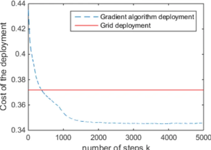
In chapter 2 it is already shown that the grid deployment is not optimal forp= 1 and the algorithm can make a deployment strategy with lower cost. Then the constructed deployment has Voronoi partitions which seem more alike hexagons instead of the squares from the grid deployment. In figure 5.2 can be seen what happens when the algorithm is applied to an initial sensor deployment
x0with 9 sensors andp= 0.9. The cost seems to be converging to a local minimum and the grid
Figure 5.2: A simulation outcome from the gradient descent algorithm with 9 sensors. At the left side the initial sensor locationsx0, in the middle the paths of the sensors throughout all 5000 steps
and at the right the final sensor locations.
2
Gradient based algorithm
In this section an algorithm will be described which is very similar to the gradient algorithm, but should have faster convergence. Because the aim to minimize the cost is the same as with the gradient algorithm, the objective function C(xk) remains the same and is as in equation (5.3).
Also the update step is similar to (5.7), but now the gradient will not be used. In this algorithm, each set active sensors will contribute to the directions in which all sensors in the set will move. This means that not only the sensor which attains the cost will gain direction, but also the other sensors will. Let h(xk) be the direction in which the sensors will move, than update function is
defined as:
xk+1=xk+αh(xk). (5.16)
Hereαis a constant which should ensure convergence. The directionh(xk
i) of a sensoriis chosen
as the weighted average over all directions towards the farthest points in the Voronoi partitionsVi
of all possible sets of active sensors in whichiis contained. Now it may happen that more points in the Voronoi partition attain the maximal distance to the sensor, in that case a convex combination is allowed as direction. Now the direction of a sensori, h(xki) can be written as:
h(xki)∈H(xki) =
X
A6=∅,i∈A
P r(EA)co{s−xik|ks−xkik2≥ kt−xkik2,∀t∈Vi, s∈Vi},∀i∈[n]
(5.17) In the figures 5.4 and 5.5 a simulation with this gradient based algorithm can be seen. The result of this algorithm is very similar to the results shown in 5.2 and 5.3, however the convergence is a bit faster. The faster convergence is due to the fact that at each step active set of sensors the sensors are moving towards the circumcenter of their Voronoi partition, which is in general the best way to lower the cost. In general the simulation has much quicker convergence, especially when the sensors start clustered in a corner. Besides for p= 1, the algorithm works much faster as it does move all the sensors, while the gradient descent algorithm only moves 1 sensor at each step.
Figure 5.4: A simulation of a sensor deployment with 9 sensors made with the algorithm based on the gradient descent algorithm. At the left side the initial sensor locations x0, in the middle the
Figure 5.5: The cost of the deployment at the stepskin the algorithm together with the cost of the grid deployment.
Because the algorithm is very similar to the gradient algorithm, the critical points and the conver-gence is not analyzed. The set of critical points is not exactly the same set, but is closely related. To make a good comparison between the two algorithms, simulations have been done for 5 differ-ent initial sensor locations (9 sensors), sampled according to the random uniform deploymdiffer-ent. In figure 5.6 on the next page the costs for the two algorithms can be seen for 5 different initial sensor locations. As can be seen, 4 out of 5 times the gradient based algorithm is decreasing faster than the gradient algorithm, which suggests that the non gradient algorithm has faster convergence in most cases. For the gradient algorithm 5000 update steps is not always enough for convergence and the cost still seems to be decreasing for some initial conditions. For the non gradient algo-rithm, the cost seems to be stabilized below the cost of the grid deployment for all different initial conditions.
Besides that it can be seen that the gradient algorithm always has a decreasing cost, while the gradient based algorithm has small drawbacks. This brings up the question whether the directions
Chapter 6
Discussion
In this chapter the results of this research are discussed. The theorems and performance of the gradient and non gradient algorithm will be discussed here. This will be done starting at the first chapter and then working down to the last chapter about the algorithms.
First of all the cost function which expresses the quality of a sensor network by looking at the average cost. This because the number of failures is probabilistic and therefore not known, so an average should give a good estimation of the expected cost. However, the cost of an active set of sensors is chosen as the worst case measurement which may not be as logical. The maximal distance from any point to the closest sensor may be an extreme way to measure the quality and instead the quality could be expressed as an integral over the whole domain of a function depending on the distance of each point to the closest sensor. This might result in a more stable network but as can be read in [2] it causes the sensor to tend to be more in the middle and the points near the boundary are less important. However the choice for the cost as a the maximal distance to the clos-est sensor in some cases corresponds to the disk-covering problem of which much more is known [1].
In chapter 2 the grid and the random uniform deployment strategies are discussed. Both these strategies are natural but suboptimal heuristic deployment strategies. In the one-dimensional case the performance of the equispaced sensor network was optimal for the case that sensors may not fail. Therefore it was expected that the grid would perform optimal as well without failures. From the simulations with the gradient it is known that the grid is not optimal. This itself is a good result, however the optimal solution still cannot be described explicitly by any deployment, even without failures. However the structure of the optimal solution without failures seem to have a hexagon Voronoi structure. In [3] an algorithm is defined to find the locations of the sensors which give local minimal cost. In that research it is proven that the problem is equal to finding sensor locations which are the circumcenters of their own Voronoi partition. Thereby, it can be concluded that the optimal solution is a deployment where the sensor locations are circumcentres of their Voronoi partition, however there will remain more possible solutions to this problem and an optimal solution cannot be described.
to cover the whole area, than for the grid deployment as can be seen in (4.13a) and (4.13c). This arises the expectation that the radius or cost of the uniform deployment should be smaller than that of the grid deployment. This is in none of the simulations the case, however the failure rate is assumed very small in the theorem and the number of sensors is very large. This might be the reason for the lower requirement and it might be the case that for low chances on active sensors, the asymptotic cost of the random uniform grid is lower. Besides that the general lower bound which is constructed in this paper, still yields some assumptions and thereby may not hold for small number of sensors and small probabilities on active sensors. This is also a bit dissatisfying, because if the theorems will be implemented, it is probably not very common that a very large number of sensors are deployed.
Chapter 7
Conclusion
In this research the cost of sensor deployments are analyzed on several things. Firstly the cost a sensor as defined in this research has only 3 sorts of points which determine the actual cost of an active set of sensors. The cost is defined by the worst measurable point in the area, because of that the problem of finding the lowest cost with no failing sensors is very similar to the disk-covering problems. However, this measure of the cost of a sensor deployment did not allow a linear program such as in the one-dimensional case in which the optimal cost and sensor placement could be com-puted. To analyze the behavior of the cost when more sensors are used or different probabilities on active sensors, a grid deployment and a random uniform deployment were introduced. From the one-dimensional case it was expected that the grid is optimal with no inactive sensors, it can be shown that this is not the case in the two-dimensional setting. Also, from the simulations it is expected that the both the deployments have a cost which depend logarithmic on the number of sensors.
Instead of finding the optimal cost, creating lower and upper bounds for the cost will also provide information about the cost behavior. Therefore theorems of a paper which state coverage condi-tions were rewritten to a relation about the radius. From these condicondi-tions a lower bound is made for the random uniform deployment for large numbers of sensors, but due to the assumptions, no other lower or upper bounds could be made. Besides that, a more general lower bound was constructed for the cost which also holds for a large enough number of sensors. This general lower bound is under most circumstances less strict but can be used in more settings.
Chapter 8
Recommendations
In this chapter, recommendations will be done for further research. Due to the time limit some things are not done in this research, besides that, choices were made which influences the research and with different choices, different results can be obtained.
The first thing on which more research can be done is a different cost function. In this research, the cost function is defined as a weighted average over all possible sets active sensors and then the cost for an active set sensors is the farthest distance from a point to the closest sensor. Instead of looking at the worst measurable point, one can look at all points and take the average over the whole field. This can be done by replacing the maximal value by an integral over the whole area. Then the boundary of the area on which the sensors are placed may have a smaller influence, especially for small number of sensors.
Instead of changing the cost function, the area itself could be changed as well. In some researches the area is already varied as a polygon and as long as the area is convex, the model should still be applicable with some minor adjustments. Though it can help arise more understanding for the optimal cost and the cost behavior for different probabilities on active sensors.
Probably the most interesting is finding and optimal solution for the problem of robust sensor coverage. As a start of finding the optimal solution, an optimal solution can be searched for in the case that the probability on active sensors is equal to 1. In this research it is already shown that the grid deployment is not optimal, but instead a honeycomb alike structure seems to have better results and may even be optimal. Then the task is to find how the honeycomb should be defined and how it changes, when the area which must be covered changes. Then if an optimal deployment is found with no failing sensors, it may be used to derive a general solution for when failing sensors are allowed. Besides that it may be of use to make a better and more general lower bound for the cost of the sensor network.
Bibliography
[1] F. Bullo, J. Cort´es, and S. Martinez, Distributed Control of Robotic Networks. Princeton University Press, 2009.
[2] S. Hutchinson and T. Bretl, “Robust optimal deployment of mobile sensor networks,” pp. 671– 676, 2012.
[3] J. Cort´es and F. Bullo, “Coordination and geometric optimization via distributed dynamical systems,”SIAM Journal on Control and Optimization, vol. 44, no. 5, pp. 1543–1574, 2005.
[4] J. Cortes, S. Martinez, T. Karatas, and F. Bullo, “Coverage control for mobile sensing net-works,” in Robotics and Automation, 2002. Proceedings. ICRA’02. IEEE International Con-ference on, vol. 2, pp. 1327–1332, IEEE, 2002.
[5] S. Shakkottai, R. Srikant, and N. B. Shroff, “Unreliable sensor grids: Coverage, connectivity and diameter,”Ad Hoc Networks, vol. 3, no. 6, pp. 702–716, 2005.
[6] S. Kumar, T. H. Lai, and J. Balogh, “On k-coverage in a mostly sleeping sensor network,” pp. 144–158, 2004.
[7] P. Frasca, F. Garin, B. Gerencser, and J. M. Hendrickx, “One-dimensional coverage by unre-liable sensors,” arXiv preprint arXiv:1404.7711, 2014.
[8] F. H. Clarke,Optimization and nonsmooth analysis. Siam, 1990.