Explicit calculations of automorphic forms for definite unitary groups

University of Warwick institutional repository: http://go.warwick.ac.uk/wrap

This paper is made available online in accordance with

publisher policies. Please scroll down to view the document

itself. Please refer to the repository record for this item and our

policy information available from the repository home page for

further information.

To see the final version of this paper please visit the publisher’s website.

Access to the published version may require a subscription.

Author(s): David Loeffler

Article Title: Explicit Calculations of Automorphic Forms for Definite

Unitary Groups

Year of publication: 2008

Link to published article:

http://dx.doi.org/10.1112/S1461157000000620

EXPLICIT CALCULATIONS OF AUTOMORPHIC FORMS FOR

DEFINITE UNITARY GROUPS

DAVID LOEFFLER

Abstract

I give an algorithm for computing the full space of automor-phic forms for definite unitary groups over Q, and apply this

to calculate the automorphic forms of levelG(ˆZ) and various

small weights for an example of a rank 3 unitary group. This leads to some examples of various types of endoscopic lifting from automorphic forms for U1×U1×U1 and U1×U2, and to an example of a non-endoscopic form of weight (3,3) corre-sponding to a family of 3-dimensional irreducible`-adic Galois representations. I also compute the 2-adic slopes of some au-tomorphic forms with level structure at 2, giving evidence for the local constancy of the slopes.

Contents

1 Introduction 2

2 Outline of the algorithm 2

2.1 Definitions . . . 2

2.2 Hecke operators andK-classes . . . 3

2.3 A refinement . . . 5

3 Example: E=Q( √ −7) 6 4 Experimental results: level 1 7 4.1 Dimensions of spaces . . . 7

4.2 Forms arising from Gr¨ossencharacters . . . 8

4.3 Forms arising from classical modular forms . . . 8

4.4 Interpretation: Satake parameters . . . 9

4.5 Galois representations . . . 9

4.6 Matching weights . . . 10

4.7 A non-endoscopic form . . . 10

5 Some higher level examples 11 5.1 L-classes . . . 11

5.2 The operatorU . . . 13

5.3 Automorphic forms and slopes . . . 13

Received 22 January 2008, revised 11 August 2008;published???. 2000 Mathematics Subject Classification 11F55

c

6 Implementation details 14

6.1 Algorithms forr-good matrices . . . 14 6.2 Programs included with this paper . . . 15

7 Acknowledgements 15

1. Introduction

IfGis a reductive algebraic group overQ, then the spaces of automorphic forms

for G (of a given level and infinity-type) are well-known to be finite-dimensional vector spaces with an action of the Hecke algebra. However, for the vast majority of groups it is not known how to actually calculate the dimensions of these spaces and how the Hecke operators act. For GL2, the case of classical modular forms, there are well-known algorithms based on modular symbols (see e.g. [12]), but in general little is known.

One case in which calculations are possible is where the group G satisfies the condition that all arithmetic subgroups are finite. In this case, Gross has shown [7] that the theory of automorphic forms can be set up entirely algebraically, without analytic hypotheses. As has been observed by various authors [8, 4], Gross’s spaces are (at least in theory) computable. In this article, I shall apply this to an example of a definite unitary group over _Q, and show how the full space of automorphic forms may be calculated for various small weights and levels. We do not need to assume that the class number ofGis 1; we do assume that the underlying quadratic extension of_Qhas class number 1, but this is more a calculational convenience than a fudamental limitation of the algorithm.

The results of these computations give rise to some interesting specimens of endoscopic liftings of automorphic forms arising fromU2×U1 and U1×U1×U1,

and also examples of non-endoscopic forms, which give nontrivial families of 3-dimensional`-adic Galois representations.

The structure of this paper is as follows. Section 2 explains the algorithms used to determine the class number of G and the coset decomposition of the Hecke operators; these depend on the choice of level groupKbut not the weight. In section 4, we use the results of these computations to calculate the spaces of forms of various small weights. In section 5, we shall see how to generalise this to non-maximal level groups, and present some examples illustrating the 2-adic continuity of the Hecke eigenvalues. In the final section, we discuss some implementation details.

2. Outline of the algorithm

2.1. Definitions

Recall that if E is an imaginary quadratic number field andn _> 1, there is a corresponding definite unitary groupG=Un,E, which is the group scheme over Z

defined by

G(A) ={g∈GLn(A⊗_ZOE)|gg† = 1},

Proposition 2.1. G(R) is the usual real unitary group Un, which is connected

and compact. Ifp is any prime which splits completely inE, then G is split at p, and moreoverG(_Qp)is isomorphic toGLn(Qp). There are two such isomorphisms,

corresponding to the two embeddings E ,→ _Qp, and they are interchanged by the

inverse transpose involution of GLn. The centre of G is the norm torus U(1) = Res(1)_E/

Q(Gm).

SinceGis compact at infinity, it certainly satisfies the conditions of [7]; so the space of automorphic forms forGof levelK(whereKis an open compact subgroup of G(_Af)) and weight V (whereV is an irreducible algebraic representation of G over any fieldFof characteristic 0) is theF-vector space of functionsf :G(_Af)→V such that

f(γgk) =γ◦f(g) ∀γ∈G(Q), k∈K.

For the rest of this paper, we shall fixn= 3; however, the methods can clearly be applied to arbitraryn, and indeed to general totally definite Hermitian spaces over OE(of any integral equivalence class). We shall, however, make the simplifying as-sumption thatEhas class number 1. Initially, we shall takeK=G(ˆZ) =Q`G(Z`), so we obtain the automorphic forms of “level 1” in some sense.

Remark 2.2. Ifpis not ramified in E, the subgroupK is a hyperspecial maximal compact subgroup of G(Qp). If pis ramified, then K is special maximal but not

hyperspecial, unlessp= 2 in which case it is not even maximal [11, §1.10].

Theorem 2.3. The irreducible algebraic representations ofGoverE (or any field

containing it) are parametrised by triples of integers (a, b, c) with a, b _> 0, where the representation Va,b,c is the unique highest weight direct summand of Wa,b,c = SymaV ⊗SymbV∗_⊗detc _{(where V =V}

1,0,0 is the standard representation). The central character ofVa,b,c is



 z

z z



7→za−b+3c.

Proof. SinceGis isomorphic toGL3 overE, this follows from standard results on the representation theory ofGL3, see e.g. [5,§15.5].

Remark 2.4. We can identify Va,b,c explicitly: there is a natural contraction map

Wa,b,c → Wa−1,b−1,c, and Va,b,c is the kernel of this map. We shall not use this remark, however, as in the calculations below we will always have already calculated automorphic forms of weight (a−1, b−1, c) when we come to deal with those of weight (a, b, c); thus we can easily identify forms which we have seen before.

2.2. Hecke operators and K-classes

It is well known that the set of double cosets

G(Q)\G(Af)/K

is finite. We shall refer to these asK-classes. As shown in [7], ifµ1, . . . , µris a set of representatives for theK-classes, then the space of automorphic forms for Gof levelK and weightV is isomorphic to

r

M

where Γi = G(Q)∩µiKµ−i 1, via the map f 7→(f(µ1), . . . , f(µr)). Note that the groups Γg are arithmetic subgroups ofG, and are thus finite.

If we know a set of class representativesµi and the associated groups Γi, then it is elementary to calculate the Γi-invariants in Va,b,c for eachi and thus read off the dimension of the space of automorphic forms.

The other piece of information we are interested in is the action of the Hecke algebra. This is the commutative algebra generated by double cosetsKgK, with the action of such a coset on automorphic forms being given by

([KgK]f) (x) =X j

f(xgj)

whereKgK=F_g

jK.

So we must decomposeKgK into single cosetsgjK. For each of these, we could choose a coset representative in the form γjµc(j), for some c(j) ∈ {1. . . r} and γj ∈G(Q). This would immediately allow us to calculate ([KgK]f) (1), iff is an

automorphic form given as anr-tuplef(µ1), . . . f(µr), since

([KgK]f) (1) =X j

f(γjµc(j)) = X

j

γj◦f(µc(j)).

What we actually want, however, is ([KgK]f) (µi); so for eachi∈ {1, . . . , r}we need to find elementsγij∈G(Q) andc(i, j)∈ {1, . . . , r}such that

µiKgK =

G

j

γijµc(i,j)K.

For any given elementg∈G, finding these quantities is a finite search. In fact, one has:

Algorithm A. Let r,s,t be given elements ofG(Af), which are integral outside a finite setS of primes split in E. Then the following algorithm finds all elements ofG(Q)∩rKsKt:

1. Find some λ∈ OE such that λrst, regarded as an element of GL3(Af,E), is

integral at all places ofE.

2. Enumerate all matricesg∈M3(OE)such that gg† = Norm(λ).

3. For eachgin the above list, setγ=λ−1_{gand calculate the elementary factors} ofr−1_γt−1 _{at each prime inS. If these coincide with those ofs, outputγ.}

Calculating the elementary factors of a p-adic matrix is easy, but in practice one can often short-cut this step, since ifνpλis small then there are very few pos-sibilities for the elementary factors and these can be distinguished by calculating the determinant. The most computationally intensive step is usually (2). For con-venience, let us define an r-good matrix to be an element of M3(OE) such that

gg† =r. Enumerating all ther-good matrices for a givenris clearly a finite check, but possibly a long one ifris large – an algorithm using lattices is described in§6.1 below.

double cosetsKηK, whereη is one of the elements

ηp,1= 



1 1

p/p



, ηp,2= 



1 p/p

p/p



, ηp,3= 



p/p p/p

p/p



.

These are the operators to which we shall apply the above method. We shall writeTp,ifor the operator on automorphic forms corresponding to the double coset

Kηp,iK. Note thatTp,3 is central, and acts on weight (a, b, c) forms as scalar

mul-tiplication by (p/p)a−b+3c. 2.3. A refinement

The above discussion assumes that the class representativesµiare known. How-ever, we can use a sort of bootstrapping approach to find the class representatives at the same time as the Hecke operators.

Lemma2.5. The double cosets Kηp,1K andKηp,2K both containp2+p+ 1single

cosets.

Proof. This is a purely local computation. We shall consider η = ηp,1; the other

case is very similar. LetH =G(_Zp); thenHacts transitively by right multiplication on row vectors over_Fp, andH∩ηHη−1is the stabilizer of the line (0,0,∗). So this subgroup has index |_P2₍

Fp)| =p2+p+ 1; and thus HηH should decompose into

p2_{+p+ 1 single cosets (which can easily be written down explicitly).}

Now, let us assume that we know a set of representatives for a subset of the class set; we can always start with just the principal class G(Q)K, represented by the

element 1. Let us choose a primep. Using Algorithm A above, we can find all of the single cosets contained inKηp,1K which have a representative of the formγµ withγ∈G(Q) andµone of the subset of class representatives we know about.

If we have found less thanp2+p+ 1 cosets, then the lemma shows that we have not found the full class set, and moreover, taking a local coset representative gives an explicit elementµofG(Af) (supported atp) which is not in any of theK-classes previously found; so we can add this to the list, calculate the associated group Γ (by applying Algorithm A again, withs= 1) and repeat.

Clearly, we need a criterion which will allow us to determine when we have found the complete class set. To do this, we shall introduce the mass of K, which is a quantity strongly related to the class number but in many ways better behaved; this can be calculated via the special value of an appropriateL-function.

Definition2.6. The mass of a compact open subgroupK of G(Af), whereGis a

connected reductive algebraic group compact at∞, is the quantity

Mass(K) = X

[g]∈G(Q)\G(Af)/K 1 #Γg.

A mass formula for unitary groups is given in [6]. This applies to a somewhat more general class of unitary groups than we consider here, so we shall state a special case: if G is the unitary group Un,E as defined above and n is odd, and

K=G(ˆ_Z), then

Mass(K) = 1

2n ·L(M)·τ(G)·

Y

p

HereL(M) is the value ats= 0 of theL-function of the motive ofG;τ(G) is the Tamagawa number ofG; and the local factorsλp are 1 unlesspis ramified inE, in which case they are 1₂. (Forneven, there is a similar formula but the local factors are all 1.)

Formulae forτ(G) andL(M) are known, and are given in [6]. For unitary groups we haveτ(G) = 2; and ifχis the Dirichlet character corresponding to the quadratic extensionE/Q, then

L(M) = n

Y

r=1

L(1−r, χr).

which is easy to compute using generalised Bernoulli numbers as in chapter 4 of [14].

Remark 2.7. Knowing the mass in advance allows one to determine whether the full class set has been found; but it is not completely clear that this will ever actually occur – that is, that every K-class occurs in the decomposition of some Hecke operator. On the other hand, one can show (using the assumption thatEhas unique factorisation and strong approximation for the derived subgroupSU3,E, cf [10, ch. 7]) that every K-class does have a representative supported atpfor every prime p. Hence if computing Tp,1 and Tp,2 for enough p does not find enoughK

-classes, one can switch to computing multiple Hecke operators at some fixed small prime. However, I am not aware of any case in which this is necessary.

3. Example: E=_Q(√−7)

To illustrate the algorithm above, we shall carry out the calculations in the case

E=Q(

√

−7). This choice is convenient, as thenGis split at 2, and O×_E =±1, so

G(Q)∩K is small (it is the group of monomial matrices with entries inO×E, and thus has order 48). Letω= 1+

√ −7

2 , soOE=Z[ω].

We shall begin by calculating the mass of K. Here χ is the Kronecker symbol −7

•

; using standard methods we find that L(0, χ) = 1, L(−1, χ2_{) = −}1 12 and L(−2, χ3_{) =−}16

7, so L(M) = 4

21. Hence

Mass(K) =1 8 ·

4 21·2·

1 2 =

1 42.

Since ₄₂1 > ₄₈1, the mass of the principalK-class, there must be otherK-classes; we shall find them by the bootstrapping argument explained above.

If p is any split prime and p a choice of factor of pin E, then we can apply Algorithm A to find the setG(Q)∩Kηp,1K, takingλ=p. For instance, let us take

p= 2 and choosepto be the ideal generated byω. Then we find 288 such matrices; sinceG(Q)∩K has order 48, this gives us 6 right cosetsγK, which are represented

by the three diagonal matrices with entries 1,1,_1−ωω in some order, and the three permutations of the rows of





1 0 0

0 ω₂ −ω

2

0 ω₂ ω₂



.

primesp6= 2 and under the isomorphismG(_Q2)∼=GL3(Q2) corresponds to 



1 0 0

0 1 0

−1 −1 2



.

The associated group Γα has order 336; indeed it is isomorphic to the direct product of±1 with a simple subgroup isomorphic toP SL2(F7). Conveniently, this

group contains G(_Z) as a subgroup of index 7; it is generated by G(_Z) and the element

τ =





−1 2

1−ω

2 1 2

−1 2

−1+ω

2 1 2

ω

2 0

ω

2 

.

of order 7.

Since ₄₈1 +₃₃₆1 = ₄₂1 = Mass(K), that’s all: the class number ofGis 2.

We can now complete the calculation of the Hecke operatorTp,1 as follows. In

the notation of the previous section, we are takingµ1 = 1 and µ2 =α. We have

decomposedµ1KηK as a union of 6 cosets of the form γµ1K and 1 coset γµ2K.

Searching for rational elements ofµ2KηK (using Algorithm A with λ= (1−ω)2)

finds 7 cosets already, so we do not need to consider the fourth possibility, which is whether there are any elements ofG(Q)∩µ2KηKµ−21.

Since we have now found the complete class set, it is clear how to calculateTp,i for any split prime p. Note that we need to apply Algorithm A four times, with

λ=p,ωp,ωpand 2p, so we need to enumerater-good matrices forr=p, 2pand 4p.

Remark 3.1. Calculating Hecke operators at the inert primes is also possible, but more awkward both theoretically and computationally. Since the maximal split torus inG(_Qp) forpinert has rank 1, there is only one Hecke operator to deal with, but calculating its coset decomposition requires enumerating r-good matrices for

r=p2_{, which rapidly becomes computationally infeasible. Also, the eigenvalues of}

these Hecke operators are rather more indirectly related to Galois representations.

4. Experimental results: level 1

In this chapter I’ll summarise the calculations I have made for various small weights. Note that there are no forms of weight (a, b, c) ifa+b+cis odd since the level group contains−1; and changingc by a multiple of 2 just induces a twist, so I shall restrict to the case wherec= 0 ifa+bis even andc= 1 ifa+bis odd; this is what is meant by “weight (a, b)”.

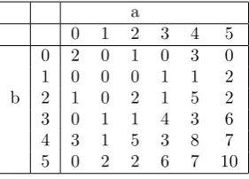
4.1. Dimensions of spaces

These can be deduced from classical results of invariant theory for actions of groups on polynomial algebras. See table 4.1.

a

0 1 2 3 4 5

0 2 0 1 0 3 0

1 0 0 0 1 1 2

b 2 1 0 2 1 5 2

3 0 1 1 4 3 6

4 3 1 5 3 8 7

5 0 2 2 6 7 10

Table 1: Dimension of spaces of automorphic forms

4.2. Forms arising from Gr¨ossencharacters

For small weights, many of the forms that arise appear to haveTp,1 eigenvalues

of the form χ1(p) +χ2(p) +χ3(p), where χi(p) = prps for some (r, s). Note that there exists an unramified Gr¨ossencharacter ofEsending a uniformiser atptoprps whenever r+s is even, as E has unique factorisation and unit group ±1; let us writeχ(r, s) for this character.

In all cases other than the constant function, we find that the characters arising haver+s= 2. In table 4.2 below I list these, based on calculating Hecke operators at all split primesp₆60. (I have assigned arbitrary numbers to Gal(E/E)-orbits of eigenforms, in order of discovery.)

Weight Form Character

(0,0) 1 χ(0,0) +χ(1,1) +χ(2,2) (0,0) 2 χ(2,0) +χ(1,1) +χ(0,2) (2,0) 1 χ(4,−2) +χ(1,1) +χ(0,2) (4,0) 3 χ(6,−4) +χ(1,1) +χ(0,2) (2,2) 2 χ(4,−2) +χ(1,1) +χ(−2,4)

Table 2: Forms arising from Gr¨ossencharacters

4.3. Forms arising from classical modular forms

Other forms of small weight appeared to haveTp,1eigenvalues given byχ(r1, s1)+ χ(r2, s2)ap for ap the Hecke eigenvalue attached to a classical modular newform. Note that this class includes all of the forms above (some in multiple ways), since for eachrthere exists a CM-type modular form of weightr−1 withap=χ(r,−r)+

χ(−r, r). The automorphic forms on U(3) that are associated with non-CM-type forms are listed in Table 4.3 below.

Weight Form Character Modular weight Modular label

(4,0) 1 χ(1,1) +χ(0,−4)ap 7 7k7B[3]1

(4,0) 2 χ(0,2) +χ(1,−4)bp 6 49k6E1

(3,1) 1 χ(1,1) +χ(−1,−3)ap 7 7k7B[3]1 (2,2) 1 χ(1,1) +χ(−2,−2)ap 7 7k7B[3]1 (3,3) 1 χ(1,1) +χ(−3,−3)cp 9 7k9B[3]1

In the third column of the table, I have reused letters when the same modular form occurs more than once. The labels in the final column are those used in William Stein’s online tables.

Note that aboveχ(r, s) was defined only for r+seven. If r+sis odd, there is no unramified Gr¨ossencharacter sending a uniformiser at p to pr_ps

– indeed, this is not well-defined as the choice of generator of the ideal p is only defined up to ±1 – but there is a unique Gr¨ossencharacter which is unramified outsideλ=√−7, whose restriction toO(Eλ) is the order 2 character ofF×7, and whose restriction to E∞=Cisz7→z−rz−s; this character sends a uniformiser atp to pλ

pr_ps , which is independent of the choice of generator ofp. This is what is meant byχ(1,−4) in the above table.

4.4. Interpretation: Satake parameters

Recall that the Satake parameters of an unramified representationπpofGL3(Qp)

are the eigenvalues of the semisimple conjugacy class that is the Langlands param-eter of the representation πp. These can be obtained as the roots of the Satake polynomial

X3−tp,1X2+ptp,2X−p3tp,3

wheretp,iis the eigenvalue ofTp,ion theGL3(Zp)-invariants ofπp. It is conjectured that ifπp is the local factor of a cuspidal automorphic representation, then (with the normalisations we have chosen) the Satake parameters are algebraic numbers whose complex absolute values are all equal top.

The automorphic forms we have encountered are all (vacuously) cuspidal except the constant form. For the forms in Table 4.2 and Table 4.3 above, the Satake pa-rameters are easy to read off: for Table 4.2, the Satake papa-rameters are the values at p of the three characters listed, and for Table 4.3, the Satake parameters for

χ1+χ2ap are{χ1(p), χ2(p)α, χ2(p)β}whereαandβare the Satake parameters

as-sociated to the formf. The normalisation that is conventional for classical modular forms of weightkgives bothαandβ absolute valuep(k−1)/2_{. Thus the characters} χ(r, s) in Table 4.2 are forced to have r+s = 2; and for characters of the form

χ(r1, s1) +χ(r2, s2)ap, we’d better haver1+s1= 2 andr2+s2= 3−k.

4.5. Galois representations

Let f be an eigenform of weight (a, b, c) and level G(ˆZ). By results of Blasius

and Rogawski [1], for each prime `there is a semi-simple representation

ρf : Gal(E/E)→GL3(Q`)

unramified outside 7` and crystalline at `, such that for p= pp any other prime split inE not dividing 7`the characteristic polynomial of ρf(Frobp) should be the

Satake polynomial off atpas defined above.

(The proofs of this statement in the literature assume that the weight is “reg-ular”, i.e. a 6= 0 and b 6= 0. For non-regular weights, `-adic interpolation in the manner of [3, Ch. 1] gives a representation with values in GL3(<sub>C</sub>`) as long as `

splits in the field E, but it is not clear whether it is crystalline. It is, however, necessarily Hodge-Tate.)

Heretp,i is the eigenvalue ofTp,i onf, so in particulartp,1is the trace of

forms are correct, the associated representations ρf decompose as direct sums of smaller-dimensional representations (sums of three characters, or of a character and a twist of a 2-dimensional modular representation).

If ` is a prime split in E, then we can restrict the representation to a decom-position group at either of the primes above `. Since this local representation is crystalline, it is certainly Hodge-Tate; but the weights at these two different primes are not generally the same – for one decomposition group the weights will be −b+c, c+ 1, a+c+ 2 and for the other the weights will be−a−c,−c+ 1, b−c+ 2. This fits the tables above, asχ(a, b) has weightaat one prime andb at the other, and the representation associated to a modular form of weightkhas weights 0 and

k−1 (whichever prime is used).

4.6. Matching weights

Given a fixed weight (a, b, c)∈N×N×Z, the constraints of the valuations of

Satake parameters and the Hodge-Tate weights at the two primes above`leave few possibilities for endoscopic forms at this weight.

We shall supposec= 0; then it is clear that if aandb are both even, then the character χ(a+ 2,−a) +χ(1,1) +χ(−b, b+ 2) is the unique combination of χ’s which gives the appropriate Hodge-Tate weights and satisfies the Satake condition

r+s= 2. This explains why we have seen one eigenform of this type whena,bare both even and none otherwise.

The situation for automorphic inductions of modular eigenforms is more compli-cated. The representation associated to a classical modular eigenform of weight k

has Hodge-Tate weights 0 andk−1, and the Satake parameters atphave complex absolute valuesp(k−1)/2_{, so characters of the formχ(r1, s1) +χ(r2, s2)a}

p can only appear whenr1+s1= 1 andr2+s2+ (k−1) = 2. Checking all the possible cases, we find that there are potentially 3 families of automorphic eigenforms onU3, with weights andTp eigenvalues given by

χ(1,1) +χ(−s,3−k+s)ap weight (k−3−s, s,0)

χ(2−r, r) +χ(1,2−k)ap weight (k−2, r−2,0)

χ(r,2−r) +χ(2−k,1)ap weight (r−2, k−2,0)

4.7. A non-endoscopic form

Weight (3,3) is the first case where the action of the Hecke operators is not diagonalisable overE. One obtains two Hecke-invariant subspaces of dimension 2, corresponding to Galois orbits of eigenforms.

The first subspace splits over E(√46), and the Tp,1-eigenvalues are χ(1,1) + χ(−3,−3)cp, wherecp is the unique Galois orbit of modular eigenforms of weight 9 for Γ1(7) such that c2 is defined over this field. In this case,Tp,2 coincides with Tp,1.

The second space is more interesting. HereTp,1andTp,2commute with each other

and have the same eigenvalues, but are not identical; so for the two eigenforms in the orbit, theTp,1-eigenvalue of one form is theTp,2-eigenvalue of the other form

polynomial for one of the primes above 2 is

X3−−7 + √

−259

8 X

2₊−7−

√ −259

4 X−8.

Since the Satake polynomial is irreducible overE(√−259), the Satake parameters are all Gal(E/E)-conjugate; so none of them arise from Gr¨ossencharacters of E, and thus the corresponding `-adic Galois representations must be irreducible of dimension 3.

Let’s check the valuations of the Satake parameters. It can be shown [9] that a cubic over C has all its roots of equal valuation if and only if, after scaling so

the constant terms is 1, it is of the formT3_+aT2_{+aT+ 1 with alying inside a}

deltoid in the complex plane with centre 0 and one cusp at 3; this is equivalent to

a=x+iy with x, yreal such that

C(x, y) = (x2+y2)2−8x(x2−3y2) + 18(x2+y2)−27₆0.

In this case we find thatC(x, y) =−56727

4096, so the condition is satisfied.

5. Some higher level examples

We shall now introduce some level structure at the prime 2. In preparation for future work in which I intend to consider overconvergent automorphic forms, we shall use a slightly different definition of automorphic forms in which the action is twisted to the other side. We shall fix a prime p which is split in E and an irreducible algebraic representation V of G (which will be defined over Qp), and

consider functions

f :G(_Af)→V such that f(γgk) =k−p1f(g)

for allγ ∈G(Q) and k∈K for some open compact K. This is isomorphic to the

previous space, via the map f(g) 7→gp◦f(g) (if we fix a choice of embedding of

E ,→Qp), but has the advantage that we only ever need to consider the action on V of elements ofKp; this is useful when consideringp-adic interpolation, as in [3] or my University of London PhD thesis (in preparation).

The action of the Hecke algebra on this space is slightly different: we define an action of a double coset KgK on automorphic forms of level K by writing

KgK=F_g

iK, and defining

([KgK]◦f)(x) =X i

(gi)pf(xgi).

It’s easily verified that this gives a well-defined linear endomorphism of the space of automorphic forms.

5.1. L-classes

We shall setp= 2; and we will define our level groupLto beG(_Z`) at all`6= 2, and at 2 the subgroupLp ofGL3(Z2) which reduces mod 2 to





∗ ∗ ∗

0 ∗ ∗

0 ∗ ∗



This is the parahoric subgroup associated to a parabolic subgroup ofGL3. We now

need to calculateL-classes and decompositions of Hecke operators for this case.

Lemma 5.1. Let U0 ⊂ U be any finite index subgroups of G(Af). Then we have

Mass(U0) = [U :U0] Mass(U).

Proof. This is an essentially trivial but fiddly manipulation.

Mass(U0) = X

[v]∈G(Q)\G(Af)/U0

1 |G(Q)∩vU0v−1|

= X

[µ]∈G(Q)\G(Af)/U

X

k∈U/U0

1

|G(Q)∩µkU0k−1µ−1|·

1 size of orbit ofk

(where we consider the action ofU∩µ−1_G(

Q)µonU/U0 by left multiplication)

= X

[µ]∈G(Q)\G(Af)/U

X

k∈U/U0

1

|G(_Q)∩µkU0_k−1_µ−1_|·

|G(Q)∩µkU0k−1µ−1|

|G(_Q)∩µU µ−1_|

= Mass(U)·



 X

k∈U/U0

1





= Mass(U)·[U :U0]

It’s readily seen that Lp is the subgroup of matrices inGL3(Z2) whose

reduc-tion modpstabilises (∗,0,0)T _{under the left multiplication action on column} vec-tors; GL3(Z2) clearly acts transitively on these, so [K : L] =|P1(F2)|= 7. Hence

Mass(L) =₄₂7 = 1₆.

The proof of the above lemma indicates how to work out theL-classes, by cal-culating, for eachK-classG(Q)µK, howK∩µ−1G(Q)µacts by left multiplication

onK/L, which we can identify withP1(F2).

For the identityK-class, the groupG(Q)∩K consists of a product of diagonal

±1’s (which all reduce to the identity and can be ignored) and permutation matrices. So the action corresponds to permutation of coordinates on P1(F2), which has

exactly 3 orbits classified by the number of nonzero terms. Coset representatives

are given by: the identity (having stabiliser of order 16); the matrix





1 0 0

1 1 0

0 0 1





(again with 16); and the matrix





1 0 0

1 1 0

1 0 1



with stabiliser of order 48.

For the nonidentityK-class, the extra generatorτ ofG(Q)∩αKα−1conjugates

to an element ofG(Af) whose matrix reduces mod pto





1 1 1

1 0 1

1 0 0



This acts transitively on the elements of _P2₍

F2), so G(Q)αK = G(Q)αL. The

stabilizer group must thus have size 48, and it is easy to enumerate its elements as it is a subgroup of the finite group Γαof the previous two chapters.

5.2. The operator U

Motivated again by the theory of overconvergent automorphic forms, we consider the action of the Hecke operator corresponding to the double cosetLηp,2L, where pis the prime above 2 generated byω. As the role it plays is roughly analogous to the Atkin-LehnerUp-operator in Coleman’s theory, we shall denote it by the letter

U.

To decompose Lηp,2L into single cosets locally, we observe that if η = ηp,2,

then Lp∩ηLpη−1 consists of those elements of Lp whose first column reduces to (∗,0,0)T mod 4. This is an index 4 subgroup of Lp and coset representatives φi may be obtained by taking the first column to be (1,0,0)T, (1,2,0)T, (1,0,2)T and (1,2,2)T_{. We hence obtain a decomposition ofLηL as}F4

i=1φiηL.

As in the levelKcase, the final step is to write each single coset in terms of our chosenL-class representativesµ1. . . µ4, and more generally to do the same for the productsµrφsηL. This is easy using an adaptation of Algorithm A: we note that if

γ ∈G(Q) satisfies γµt ∈µrφsηL, then the largest denominator that can possibly occur inγ has norm either 2, 4 or 8, depending on (r, s, t). We then generate lists of the 2, 4 and 8-good matrices, and for each coset µrφsηL, we use these to find a representative for this coset in the formγµt(testing each of the possible values of t in turn until one works). Note that we must explicitly test φ−s1µ−r1γµ−

1

t for membership ofL, rather than dodging this check using elementary factors as before. The results of this computation are shown in Table 5.2.

Remark 5.2. Since the groupLp we have chosen is a parahoric subgroup, one can attach invariants to double cosets LpgLp ⊂ GL3(Qp) (analogous to elementary factors) using the Bruhat–Iwahori decomposition. One can probably use this to calculate the Hecke operators more efficiently; but the slower method above is more flexible and would apply to any groupL for which we could computeK/L

andL/(L∩ηLη−1_).

5.3. Automorphic forms and slopes

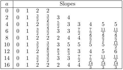
The coset representatives calculated in Table 5.2 above can now be used to calculate automorphic forms of level L using the same machinery as before. The choice of level structure and ofU operator should imply that the resulting objects interpolate well 2-adically as the acomponent of the weight varies. See Table 5.3 for a table of the 10 smallest 2-adic slopes of the U operator on forms of weight (a,0,0), for various integers a (necessarily even). This table shows clear evidence of the 2-adic local constancy of the slopes.

Note that the slopes ofU are not remotely locally constant with regard to vari-ation in theb direction in the weight lattice; indeed the dimension of its ordinary subspace grows asbgets large (in the archimedean sense!). This is unsurprising, as

µ1φ1ηL= 



1 0 0

0 1−w

2 0

0 0 1−w

2 

µ1L µ3φ1ηL=   w 2 − w 2 0 w 2 w 2 0

0 0 1



µ4L

µ1φ2ηL= 



1 0 0

0 1−w

2 0

0 0 1−w

2 

µ2L µ3φ2ηL=   w 2 w 2 0 −w 2 w 2 0

0 0 1



µ4L

µ1φ3ηL=





1 0 0

0 0 1−w

2

0 1−w

2 0



µ2L µ3φ3ηL= 



1 0 0

0 w₂ w₂ 0 w₂ −w

2  µ4L µ1φ4ηL=  

1 0 0

0 1−w

2 0

0 0 1−w

2 

µ3L µ3φ4ηL=   −w 2 w 2 0 w 2 w 2 0

0 0 1

 µ4L µ2φ1ηL=   w 2 − w 2 0 w 2 w 2 0

0 0 1−w

2 

µ1L µ4φ1ηL=   −w 2 − w 4 + 1 2 − w 4 + 1 2

0 −w

4 − 1 2 w 4 + 1 2 w 2 − w 4 + 1 2 − w 4 + 1 2  µ1L µ2φ2ηL=   w 2 w 2 0 −w 2 w 2 0

0 0 1−w

2 

µ1L µ4φ2ηL=   −w 4 + 1 2 − w 2 − w 4 + 1 2 w 4 + 1

2 0 −

w 4 − 1 2 −w 4 + 1 2 w 2 − w 4 + 1 2  µ1L µ2φ3ηL=  

0 w₂ −w

2

0 w₂ w₂ 1−w

2 0 0



µ2L µ4φ3ηL=   −w 2 − w 4 + 1 2 − w 4 + 1 2

0 −w

4 − 1 2 w 4 + 1 2 w 2 − w 4 + 1 2 − w 4 + 1 2  µ3L µ2φ4ηL=  

0 w₂ w₂

0 −w

2

w

2

1−w

2 0 0



µ2L µ4φ4ηL=   −w 4 + 1 2 − w 2 − w 4 + 1 2 −w 4 − 1 2 0 w 4 + 1 2 −w 4 + 1 2 w 2 − w 4 + 1 2  µ1L

Table 4: Decomposition of the double cosetLηL

and properties of these spaces. This space corresponds to allowingp-adic variation in theadirection but not thebdirection in the weight lattice.

A striking aspect of these tables of slopes is the fact that they are often non-integral. This is very much contrary to the case ofGL2where slopes are “usually” integral, at least for weights in the centre of weight space (Wan has conjectured that for any fixed weightkthe denominators of the slopes of overconvergent forms at weightkis bounded). Extending the computations above gave an example of a form with slope 74

7 at weight (5,5,0).

6. Implementation details

6.1. Algorithms forr-good matrices

The time-consuming step in Algorithm A, which was used in several places, is to calculate all elements ofGL3(OE) satisfying mm† =r; to calculate the Hecke operator at a split primepone needs to consider r=p, 2p, and 4p, so to have a reasonable supply of primes one needs to considerr≈100. Clearly this is equivalent to finding all orthogonal triples of vectors of length r in O3

6-a Slopes

0 0 1 2 2

2 0 1 3₂ 3₂ 3 4

4 0 1 2 5₂ 5₂ 3 3 4 5 5

6 0 1 3₂ 3₂ 3 3 7₂ 7₂ 11₂ 11₂

8 0 1 2 2 2 4 4 9₂ 9₂ 9₂

10 0 1 3₂ 3₂ 3 5 5 5 5 11₂

12 0 1 2 8₃ 8₃ 8₃ 3 4 5 6

14 0 1 3₂ 3₂ 3 3 7₂ 7₂ 11₂ 11₂ 16 0 1 2 2 2 4 4 14₃ 14₃ 14₃

Table 5: The 10 smallest slopes ofU acting on forms of levelLand weight (a,0,0), for evena₆16.

dimensional_Z-lattice. I experimented with two different algorithms, both of which have the same first step of generating a complete listL of the vectors of length r. This list is typically quite large – since the theta-function of the lattice O3

E is a modular form of weight 3 and level Γ1(7), it is easily seen that forr=p,2p,4pwith pa prime split inE, there are Θ(p2_{) such vectors (with leading terms that can be}

calculated precisely using Eisenstein series in each case).

The obvious algorithm is to regard this as a graph triangle enumeration prob-lem: consider the graph whose vertices are the vectors in L and where vertices

u, v are joined by an edge if they are orthogonal. This graph is typically not very dense, so from an appropriate sparse representation of its adjacency matrix one can enumerate all triangles in it quickly by a vertex-iterator approach. The most com-putationally difficult step is calculating the adjacency matrix: testing all possible pairs of elements ofLwill takeO(p4_{) steps.}

A more devious alternative is to calculate, for each vectorvof lengthr, a basis for the orthogonal complement ofvinO3

E, as a 4-dimensionalZ-lattice; enumerate vectors of length r in this; and find the orthogonal complement of these, to give orthogonal triples. This option turns out to be very much quicker for larger, as the orthogonal complement lattices typically have very few short vectors.

6.2. Programs included with this paper

Accompanying this paper is a selection of computer programs that were used in the calculations above; these can also be downloaded from my personal website at http://www.ma.ic.ac.uk/~dl505/maths/programs/programs.html. These use a combination of the Sage [13] and Magma [2] computer algebra systems; users who do not have access to Magma can still use the code for level 1 automorphic forms, but will be restricted to those primes for which precalculated lists ofr-good matrices are included.

7. Acknowledgements

support.

I am also grateful to Michael Stoll, for suggesting to me the second, more efficient lattice-based algorithm forr-good matrices described in§6.1 above.

References

1. _{Don Blasius}and _{Jonathan D. Rogawski}, ‘Tate classes and arithmetic quotients of the two-ball.’ ‘The zeta functions of Picard modular surfaces,’ (Univ. Montr´eal, 1992) pp. 421–444, pp. 421–444.

2. _{Wieb Bosma},_{John Cannon}and_{Catherine Playoust}, ‘The Magma al-gebra system. I. The user language.’ J. Symbolic Comput.24 (1997) 235–265.

3. _{Ga¨etan Chenevier}, ‘Famillesp-adiques de formes automorphes et applica-tions aux conjectures de Bloch–Kato.’ Ph.D. thesis, Universit´e Paris VII, (6 2003).

4. _{Lassina Demb´el´e}, ‘Quaternionic Manin symbols, Brandt matrices, and Hilbert modular forms.’ Math. Comp.76 (2007) 1039–1057 (electronic).

5. _{William Fulton} and _{Joe Harris}, Representation theory: a first course, vol. 129 ofGraduate Texts in Mathematics (Springer, 1991).

6. _{Wee Teck Gan}, _{Jonathan P. Hanke}and _{Jiu-Kang Yu}, ‘On an exact mass formula of Shimura.’ Duke Math. J. 107 (2001) 103–133.

7. _{Benedict H. Gross}, ‘Algebraic modular forms.’ Israel J. Math.113 (1999) 61–93.

8. _{Joshua Lansky} and _{David Pollack}, ‘Hecke algebras and automorphic forms.’ Compos. Math.130 (2002) 21–48.

9. _{David Loeffler}, ‘Adventures with polynomials: a criterion for Weil num-bers.’ Eureka 59 (to appear) Available from http://www.ma.ic.ac.uk/ ~dl505/maths/cubics.pdf.

10. _{Vladimir Platonov}and_{Andrei Rapinchuk},Algebraic groups and num-ber theory, vol. 139 ofPure and Applied Mathematics(Academic Press, 1994).

11. _{Jonathan D. Rogawski},Automorphic representations of unitary groups in three variables, vol. 123 of Annals of Mathematics Studies (Princeton Univ. Press, 1990).

12. _{William Stein}, Modular forms, a computational approach, vol. 79 of Grad-uate Studies in Mathematics (Amer. Math. Soc., 2007).

13. _{William Stein}, Sage Mathematics Software (Version 2.8.9). The Sage Group, (2007). http://www.sagemath.org/.

14. _{Lawrence C. Washington}, Introduction to cyclotomic fields, vol. 83 of

Graduate Texts in Mathematics (Springer, 1982).

David Loeffler [email protected]

Department of Mathematics Imperial College