Towards a Unifying Framework for Modelling and Executing Model Transformations

(1)

MASTER’S THESIS

Towards a Unifying Framework for

Modelling and Executing

Model Transformations

Ivo van Hurne

18

th

June, 2014

Supervisors: dr. L. Ferreira Pires

dr. C.M. Bockisch

(2)

(3)

A Thesis Submitted in Partial Fulfilment

of the Requirements for the Degree of

M

aster of

S

cience in

C

omputer

S

cience

at the

U

niversity of

T

wente

(4)

(5)

Abstract

Model-driven engineering is a software engineering technique which relies heavily on the use of models. They are not just used as documentation, but actually define the system. Transformations on the models are described using model transformation languages. There are a lot of different model transformation languages available, all having a different approach to model transformation.

We show that these languages are actually not that different at all. Based on the analysis of a varied selection of transformation languages we define a small number of primitive transformation operations that can be used to describe model transformations written in any transformation language. We define our own primitive transformation language, using just these operations, and verify our analysis by implementing a few well-known transformation languages in our own language, including a language not considered in the initial analysis.

We design an interpreter for our primitive language and show that the execution of model transformations with our interpreter is on par with their original interpreter.

(6)

(7)

Acknowledgements

I would like to thank a few people for their support during the writing of this thesis. First of all, I would like to thank Luís Ferreira Pires and Christoph Bockisch for taking over the supervision of the project. Without their help it probably would not have been possible to complete this thesis. I would also like to thank my fellow students at the SE-lab for their valuable feedback and support.

I’m indebted to Edwin Vlieg and Joost Diepenmaat for giving me the final push necessary to finish the project. Finally, I’m grateful to my family and friends for their never-ending support.

(8)

(9)

List of Figures

2.1. Kernel of Ecore model [1] . . . 6

2.3. Model transformation pattern (including metamodel) [2] . . . 8

3.1. Simple graph transformation example . . . 13

3.2. Henshin transformation units [3] . . . 18

5.2. Transformation engine architecture . . . 36

5.3. Thrascias Trace structure . . . 37

5.4. Thrascias abstract syntax . . . 38

6.1. Metamodels for mapping scenario [4] . . . 42

6.2. EMF ‘extlibrary’ metamodel (adapted from [5]) . . . 43

6.3. ‘extlibrary’ model after Pull Up Class Attribute transformation . . . 43

6.4. Model for refactoring scenario . . . 44

(14)

(15)

List of Tables

3.1. Language constructs in GROOVE control language . . . 15 3.2. A selection of Stratego language constructs . . . 19 3.3. Comparison of transformation operations at the rule level. . . 23 3.4. Comparison of transformation operations at the transformation level. . 24

4.1. Primitive transformation language operations . . . 29 4.2. Comparison of transformation primitives . . . 33

5.1. Thrascias operations . . . 39

(16)

(17)

List of Algorithms

3.1. Pseudo-code representation of single-pushout graph transformation. . . 14 3.2. Pseudo-code representation of Henshin’s execution algorithm. . . 17 3.3. Pseudo-code representation of the Stratego rule application algorithm. . 19 3.4. Pseudo-code representation of Stratego’s cascading transformation strategy. 20 3.5. Pseudo-code representation of the ATL transformation algorithm. . . . 22

(18)

(19)

1

Introduction

1.1. Motivation

TheModel-Driven Architecture(MDA) [6] was introduced in 2001 by the Object Manage-ment Group (OMG) to aid the integration, interoperability and evolution of software systems. MDA is an approach to specifying software systems that separates specifica-tion of funcspecifica-tionality from its implementaspecifica-tion on a specific technology platform.

Kent [7] introduced the term Model-Driven Engineering (MDE), which in a sense extends MDA. MDE is not only concerned with the separation of platform-independent from platform-specific, but also with the development process and extra dimensions like versioning. Contrary to MDA, MDE is not necessarily based on OMG standards. Instead it uses general standard-independent modelling concepts.

MDE relies heavily on the use of models. They are not just used as documentation but define the system at a high abstraction level, omitting any technology-specific information. A model can describe, for example, the structure or the behaviour of a system. The actual implementation of the system can be generated from such a model via a model transformation. Transformations can also be used for reverse engineering (implementation to model) and the transfer of information between systems.

In MDE, model transformations are usually defined using amodel transformation language. Research has led to the creation of several transformation languages and at present new languages continue to appear.

New model transformation languages can be useful to test and demonstrate novel ideas, and to specify languages tailored for a given domain. However, the development of these languages is a time-consuming process, as most of them are implemented from scratch and as such they are difficult to extend and adapt.

(20)

1.2. Objectives

Although the languages all have their own particular approach and features, they have the same main purpose. This means they are likely to share some common features. For example, in all transformation languages, models can be manipulated and navigated in some way (e.g. using OCL [8]). Languages often share common structures like transformation rules, and may provide control over the execution order of these rules. The objective of this work is to create a unifying framework for executing trans-formation languages that exploits the commonalities between a set of languages, while being able to execute of each one of them. This would enable faster prototyping of new ideas, easier reuse of (parts of) transformations and the composition of transformations written in different languages.

1.3. Research Questions

How can we execute different model transformation languages in a common envir-onment, while retaining the variability between the languages?

This question has been decomposed into three subquestions:

1. What should a common execution environment for model transformation lan-guages look like?

2. How do we build support for executing different transformation languages in this common environment?

3. What are the limitations of executing transformation languages in a common environment?

1.4. Research Approach

• We first take a look at the principles of models and model transformation lan-guages. Out of the vast amount of transformation languages available, we select a few representative languages for a more detailed analysis.

• Second, we investigate the execution algorithms of these languages. We look into the commonalities and variabilities, which results in a set of primitive transformation operations.

• Third, we define a language for specifying transformation languages in our common environment.

• Fourth, we implement an interpreter for our language in order to execute the specified languages.

(21)

1.5. Outline 3

1.5. Outline

(22)

(23)

2

Model Transformation Languages

We start with an introduction to model transformation and provide an overview of existing transformation languages.

2.1. Models

We mentioned before that models are the cornerstone of MDE. The wordmodelis used to describe lots of different concepts in different contexts. We will use the definition by Kurtev [9], which summarizes some of the existing definitions: “A model represents a part of the reality called the object system and is expressed in a modelling language. A model provides knowledge for a certain purpose that can be interpreted in terms of the object system.”

Most models conform to ametamodel, which is a model of a modelling language and basically describes its abstract syntax. Because a metamodel is itself a model, it is an instance of another metamodel (also known as ameta-metamodel).

2.2. Eclipse Modeling Framework

The Eclipse Modeling Framework (EMF) is a framework for modelling and code generation of applications based on structured data models [5]. In EMF, metamodels are defined as instances of the Ecore model. Additionally, the Ecore model itself is defined as an Ecore model.

Figure 2.1 shows the main part of the Ecore model [1]. EClasses are used to define classes along with their attributes (EAttribute) and references (EReference). EPackages can be used to group the classes.

(24)

[image:24.595.119.537.82.369.2]

ENamedElement EAnnotation EModelElement 0..n +eAnnotations 0..n +eModelElement ETypedElement EPackage 0..n +eSubpackages 0..n +eSuperPackage EParameter EClassifier 0..1 +eType 0..1 0..n +ePackage +eClassifiers 0..n EOperation 0..n +eOperation +eParameters 0..n EReference 0..1 +eOpposite 0..1 EDataType EAttribute +eAttributeType 11 EClass 0..n +eSuperTypes 0..n 0..n +eContainingClass +eOperations 0..n 0..n +eReferences 0..n 0..n +eAttributes 0..n EStructuralFeature +eContainingClass +eStructuralFeatures 0..n 0..n

Figure 2.1.: Kernel of Ecore model [1]

EMF provides basic Java code generation for its models, including a simple editor, support for basic model modification operations and persistence.

2.3. Model Transformation

In the Object Management Group’s MDA Guide, model transformation is defined as “the process of converting one model to another model of the same system” [6]. However, this definition does not include the specification of a transformation and unnecessarily restricts transformations to models of the same system. Additionally, it does not take into account transformation to and from multiple models.

(25)

[image:25.595.129.407.92.255.2]

2.4. Model Transformation Pattern 7

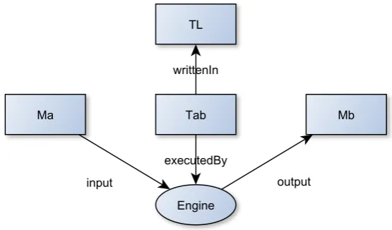
Figure 2.2.: Model Transformation Pattern

2.4. Model Transformation Pattern

Model transformations can be described using the pattern shown in Figure 2.2. We have a source model Ma, a target model Mband a transformation definitionTab. The

transformation definition is written in a transformation languageTL. When executed,

Tab transformsMa to Mb.

As mentioned before multiple source and target models can be used in the same transformation, extending the pattern accordingly.

As a model is an instance of a metamodel, we can extend the pattern to include the metamodels (Figure 2.3). Some transformation languages do not need metamodels because they operate on generic graphs or ASTs (e.g. GROOVE, Stratego). Other languages do need metamodels.

2.5. Transformation Languages

There are many different model transformation languages available, but they can never-theless be classified into a number of categories. Because we are mainly interested in the execution algorithms of model transformation languages, we consider four aspects for classification: transformation approach, rule application strategy, model representation

andtracing[11].

2.5.1. Transformation Approach

(26)

[image:26.595.193.461.96.313.2]

Figure 2.3.: Model transformation pattern (including metamodel) [2]

Declarative Approach The declarative approach is also known as the relational ap-proach. Developers specify relations between elements of the source and target models. The transformation language has to figure out the necessary transformation steps by itself. Examples of declarative languages are Henshin [3] and QVT Relations [12].

Imperative Approach The imperative approach is also known as the operational ap-proach. Developers specify the exact operations that have to be performed to transform source models to target models. An example of an imperative transformation language is QVT Operational Mappings [12].

Hybrid Approach A third approach has yet to be mentioned: the hybrid approach. Strictly speaking this is not an approach separate from declarative or imperative, but simply makes both available to the developer in a single language. An example of a hybrid language is ATL [13].

2.5.2. Rule Application Strategy

A transformation usually consists of a number of units. In most languages these units are rules [11]. Rules can appear in many guises, for example a rewrite rule with a left-hand side and a right-hand side; or a function that takes an input pattern and produces output by using an expression.

(27)

2.5. Transformation Languages 9

therefore use a strategy to choose the order in which transformation rules should be applied and at which model region. There are two kinds of strategies [11]:

Deterministic A deterministic strategy can either beexplicit orimplicit. In the first case the application order is defined by an explicit strategy, possibly separate from the transformation rules themselves (example: Stratego [14]).

In the second case the developer has but indirect control over the application order. The result of the transformation is deterministic, but can be changed by changing the matching patterns and logic of the rules (example: ATL [13]).

Non-deterministic In a non-deterministic strategy a rule and/or application location is chosen randomly from matching rules or model regions (example: graph transformation languages [15]). It is important to note that even if the application strategy is non-deterministic, the result of the transformation can still be non-deterministic, in case all the different application orders result in the same output model.

2.5.3. Model Representation

Models used by transformation languages can be represented in various ways. Some possibilities are graphs (e.g. graph transformation), abstract syntax trees (e.g. Stratego) and Eclipse Modelling Framework models [16] (e.g. Henshin, ATL).

2.5.4. Tracing

Traces record information about the execution of a transformation. Commonly traces are used to map source elements to target elements [11]. They can be used for analysing how changes in the source model affect the target models, for synchronizing models and for debugging.

There are various types of traces:

• Different kinds of information can be recorded, such as, the rule that created a trace or the time of creation.

• Information can be recorded at different abstraction levels, for example, only for top-level transformations.

• Information can be recorded for different scopes, for example, only for particular transformation rules.

• Traces can be stored in a number of locations, such as, in the source model, target model or in a separate location.

(28)

2.6. Languages to Consider

We choose to analyse five declarative model transformation languages. Based on the classification above, they have significantly different characteristics and they are well-known representatives of their kind.

Graph transformation Not really a language as such, but rather a class of transformation languages with graph-based models, a non-deterministic rule application strategy and no inherent tracing support.

GROOVE Graph transformation language extended with explicit deterministic rule application strategy. No inherent tracing support.

Henshin Eclipse modelling framework-based language with explicit deterministic rule application strategy. No inherent tracing support.

Stratego Abstract syntax tree-based term-rewriting language with explicit deterministic rule application strategy. No inherent tracing support.

ATL EMF-based language with implicit deterministic rule application strategy and inherent tracing support. Although ATL is a hybrid language we only consider its declarative part.

We discuss these languages in detail in Chapter 3. We choose only declarative languages, so we can validate our analysis later on using a language with a different transformation approach (imperative ATL).

2.7. Conclusions

(29)

3

Transformation Execution Algorithms

In Chapter 2 we have selected five transformation languages for further analysis: graph transformation, GROOVE, Henshin, Stratego and declarative ATL. In this chapter we take a look at the way they are executed and try to find commonalities between them.

3.1. Graph Transformation

The first execution algorithm we consider is the algorithm used in graph transformation. In this kind of transformation a model is described as a graph. There are multiple ways to do this, the most simple being the mapping of entities to nodes and relations to edges. However, once more complicated relations are used (e.g. multiplicity) more complicated mappings are necessary [17]. This, however, is outside the scope of this thesis.

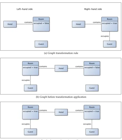
To transform a model, graph rules can be defined that specify pre-conditions for the application of a rule (calledleft-hand side) and post-conditions that have to be satisfied after the application of a rule (right-hand side) [15].

There are actually a number of different approaches to graph transformation that can be used. The way in which new elements are added and old elements are removed is slightly different for these approaches, but the general idea is the same. In this thesis we illustrate graph transformation using thesingle-pushout approach(SPO).

Algorithm 3.1 describes the approach in pseudo-code. We first select an arbitrary transformation rule. We try to find an arbitrary occurrence of its left-hand side L

(Figure 3.1a) in a graphG(Figure 3.1b). This happens in line 10 of Algorithm 3.1 using

G.getMatches(). During the matching that is taking place here, any possible negative

application conditions are also taken into account. Negative application conditions are conditions under which a rule should not be applied. For example, one could add

(30)

a condition to the rule in Figure 3.1a that prevents guests from occupying multiple rooms.

Once matches have been found, we iterate over them in a non-deterministic order. All graph elements that exist in Lbut not in Rare then deleted fromG (lines 12-14). Subsequently, we check for any dangling edges in G, and delete them (lines 16-19). Finally in lines 21-23, we add the objects that exist inRbut not in LtoG(Figure 3.1c) [18].

If a transformation rule has been applied successfully, the transformation is restarted and we again start to look for matches for an arbitrary transformation rule. If no matches were found for a transformation rule we try a different rule. The transformation ends when none of the transformation rules can be applied.

Because of the non-deterministic choice of rules there is no guaranteed confluence. This means executing the transformation multiple times on the same model does not necessarily yield the same result. Moreover, termination of a transformation is not guaranteed and a rule might not be executed even if there exists a match for this rule in the graph.

3.2. Controlled Graph Transformation

In a graph transformation, rules are self-contained units that specify the exact pre-conditions for their application [19]. Rule ordering is often a major reason for specifying these conditions. Because the conditions can be very complex and rules can implicitly depend on other rules, the transformation is not always easy to understand. A possible solution is to move the complex pre-conditions out of the rules, specifying them using so-called control expressions. In other words: an explicit deterministic rule application strategy is introduced.

3.2.1. GROOVE

Staijen has defined a language for specifying such strategies for the GROOVE graph-transformation toolkit [20].

Table 3.1 lists the language constructs available in this language. The constructs take one or more expressions, which can be either rules or other constructs.

3.2.2. Henshin

Another language for graph transformations with explicit rule application strategy is Henshin [21], developed by Arendt et al. [3]. Henshin operates on EMF models, but the models are represented as graphs.

(31)

3.2. Controlled Graph Transformation 13

(a) Graph transformation rule

(b) Graph before transformation application

[image:31.595.62.489.115.606.2]

(c) Graph after transformation application

(32)

Algorithm 3.1Pseudo-code representation of single-pushout graph transformation.

1 InputModel G

2 Transformation transformation 3

4 // Continue until no application is possible 5 while True :

6 boolean ruleApplied = false 7

8 forall rule in transformation . getRules () :

9 // Find occurences of rule in graph

10 forall oL in G. getMatches ( rule . getL () ):

11 // Find elements in L\R

12 Set deletedElements = oL - rule . getR ()

13 // Delete elements from G , creating D

14 Model D = G - deletedElements

15 // Check for dangling edges

16 forall e in D. edges () :

17 if e. source == null || e. target == null :

18 // Delete edge if dangling

19 D = D - e

20 // Find elements in R\L

21 Set addedElements = rule . getR () - oL

22 // Glue new elements to D , creating new G (H)

23 G = D + addedElements

24 ruleApplied = true

25 break

26

27 if ruleApplied :

28 // rule applied , start from beginning

29 break

30

31 if ! ruleApplied :

32 // no rules left , stop execution

(33)

[image:33.595.57.448.234.554.2]

3.2. Controlled Graph Transformation 15

Table 3.1.: Language constructs in GROOVE control language

Construct Description

ruleName Execute a rule.

true Behaves like a rule that is always successful and does not change the underlying structure.

E1 | E2 Non-deterministic choice. Execute eitherE1orE2.

E1 ; E2 Sequential composition. First executeE1, thenE2.

E* ExecuteEan arbitrary number of times.

alap E Repeat the execution ofEas long as it applies.

try E1 ExecuteE1, skip if it does not apply.

try E1 else E2 First try to executeE1, then execute E2only if E1

fails.

if (E1) E2 First executeE1, then afterwardsE2ifE1succeeds.

if (E1) E2 else E3 First executeE1, then afterwardsE2ifE1succeeds. If

E1fails, executeE3.

while (E1) do E2 ExecuteE1and afterwardsE2, and againE1until the

execution ofE1fails.

until (E1) do E2 Try to executeE1, then executeE2and againE1ifE1

(34)

Rule A transformation rule [3]. It is applicable if there is a match for its left-hand side in the model.

IndependentUnit Non-deterministic execution of its subunits. AnIndependentUnitis always applicable. Subunits may be applied repeatedly. The IndependentUnit

terminates if no applicable subunit remains [3].

PriorityUnit Execution of a subunit that is applicable and has the highest priority. A

PriorityUnit is always applicable. Subunits may be applied repeatedly. The

PriorityUnitterminates if no applicable subunit remains [22].

SequentialUnit Execution of its subunits in a predefined sequence. ASequentialUnit

is only applicable if if all subunits are applicable in the given order. The

SequentialUnit terminates if all subunits terminate [3].

CountedUnit Execution of its subunit a specified number of times. It is only applicable if its subunit is applicable the given number of times. It terminates if the subunit terminates [22].

ConditionalUnit Conditional execution using references to subunits called if, then, andelse. It terminates if its subunits terminate [3].

AmalgamationUnit Allows for the definition of multiple rules with common parts. It consists of akernel ruleand a set ofmulti-rules[3].

• The kernel rule is matched only once and serves as a common partial match for each multi-rule.

• The multi-rules are matched as often as possible.

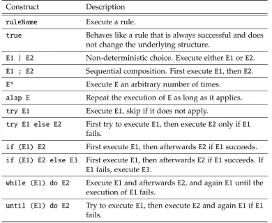
Algorithm 3.2 describes the execution algorithm for Henshin in pseudo-code. Henshin supports the passing of parameters between transformation units, but we omit this in the pseudo-code.

3.3. Term Rewriting

The next transformation language we discuss is called Stratego. It was developed by Visser [14] and is based on term rewriting. Instead of graphs, term-rewriting transformations useabstract syntax trees(AST) to represent the model. Abstract syntax trees consist ofterms, i.e. applicationsC(t1, . . . ,tn)of a constructor Cto termsti, lists,

strings or integers.

(35)

3.3. Term Rewriting 17

Algorithm 3.2Pseudo-code representation of Henshin’s execution algorithm.

1 Transformation transformationSystem 2

3 forall unit in transformationSystem : 4 processUnit ( unit )

5 6

7 function processUnit ( unit ): 8 if unit instanceof Rule :

9 Match match = unit . findMatch ()

10 if match != null :

11 unit . applyRule ( match )

12

13 else if unit instanceof IndependentUnit :

14 // Works in the same way as the

15 // basic graph transformation algorithm

16

17 else if unit instanceof PriorityUnit :

18 TransformationUnit nextUnit = unit . getNextSubUnit ()

19 boolean success = false

20 while nextUnit != null && ! success :

21 success = processUnit ( nextUnit )

22 nextUnit = unit . getNextSubUnit ()

23

24 else if unit instanceof SequentialUnit :

25 TransformationUnit nextUnit = unit . getNextSubUnit ()

26 boolean success = true

27 while nextUnit != null && success :

28 success = processUnit ( nextUnit )

29 nextUnit = unit . getNextSubUnit ()

30

31 else if unit instanceof CountedUnit : 32 int counter = unit . getCount ()

33 boolean success = true

34 while counter > 0 && success :

35 success = processUnit ( unit . getSubUnit () )

36 counter

--37

38 else if unit instanceof AmalgamationUnit :

39 Match kernelMatch = unit . getKernelRule () . findMatch ()

40 if kernelMatch != null :

41 if unit . getKernelRule () . applyRule ( kernelMatch ):

42 forall multiRule in unit . getMultiRules () :

43 forall match in multiRule . findMatch () :

44 multiRule . applyRule ( match )

45

46 else if unit instanceof ConditionalUnit :

47 boolean success = processUnit ( unit . getIf () )

48 if success :

49 processUnit ( unit . getThen () )

50 else if unit . getElse () != null :

(36)

[image:36.595.125.530.92.266.2]

Figure 3.2.: Henshin transformation units [3]

In Stratego the rule application strategy is specified explicitly using higher-order rewriting rules. That is, the developer can specify rules that combine other rules and execute them in a particular order.

Stratego has a number of language constructs to facilitate this, described in Table 3.2.

Algorithm 3.3 describes Stratego’s rule execution algorithm in pseudo-code. First a rule is matched against the source model and its variables are bound to specific terms. Afterwards any possible rule preconditions are checked and additional variables are bound. Finally the rule is applied, transforming the model.

Visser provides a number of transformation idioms to illustrate the rule application strategies that could be expressed using Stratego. We take a look at one of them, namely cascading transformation.

Cascading transformation is the most basic strategy for term rewriting (Algorithm 3.4). Small independent transformations are cumulatively applied in order to reach a desired result. The strategy tries to apply any of the rules, starting at the bottom of the abstract syntax tree. Each successful application restarts this process. If no rule can be applied, the algorithm moves to a higher level in the tree. This continues until we reach the root and there are no rules left that apply.

Listing 3.1 shows how this strategy can be expressed in Stratego notation. We first traverse the tree to get to the bottom level usingbottomup(s). We try to apply the sequence of rulesR1toRnuntil one of the rules succeeds. If a successful rule application

(37)

[image:37.595.57.456.112.515.2]

3.3. Term Rewriting 19

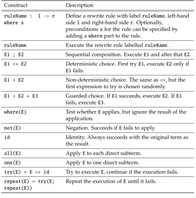
Table 3.2.: A selection of Stratego language constructs

Construct Description

ruleName : l -> r

where s

Define a rewrite rule with labelruleName, left-hand sideland right-hand sider. Optionally,

preconditionssfor the rule can be specified by adding awherepart to the rule.

ruleName Execute the rewrite rule labelledruleName.

E1 ; E2 Sequential composition. ExecuteE1and after thatE2.

E1 <+ E2 Deterministic choice. First tryE1, executeE2only if

E1fails.

E1 + E2 Non-deterministic choice. The same as<+, but the

first expression to try is chosen randomly.

E1 < E2 + E3 Guarded choice. IfE1succeeds, executeE2. IfE1

fails, executeE3.

where(E) Test whetherEapplies, but ignore the result of the

application.

not(E) Negation. Succeeds ifEfails to apply.

id Identity. Always succeeds with the original term as the result.

all(E) ApplyEto each direct subterm.

one(E) ApplyEto one direct subterm.

try(E) = E <+ id Try to executeE, continue if the execution fails.

repeat(E) = try(E; repeat(E))

Repeat the execution ofEuntil it fails.

Algorithm 3.3Pseudo-code representation of the Stratego rule application algorithm.

1 function applyRule ( Rule rule , AST tree ):

2 // check for match and collect variable bindings 3 Set bindings = rule .l. match ( tree )

4 // check extra preconditions 5 if rule .s != null :

6 Set precondition_bindings = rule .s. match ( tree ) 7 if rule .s == null || precondition_bindings != null :

8 bindings += precondition_bindings

9 if bindings != null :

10 // replace variables in term and replace tree

(38)

Algorithm 3.4 Pseudo-code representation of Stratego’s cascading transformation strategy.

1 // cascading transformations

2 function cascade ( Set rules , AST tree ): 3 // traverse bottom - up

4 forall child in tree . getChildren () :

5 cascade ( rules , child )

6

7 // try to apply rules

8 forall rule in rules :

9 if applyRule ( rule , tree ):

10 // successful application => start applying all

11 // rules again bottom - up

12 cascade ( rules , tree )

13 break

Listing 3.1: Cascading transformation expressed in the Stratego language. [14] 1 bottomup (s) = all ( bottomup (s)); s

2

3 innermost (s) = bottomup ( try (s; innermost (s))) 4

5 simplify = innermost ( R1 <+ ... <+ Rn )

3.4. ATL

The last transformation language we discuss in this chapter is ATL [13]. Although ATL is a hybrid language we only consider its declarative part here. As explained in Chapter 2, we use the imperative part for validation purposes in Chapter 4.

Declarative ATL has three kinds of transformation rules: matched,lazyand unique lazy.

Matched rules Matched rules match a specific type of source elements, possibly further restricted by a guard condition. A developer specifies the target elements that have to be created from these source elements, and how their properties should be initialized. Each source element may only be matched by a single matched rule.

ATL executes matched rules automatically in an arbitrary order. It also creates traceability links between source and target elements.

(39)

3.5. Analysis of Commonality and Variability 21

Unique lazy rules Unique lazy rules are lazy rules that are applied at most once for a specific match. If triggered more than once, they return the target elements that were already created earlier.

Algorithm 3.5 describes ATL’s transformation execution algorithm in pseudo-code. First, rules are matched and a list of matches is created. Second, the target elements are created. Last, the properties of the target elements are initialized.

Although we do not explicitly include the execution algorithm for (unique) lazy rules here, the algorithm for matched rules sans the matching can easily be reused for those kinds of rules.

3.5. Analysis of Commonality and Variability

Now that we have introduced the transformation execution algorithms of the various transformation languages, we proceed by analysing their commonalities and variabilit-ies. Looking at the execution of a model transformation, we can distinguish two levels at which the execution takes place: the rule level and the transformation level.

3.5.1. Rule Level

At the rule level we look at the operations that take place during rule execution. As we are considering declarative languages, developers do not explicitly specify most of these operations, i.e. they happen ‘behind the scenes’.

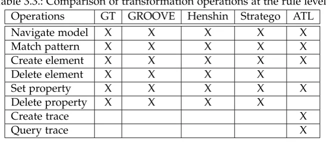
The transformation operations we identified are listed in Table 3.3. In every language the source model is navigated and elements from the source patterns are matched. Creating elements and setting properties is also something that every language is capable of.

In contrast, deleting elements or properties is not always possible. In ATL it is not possible to navigate the target model, and consequently it is not possible to delete parts of this model. Deletion of elements is possible when using ATL’srefining mode, but this mode can only be used if source and target models conform to the same metamodel. Moreover, some language features are disabled in this mode.

ATL does have two operations that are not available in other languages, namely for creating and querying a trace. Traces can be created in other languages, but are not supported natively in the implementation of these languages. Instead, they have to be specified explicitly in the transformation definition using a custom-made metamodel.

3.5.2. Transformation Level

At the transformation level we look at operations that make up a rule application strategy. The operations we identified are listed in Table 3.4.

(40)

Algorithm 3.5Pseudo-code representation of the ATL transformation algorithm.

1 Transformation transformation 2 InputModel inputModel

3 List matches

4 List targetElements 5 Dictionary traces 6

7 // match rules

8 forall rule in transformation . getMatchedRules () : 9 forall match in inputModel . getMatches ( rule ):

10 matches += match

11

12 // execute matched rules 13 forall match in matches : 14 // create target elements

15 forall t in match . getRule () . getTargets () : 16 Object target = new (t. getType () ) ()

17 targetElements += target

18 // create trace links

19 traces [ match . getSource () ] = target 20

21 // initialize target - element properties 22 forall target in targetElements :

23 forall property in target . getProperties () :

24 // if primitive , assign directly

25 if isPrimitive ( property . getContent () ):

26 target . setProperty ( property . getName () , property . getContent () )

27 else :

28 // if source element , resolve , then assign

29 Trace trace = traces [ property . getContent () ]

30 if trace != null :

31 target . setProperty ( property . getName () , trace ) 32

33 // if trace query , resolve , then assign

34 else if isQuery ( property . getContent () ):

35 Trace trace = traces [ property . getContent () . getSource () ] 36 target . setProperty ( property . getName () , trace )

37

38 // if target element , assign directly

39 else :

(41)

[image:41.595.105.432.99.241.2]

3.6. Conclusions 23

Table 3.3.: Comparison of transformation operations at the rule level. Operations GT GROOVE Henshin Stratego ATL

Navigate model X X X X X

Match pattern X X X X X

Create element X X X X X

Delete element X X X X

Set property X X X X X

Delete property X X X X

Create trace X

Query trace X

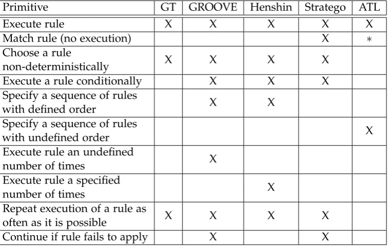
but not actually execute the rule. ATL is a special case: this feature is not available to developers, but is nonetheless an essential part of the language’s execution algorithm.

Other available operations are:

• Choosing a rule non-deterministically (i.e. randomly) from the available rules in a transformation.

• Executing a rule under the condition that a certain other rule does not apply.

• Executing a sequence of rules in some predefined order.

• Executing a sequence of rules in an undefined order. ATL’s execution algorithm works in this way: all matched rules are executed once for each match, in an undefined order.

• Executing a rule an undefined number of times.

• Executing a rule a specified number of times.

• Repeating the execution of a rule as long as possible. After executing the rule, we check whether or not the rule still applies. If so, we execute it again.

• Trying to execute a rule, but continue if it fails to apply. One of its uses is to stop recursion over a list once all elements have been processed, and continue the execution at a higher level.

3.6. Conclusions

(42)

[image:42.595.141.519.274.515.2]

Table 3.4.: Comparison of transformation operations at the transformation level.

Primitive GT GROOVE Henshin Stratego ATL

Execute rule X X X X X

Match rule (no execution) X ∗

Choose a rule

non-deterministically X X X X

Execute a rule conditionally X X X

Specify a sequence of rules

with defined order X X

Specify a sequence of rules

with undefined order X

Execute rule an undefined

number of times X

Execute rule a specified

number of times X

Repeat execution of a rule as

often as it is possible X X X X

(43)

4

Primitive Model Transformation Language

Using our observations discussed in the previous chapter, we can now define our own model transformation language, consisting of just a few primitive operations, in which all of the afore discussed transformation execution algorithms can be expressed.

4.1. Language Definition

4.1.1. Model Navigation Operations

First of all we need basic model navigation operations. The navigation operations available are quite dependent on the representation of the model in an actual im-plementation. Because the availability of such operations is not related to the way a transformation is executed, we assume that all operations necessary to navigate a model efficiently are available. Some example model navigation operations that are used in our primitive representations of the execution algorithms are described below.

transformation.getRules() Retrieve the rules in a transformation (graph transformation).

transformation.getSourceModel() Retrieve the source model of a transformation (graph transformation).

transformation.getTransformationUnits() Retrieve the transformation units in a trans-formation (Henshin).

transformation.getRules() Retrieve the rules in a transformation (Stratego).

rule.getTransformation() Retrieve the transformation to which a rule belongs (graph transformation).

(44)

rule.getTarget() Retrieve the target elements of a rule (graph transformation).

rule.getPreconditions() Retrieve the preconditions for a rule (Stratego).

unit.getSubUnits() Retrieve the subunits of a transformation unit (Henshin).

tree.getChildren() Retrieve the children of an AST element (Stratego).

4.1.2. Collection Operations

Second, we assume that basic operations to navigate and manipulate collections are also available. Some example collection operations that we use in our primitive representations of the execution algorithms are described below.

collection.add(element) Add an element as the last element of a collection.

collection.unshift() Add an element as the first element of a collection.

collection.shift() Remove the first element from a collection and return the element.

collection.remove(element) Remove an element from a collection.

collection.get(index) Retrieve the element at the specified index of a collection.

collection.contains(element) Check if a collection contains an element. Returns a boolean.

collection.copy() Returns a deep copy of a collection.

4.1.3. Logical and Arithmetic Operations

Third, we assume support for basic logical and arithmetic operations. Some examples of these operations are:

== Equals

!= Not equal to

> Greater than

< Less than

= Assignment

+ Addition

- Subtraction ∗ Multiplication

/ Division

4.1.4. Functions

Fourth, we assume that functions are supported. Strictly speaking, functions are not primitives, but we use them to structure the algorithms and to enable recursion. Functions can have parameters that pass references. A function does not return any value. A function namedmyFunctionwith a parameter namedparameter1and type

TypeXcan be specified as follows:

(45)

4.1. Language Definition 27

4.1.5. Exception Handling

Fifth, we have exception handling. This was not observed in any of the selected transformation algorithms, but can be useful to convey information about errors during the transformation execution. An exception is raised using raise(). The

raiseprimitive is never applicable and thus causes the execution to return to a higher

level. The exception can be caught usingcatch(), which is applicable if the specified exception has been raised and was not yet caught.

4.1.6. Transformation-level Operations

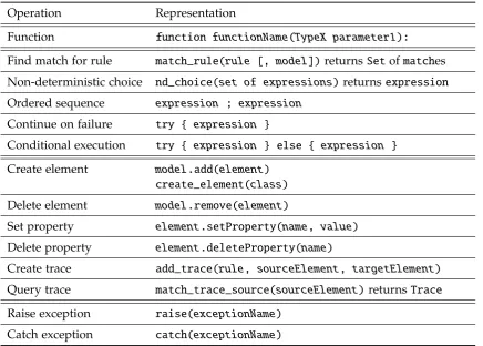
The primitive transformation operations are summarized in Table 4.1. We discuss them one by one.

Find match for rule match_rule(rule[, model])returnsSetofmatches

Searches the source model for elements that match the left-hand side of the specified rule. It returns a set of matches. If the model parameter is provided, the specified (sub)model is searched instead of the source model.

We do not define the search algorithm that is used to search the model. The choice of search algorithm is left to the implementers of the primitive language.

Non-deterministic choice nd_choice(set of expressions)returnsexpression

Chooses one element of the set of expressions at random and returns the element. An expression can be an operation, a call to a function or a literal value (eg. 42).

Ordered sequence expression ; expression

Executes the expressions in the defined order. If the first expression fails to execute, the second will not be executed.

Continue on failure try { expression }

Tries to execute the expression. If it fails, continue as if the execution was successful.

Conditional execution try { expression } else { expression }

Tries to execute the first expression. If it fails, try to execute the second expression.

4.1.7. Rule-level Operations

Create element model.add(element) create_element(class)

The first operation (add) adds an element to a model. This is used in algorithms that make copies of target elements and include the copies in the target model.

(46)

Delete element model.remove(element)

Deletes an element from a model.

Set property element.setProperty(name, value)

Sets the value of the property ‘name’ on the element to ‘value’.

Delete property element.deleteProperty(name)

Deletes (or nullifies) the property ‘name’ on the element.

Create trace add_trace(rule, sourceElement, targetElement)

Creates a trace that connects the source element to the target element in the context of a rule.

Query trace match_trace_source(sourceElement)returnsTrace

Looks for a trace with the specified source element and returns it. The execution of this operation fails if no trace is found. ATraceobject contains a reference to a rule, a source element and a target element.

4.1.8. Operations not included

Some of the operations observed earlier are not included in our primitive language:

• Execute a rule. This is a primitive operation at the transformation level, but one that is tied closely to the execution algorithm that is used. For example, in graph transformation, rules are executed on a per-rule basis, while in ATL the execution is split into three phases (match, create, initialize) and all rules have to be processed before the next phase is started. Therefore we cannot provide a single language construct that can be used in all algorithms.

• Execute rule an undefined number of times. This operation is only present in GROOVE and was most likely added to the language because of its roots in defining automata. We see no practical use for this operation in a general-purpose transformation language and it can be emulated with the other primitives anyway.

• Execute a rule a specified number of times. This is another operation that can be emulated using the other primitives on a per-algorithm basis, for example:

function for ( Rule r , int n):

try { n > 0 ; executeRule (r) ; for (r , n -1) } else { n == 0 }

In this exampleexecuteRule()is the function the algorithm in question uses to execute a transformation rule.

(47)

[image:47.595.59.496.107.419.2]

4.2. Application of the Primitive Language 29

Table 4.1.: Primitive transformation language operations

Operation Representation

Function function functionName(TypeX parameter1):

Find match for rule match_rule(rule [, model])returnsSetofmatches

Non-deterministic choice nd_choice(set of expressions)returnsexpression

Ordered sequence expression ; expression

Continue on failure try { expression }

Conditional execution try { expression } else { expression }

Create element model.add(element)

create_element(class)

Delete element model.remove(element)

Set property element.setProperty(name, value)

Delete property element.deleteProperty(name)

Create trace add_trace(rule, sourceElement, targetElement)

Raise exception raise(exceptionName)

Catch exception catch(exceptionName)

function repeat ( Rule r): try { executeRule (r) ; repeat (r) }

• Specify a sequence of rules with undefined order. This can be emulated by choosing rules non-deterministically and removing them from a set (or from the transformation model) once they have been executed.

4.2. Application of the Primitive Language

We have defined our primitive model transformation language for specifying trans-formation algorithms, and we now express all of the aforediscussed algorithms using our own language.

4.2.1. Graph Transformation

(48)

First, we select an arbitrary transformation rule (PL line 11, PC line 8). We search for all occurrences of the rule’s left-hand side in the source model (PL line 12, PC line 10) and select an arbitrary match (PL line 14, PC line 10).

We execute the rule with this match (PL lines 22-30, PC lines 11-25). We remove all matched source elements that do not exist in the rule’s right-hand side (PL line 26, PC lines 12-14). We add the elements that exist in rule’s right-hand side but not in the rule’s left-hand side (PL line 28, PC lines 21-23). Finally, we restart the transformation (PL line 5, PC lines 25-29).

If no match is found for a rule, we try matching another rule (PL lines 15-19, PC lines 8-10). When no rule matches, the transformation is complete (PL lines 3-6, PC lines 31-33).

4.2.2. Henshin

An implementation of Henshin’s execution algorithm in our primitive language is included in Appendix A.2. This implementation reuses theexecuteRule()function from the graph transformation algorithm implementation. Again we compare this implementation (PL) to the pseudo-code version (PC) described in Algorithm 3.2 in Chapter 3.

We process all transformation units that are subunits of theTransformationone at a time (PL lines 6-8, PC lines 3-4).

• If the unit is a Rule, we look for a match in the source model and execute the

Rule if one is found (PL lines 12-15, PC lines 8-11).

• If the unit is an IndependentUnit, we execute its subunits using the graph transformation algorithm (PL lines 17-9, 46-63; PC lines 13-15).

• If the unit is aPriorityUnit, we execute its subunits according to their priorities (PL lines 21-23, 65-73; PC lines 17-22).

• If the unit is aSequentialUnit, we execute its subunits in the predefined sequence (PL lines 25-27, 75-82; PC lines 24-29).

• If the unit is aCountedUnit, we execute its subunits the specified number of times (PL lines 30-31, 84-91; PC lines 31-36).

• If the unit is an AmalgamationUnit, we first try to find a match for the kernel rule (PL lines 33-35, 93-94; PL lines 38-41). If a match is found, we try to find matches for themulti-rulesand execute them (PL lines 95-101, PC lines 42-44).

• If the unit is aConditionalUnit, we first try to execute theifsubunit (PL lines 37-38, 103-105; PC lines 46-47). If the execution of ifsucceeds, we execute thethen

(49)

4.2. Application of the Primitive Language 31

4.2.3. Term Rewriting

An implementation of Stratego’s cascading transformation strategy in our primitive lan-guage (PL) is included in Appendix A.3. The pseudo-code version (PC) was described in Algorithm 3.4 in Chapter 3.

To start, we traverse the AST to get to the bottom level (PL lines 4-6, PC lines 2-5). We try to execute the first rule in the list (PL lines 7-13, PC lines 8-9) and continue with the next rule if the first fails to execute (PL lines 16-20, PC lines 8-9). Once a successful rule execution has taken place, we restart the transformation on the current subtree (PL lines 14-15, PC lines 12-13). When no executable rules remain we move to the next level of the tree (PL lines 6-8, PC lines 4-5).

The execution of a rule was described in Algorithm 3.3 in Chapter 3. We look for matches of the left-hand side of the rule in the source model (PL line 25, PC line 3). We bind its variables to the source elements that matched (PL line 26, PC line 3). If appropriate, we check if the rule’s preconditions match and bind additional variables to source elements (PL lines 27-32, PC lines 5-8). Finally, we replace the bound source elements by their respective target elements from the right-hand side of the rule (PL line 33, PC lines 9-11).

4.2.4. Declarative ATL

An implementation of the declarative ATL algorithm in our primitive language (PL) is included in Appendix A.4. The pseudo-code version (PC) was described in Al-gorithm 3.5 in Chapter 3.

The execution consists of three phases. First, we match the left-hand side of all rules to elements in the source model and save the matches using traces (PL lines 2, 6-15, 37-45; PC lines 7-10). Second, we create the right-hand side elements of the rule in the target model (PL lines 3, 17-25, 47-57; PC lines 12-19). Third, we initialize the properties of the target elements we just created (PL lines 4, 27-35, 59-94; PC lines 22-40).

4.2.5. Imperative ATL

We use the imperative ATL algorithm to validate that our primitive pseudo language can indeed express other kinds of transformation languages that were not considered while defining our language.

Imperative ATL uses called rules instead of matched rules. Called rules are not executed automatically, they must be called explicitly from another rule. Instead of defining the left-hand side and right-hand side of a rule, one defines a right-hand side and a ‘dosection’. Thedosection can contain imperative statements, namely:

• A call to a another called rule or lazy (unique) rule. Parameters can be passed to the called rule.

• An assignment statement target <- expression that assigns the result of an

(50)

• A conditonal statement: if( condition ) { statements1 } else { statements2 }

• An iteration statement that iterates over a collection, executing statements one time for each element of the collection assigned toiterator:

for(iterator in collection) { statements }

An implementation of the imperative ATL algorithm in our primitive language is included in Appendix A.5. An imperative ATL transformation starts at the entry point rule(line 2). When a called rule is executed, we first create the target elements and initialize their properties (lines 6-8). Second, all statements in thedosection are executed (line 10-55). If another rule is a called, we execute this rule with the passed parameters (lines 17-18). For assignment statements we evaluate the expression and assign its result to the specified module property (lines 22-23).

For conditional statements we first evaluate the condition (lines 27-29). If the condi-tion is true, we execute the first group of statements (line 31). If not, we execute the second group of statements (lines 32-34).

For iteration statements we iterate over the provided collection, adding the first element of the collection to the execution context of the enclosed statements each time (lines 37-55).

It should be noted that our implementation reuses some of the functions of our declarative ATL implementation. Additionally, the official ATL implementation does not create traces when executing imperative ATL. Our implementation does create traces, because it enables us to reuse part of the declarative algorithm. We consider this an implementation detail.

4.3. Related Work

Syriani and Vangheluwe [23] have conducted a similar deconstruction of transform-ation languages into primitives. Their primitives are objects (for instance aMatcher,

Rewriter,Iterator) that perform parts of the transformation and exchange messages.

A rough comparison between their and our primitives can be found in Table 4.2. Unfortunately, they do not motivate their choice of primitives.

Syriani and Vangheluwe do include support for parallel processing, an aspect of model transformation that we do not deal with in this thesis.

Our language includes primitives for creating and querying traces, while they do not provide support for tracing in their language.

4.4. Conclusions

(51)

[image:51.595.77.458.109.303.2]

4.4. Conclusions 33

Table 4.2.: Comparison of transformation primitives

Syriani and Vangheluwe [23] Our primitives

Matcher Match rule

Rewriter Create/delete element, set/delete property

Iterator Conditional execution, functions

Resolver Conditional execution, exception handling

Rollbacker Continue on failure

Selector Non-deterministic choice

Synchronizer

Composer Ordered sequence

Create/query trace

(52)

(53)

5

Transforming Model Transformations

Having defined our own primitive transformation language in Chapter 4, we can build a transformation framework that can actually transform models using transformation execution specifications written in this language.

5.1. Architecture

As mentioned before, model transformations can be described using the pattern shown in Figure 5.1. We have a source model Ma, a target model Mband a transformation

definitionTab. The transformation definition is written in a transformation language TL. When executed, the transformation engine runsTab, which transforms Ma to Mb.

Our transformation engine architecture is shown in Figure 5.2. Instead of interpreting

T_ab directly, we use it as input model for transformation T_pl. T_pl is a transformation written in our primitive languagePL. It contains rules for interpretingTL transforma-tions.

T_plitself is interpreted by our primitive language interpreter I_pl.

Since the transformation language is itself implemented as a transformation, it is relatively easy to add support for new languages and extend existing languages.

5.2. Interpreter Implementation

The transformation engine is implemented as a plug-in for the Eclipse platform [24]. This gives us access to the Eclipse Modeling Framework [5] and related libraries.

Though the syntax ofPL as described in Chapter 4 works fine for defining trans-formation languages, it became clear switching to a more established syntax would ease the implementation of thePL interpreter significantly. Implementing the Chapter

(54)

[image:54.595.193.463.102.323.2]

Figure 5.1.: Model Transformation Pattern

[image:54.595.193.466.387.633.2]

(55)

5.3. Transformation Language Implementation 37

ThrTrace rule: String

[image:55.595.218.320.94.151.2]

source: List<EObject> target: List<EObject>

Figure 5.3.: Thrascias Trace structure

4 syntax would mean implementing our own OCL [8] engine, which is required for model navigation and collection operations. This is not a small task and out of scope for this thesis.

We decided to use a syntax based onMistral[9], a general purpose model transform-ation language and to use its implementtransform-ation of OCL. We use only a small subset of Mistral’s syntax, which is much more elaborate. Our implementation is calledThrascias.

Thrascias’ abstract syntax (MM_pl) is defined as an ECore model, shown in Figure 5.4. The concrete syntax is described in Table 5.1. It comprises OCL for expressions, operations for defining which models are used, a function definition and the primitive operations described in Chapter 4. In addition to the input and output models, two other metamodels are always present: the EMF metamodelEcoreandThrascias. The Thrascias metamodel contains the Trace class which the interpreter uses for managing traces. The structure of this class is shown in Figure 5.3.

For reflective purposes, the model of the transformation currently being executed is accessible as_Transformation_.

We map the concrete syntax to the abstract syntax using EMFText [25]. It also provides an editor and syntax checker for the language. The interpreter itself is implemented as a standard interpreter pattern with a stack.

5.3. Transformation Language Implementation

We implement two of the analysed transformation languages in our framework: graph transformation and ATL. The implementation of the other languages is left as further work. The implementations are included in Appendix B.1 and Appendix B.2.

(56)

Figur

e

5.4.

:

Thrascias

abstract

[image:56.595.202.463.82.699.2]

(57)

[image:57.595.55.521.153.631.2]

5.3. Transformation Language Implementation 39

Table 5.1.: Thrascias operations

Operation Representation

Define transformation transform transformationName

Specify input model inputModel modelName: metamodelName

Specify output model outputModel modelName: metamodelName

Function functionName ModelElementRule {

source [parameter1: TypeX]

target [result1: TypeY = expression]

}

Model navigation OCL and Ecore

Collection operations OCL

Find match for element in set match(element, elementSet)returns

Sequence(Set(OclAny))

Non-deterministic choice collection->any(true)

Ordered sequence expression and expression

Conditional execution expression or expression

if expr then expr else expr endif

Continue on failure UsingModelElementRule

Create element create_element(eClass)

Delete element delete element

Set property update element {property=value}

Delete property update element {delete property}

Create trace add_trace(rule, [sourceElements[,

targetElements]])

Raise exception raise(exception)

(58)

5.4. Conclusions

(59)

6

Model Transformation Scenarios

We validate our implementation by executing two different model transformation scenarios, namely transforming object-oriented classes to relation tables and pulling up subclass attributes to a superclass. First, we implement the model transformations using SimpleGT and declarative ATL. Second, we execute these implementations with both their original interpreter and our own transformation framework. Third, we compare the results of the executions.

6.1. Common Use Cases

The use cases in which model transformations are most commonly applied can be categorized into five scenarios [11]:

• Generating lower-level models and source code from higher-level models

• Reverse engineering higher-level models from lower-level models or source code

• Generating views from a model using a query

• Mapping and synchronizing models

• Model evolution or refactoring

The first three scenarios usually involve generating and parsing source code files or other documents without an explicit metamodel. Because our research focuses on model-to-model transformations, we validate our implementation using the last two scenarios.

(60)

name : String

NamedElt

isAbstract : boolean

Classifier Class DataType

multivalued : boolean

Attribute 1 attr * * type 1 super * sub *

(a) Object-oriented class

-name : String Named

Table Column

0..1 key *

1 col * Type * type 1

(b) Relational table

Figure 6.1.: Metamodels for mapping scenario [4]

6.2. Object-oriented Class to Relational Table

For the model mapping use case, we choose one of the classic examples of model transformation: the mapping of an object-oriented class diagram to a relational database table model.

6.2.1. Implementation

Both models are shown in Figure 6.1. In the class metamodel (Figure 6.1a) aClasshas a name (inherited from the abstractNamedElt) and a number of Attributes. These

Attributesmay bemultivalued.Classinherits fromClassifier, which allows us to

declare thetypeofAttributes.

In the table metamodel (Figure 6.1b) aTablehas a name (inherited from the abstract

Named) and a number of Columns and keys. A Column has a Type and belongs to a

Table(itsowner) and might be akey ofanotherTable.

The implementations of this transformation in SimpleGT and declarative ATL are included in Appendix C.

6.2.2. Results

(61)

[image:61.595.89.448.85.343.2]

6.2. Object-oriented Class to Relational Table 43

Figure 6.2.: EMF ‘extlibrary’ metamodel (adapted from [5])

[image:61.595.87.448.382.649.2]

(62)

MySecondSubClass eSuperTypes: List eAttributes: List myAttribute: int MySuperClass eSuperTypes: List eAttributes: List MyFirstSubClass eSuperTypes: List eAttributes: List myAttribute: int

(a) Before transformation

MySecondSubClass eSuperTypes: List eAttributes: List MySuperClass eSuperTypes: List eAttributes: List myAttribute: int MyFirstSubClass eSuperTypes: List eAttributes: List

[image:62.595.113.563.93.235.2]

(b) After transformation

Figure 6.4.: Model for refactoring scenario

6.3. Pull Up Class Attribute to Superclass

For the second use case, model refactoring, we choose to refactor an object oriented class hierarchy. We take an attribute that is present on all subclasses of a certain class and move the attribute to the superclass. This is also known as ‘pulling up’ a class attribute.

6.3.1. Implementation

We move an attribute called myAttributefrom a class to its superclass (Figure 6.4). The model conforms to the Ecore metamodel. Prerequisite for this refactoring is an attribute which is present in all subclasses of a certain superclass, and is not present in the superclass itself.

The implementations of this transformation in SimpleGT and declarative ATL are included in Appendix D.

6.3.2. Results

Again we apply the transformations to our example book library model (Figure 6.2). We move the attributesname of all the subclasses ofPersonto their superclass. The result of the transformation is shown in Figure 6.3. Verifying the results manually, we find no differences in transformation result between the original interpreters of SimpleGT or ATL and our own implementations.

6.4. Conclusions

(63)

6.4. Conclusions 45

an example model using both the original interpreters and our own implementations. In our manual verification we found no difference in transformation result.

(64)

(65)

7

Conclusions and Future Work

In Chapter 1 we introduced the problem of having many different model transformation languages, all with their own unique approach. We recognized that, despite their differences, they have some features in common. We asked the question: “how can we execute different model transformation languages in a common environment, while retaining the variability between the languages?”. We can now answer this question based on our research.

7.1. What should a common execution environment for model

transformation languages look like?

In Chapter 2 we explored models and model transformations. We categorized transform-ation languages based on properties like transformtransform-ation approach and rule applictransform-ation strategy. Using this categorization, we selected five significantly different transform-ation languages for further investigtransform-ation: graph transformtransform-ation, GROOVE, Henshin, Stratego and declarative ATL.

In Chapter 3 we took a closer look at the execution algorithms of the selected languages. We analysed the commonality and variability between them, both at the rule level and the transformation level.

In Chapter 4 we defined our own primitive model transformation language based on the analysis of commonality and variability. We expressed the execution algorithms for all analysed languages in our primitive language.

Subsequently, we took a look at imperative ATL. It has a completely different transformation approach, one not considered during the design of our primitive language. Nevertheless we were able to express its execution algorithm, demonstrating

Towards a Unifying Framework for Modelling and Executing Model Transformations

MASTER’S THESIS