Neural CRF Parsing
Greg Durrett and Dan Klein Computer Science Division University of California, Berkeley
{gdurrett,klein}@cs.berkeley.edu
Abstract
This paper describes a parsing model that combines the exact dynamic programming of CRF parsing with the rich nonlinear fea-turization of neural net approaches. Our model is structurally a CRF that factors over anchored rule productions, but in-stead of linear potential functions based on sparse features, we use nonlinear po-tentials computed via a feedforward neu-ral network. Because potentials are still local to anchored rules, structured infer-ence (CKY) is unchanged from the sparse case. Computing gradients during learn-ing involves backpropagatlearn-ing an error sig-nal formed from standard CRF sufficient statistics (expected rule counts). Us-ing only dense features, our neural CRF already exceeds a strong baseline CRF model (Hall et al., 2014). In combination with sparse features, our system1achieves
91.1 F1 on section 23 of the Penn Tree-bank, and more generally outperforms the best prior single parser results on a range of languages.
1 Introduction
Neural network-based approaches to structured NLP tasks have both strengths and weaknesses when compared to more conventional models, such conditional random fields (CRFs). A key strength of neural approaches is their ability to learn nonlinear interactions between underlying features. In the case of unstructured output spaces, this capability has led to gains in problems rang-ing from syntax (Chen and Mannrang-ing, 2014; Be-linkov et al., 2014) to lexical semantics (Kalch-brenner et al., 2014; Kim, 2014). Neural methods are also powerful tools in the case of structured 1System available at http://nlp.cs.berkeley.edu
output spaces. Here, past work has often relied on recurrent architectures (Henderson, 2003; Socher et al., 2013; ˙Irsoy and Cardie, 2014), which can propagate information through structure via real-valued hidden state, but as a result do not admit ef-ficient dynamic programming (Socher et al., 2013; Le and Zuidema, 2014). However, there is a nat-ural marriage of nonlinear induced features and efficient structured inference, as explored by Col-lobert et al. (2011) for the case of sequence mod-eling: feedforward neural networks can be used to score local decisions which are then “reconciled” in a discrete structured modeling framework, al-lowing inference via dynamic programming.
In this work, we present a CRF constituency parser based on these principles, where individ-ual anchored rule productions are scored based on nonlinear features computed with a feedfor-ward neural network. A separate, identically-parameterized replicate of the network exists for each possible span and split point. As input, it takes vector representations of words at the split point and span boundaries; it then outputs scores for anchored rules applied to that span and split point. These scores can be thought of as non-linear potentials analogous to non-linear potentials in conventional CRFs. Crucially, while the network replicates are connected in a unified model, their computations factor along the same substructures as in standard CRFs.
Prior work on parsing using neural network models has often sidestepped the problem of struc-tured inference by making sequential decisions (Henderson, 2003; Chen and Manning, 2014; Tsuboi, 2014) or by doing reranking (Socher et al., 2013; Le and Zuidema, 2014); by contrast, our framework permits exact inference via CKY, since the model’s structured interactions are purely dis-crete and do not involve continuous hidden state. Therefore, we can exploit a neural net’s capac-ity to learn nonlinear features without modifying
S
NP VP
DT NNP VBZ NP
… W
The Fed issued
Structured inference (discrete) Feature extraction (continuous)
fo
h
fw
v(fw)
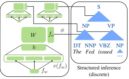
Figure 1: Neural CRF model. On the right, each anchored rule (r, s) in the tree is independently scored by a function φ, so we can perform in-ference with CKY to compute marginals or the Viterbi tree. On the left, we show the process for scoring an anchored rule with neural features: words infw(see Figure 2) are embedded, then fed through a neural network with one hidden layer to compute dense intermediate features, whose con-junctions with sparse rule indicator featuresfoare scored according to parametersW.
our core inference mechanism, allowing us to use tricks like coarse pruning that make inference ef-ficient in the purely sparse model. Our model can be trained by gradient descent exactly as in a con-ventional CRF, with the gradient of the network parameters naturally computed by backpropagat-ing a difference of expected anchored rule counts through the network for each span and split point. Using dense learned features alone, the neu-ral CRF model obtains high performance, out-performing the CRF parser of Hall et al. (2014). When sparse indicators are used in addition, the resulting model gets 91.1 F1 on section 23 of the Penn Treebank, outperforming the parser of Socher et al. (2013) as well as the Berkeley Parser (Petrov and Klein, 2007) and matching the dis-criminative parser of Carreras et al. (2008). The model also obtains the best single parser results on nine other languages, again outperforming the system of Hall et al. (2014).
[image:2.595.73.291.65.199.2]2 Model
Figure 1 shows our neural CRF model. The model decomposes over anchored rules, and it scores each of these with a potential function; in a standard CRF, these potentials are typically lin-ear functions of sparse indicator features, whereas
reflected the flip side of the Stoltzman personality .
reflected the side of personality .
i j k
[[PreviousWord = reflected]], [[SpanLength = 7]], … fs
NP PP
NP
r=NP NP PP!
fw
v(fw)
Figure 2: Example of an anchored rule production for the rule NP→NP PP. From the anchorings= (i, j, k), we extract either sparse surface features fsor a sequence of word indicatorsfw which are embedded to form a vector representation v(fw) of the anchoring’s lexical properties.
in our approach they are nonlinear functions of word embeddings.2 Section 2.1 describes our
no-tation for anchored rules, and Section 2.2 talks about how they are scored. We then discuss spe-cific choices of our featurization (Section 2.3) and the backbone grammar used for structured infer-ence (Section 2.4).
2.1 Anchored Rules
The fundamental units that our parsing models consider are anchored rules. As shown in Fig-ure 2, we define an anchored rule as a tuple(r, s), where r is an indicator of the rule’s identity and s = (i, j, k) indicates the span (i, k) and split pointj of the rule.3 A treeT is simply a
collec-tion of anchored rules subject to the constraint that those rules form a tree. All of our parsing models are CRFs that decompose over anchored rule pro-ductions and place a probability distribution over trees conditioned on a sentencewas follows:
P(T|w)∝exp
X
(r,s)∈T
φ(w, r, s)
2Throughout this work, we will primarily consider two
potential functions: linear functions of sparse indicators and nonlinear neural networks over dense, continuous features. Although other modeling choices are possible, these two points in the design space reflect common choices in NLP, and past work has suggested that nonlinear functions of indi-cators or linear functions of dense features may perform less well (Wang and Manning, 2013).
3For simplicity of exposition, we ignore unary rules;
[image:2.595.308.527.69.198.2]where φ is a scoring function that considers the input sentence and the anchored rule in question. Figure 1 shows this scoring process schematically. As we will see, the module on the left can be be a neural net, a linear function of surface features, or a combination of the two, as long as it provides anchored rule scores, and the structured inference component is the same regardless (CKY).
A PCFG estimated with maximum likelihood hasφ(w, r, s) = logP(r|parent(r)), which is in-dependent of the anchoringsand the wordsw ex-cept for preterminal productions; a basic discrimi-native parser might let this be a learned parameter but still disregard the surface information. How-ever, surface features can capture useful syntactic cues (Finkel et al., 2008; Hall et al., 2014). Con-sider the example in Figure 2: the proposed parent NP is preceded by the wordreflectedand followed by a period, which is a surface context character-istic of NPs or PPs in object position. Beginning with the and ending with personality are typical properties of NPs as well, and the choice of the particular rule NP → NP PP is supported by the fact that the proposed child PP begins withof. This information can be captured with sparse features (fs in Figure 2) or, as we describe below, with a neural network taking lexical context as input. 2.2 Scoring Anchored Rules
Following Hall et al. (2014), our baseline sparse scoring function takes the following bilinear form:
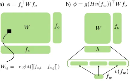
φsparse(w, r, s;W) =fs(w, s)>W fo(r)
where fo(r) ∈ {0,1}no is a sparse vector of features expressing properties of r (such as the rule’s identity or its parent label) andfs(w, s) ∈
{0,1}ns is a sparse vector of surface features as-sociated with the words in the sentence and the anchoring, as shown in Figure 2. W is ans×no matrix of weights.4 The scoring of a particular
an-chored rule is depicted in Figure 3a; note that sur-face features and rule indicators are conjoined in a systematic way.
The role offs can be equally well played by a vector of dense features learned via a neural net-4A more conventional expression of the scoring function
for a CRF isφ(w, r, s) = θ>f(w, r, s), with a vectorθfor
the parameters and a single feature extractorf that jointly inspects the surface and the rule. However, when the feature representation conjoins each rulerwith surface properties of the sentence in a systematic way (an assumption that holds in our case as well as for standard CRF models for POS tagging and NER), this is equivalent to our formalism.
fo
W W fo
fs
Wij= weight([[fs,i^fo,j]])
a) b)
fw
v(fw)
h =f>
s W fo =g(Hv(fw))>W fo
Figure 3: Our sparse (left) and neural (right) scor-ing functions for CRF parsscor-ing. fs and fw are raw surface feature vectors for the sparse and neu-ral models (respectively) extracted over anchored spans with split points. (a) In the sparse case, we multiply fs by a weight matrix W and then a sparse output vectorfoto score the rule produc-tion. (b) In the neural case, we first embedfw and then transform it with a one-layer neural network in order to produce an intermediate feature repre-sentationhbefore combining withW andfo.
work. We will now describe how to compute these features, which represent a transformation of sur-face lexical indicatorsfw. Definefw(w, s)∈Nnw to be a function that produces a fixed-length se-quence of word indicators based on the input sen-tence and the anchoring. This vector of word identities is then passed to an embedding function v : N → Rne and the dense representations of the words are subsequently concatenated to form a vector we denote by v(fw).5 Finally, we mul-tiply this by a matrix H ∈ Rnh×(nwne) of real-valued parameters and pass it through an elemen-twise nonlinearity g(·). We use rectified linear units g(x) = max(x,0) and discuss this choice more in Section 6.
Replacingfswith the end result of this compu-tationh(w, s;H) = g(Hv(fw(w, s))), our scor-ing function becomes
φneural(w, r, s;H, W) =h(w, s;H)>W fo(r) as shown in Figure 3b. For a fixedH, this model can be viewed as a basic CRF with dense input fea-tures. By learningH, we learn intermediate fea-ture representations that provide the model with 5Embedding words allows us to use standard pre-trained
more discriminating power. Also note that it is possible to use deeper networks or more sophis-ticated architectures here; we will return to this in Section 6.
Our two models can be easily combined:
φ(w, r, s;W1, H, W2) =φsparse(w, r, s;W1)
+φneural(w, r, s;H, W2)
Weights for each component of the scoring func-tion can be learned fully jointly and inference pro-ceeds as before.
2.3 Features
We take fs to be the set of features described in Hall et al. (2014). At the preterminal layer, the model considers prefixes and suffixes up to length 5 of the current word and neighboring words, as well as the words’ identities. For nonterminal pro-ductions, we fire indicators on the words6 before
and after the start, end, and split point of the an-chored rule (as shown in Figure 2) as well as on two other span properties, span length and span shape (an indicator of where capitalized words, numbers, and punctuation occur in the span).
For our neural model, we take fw for all pro-ductions (preterminal and nonterminal) to be the words surrounding the beginning and end of a span and the split point, as shown in Figure 2; in partic-ular, we look two words in either direction around each point of interest, meaning the neural net takes 12 words as input.7 For our word embeddingsv,
we use pre-trained word vectors from Bansal et al. (2014). We compare with other sources of word vectors in Section 5. Contrary to standard practice, we do not update these vectors during training; we found that doing so did not provide an accuracy benefit and slowed down training considerably. 2.4 Grammar Refinements
A recurring issue in discriminative constituency parsing is the granularity of annotation in the base grammar (Finkel et al., 2008; Petrov and Klein, 2008; Hall et al., 2014). Using finer-grained sym-bols in our rulesrgives the model greater capacity, but also introduces more parameters intoW and 6The model actually uses the longest suffix of each word
occurring at least 100 times in the training set, up to the entire word. Removing this abstraction of rare words harms perfor-mance.
7The sparse model did not benefit from using this larger
neighborhood, so improvements from the neural net are not simply due to considering more lexical context.
increases the ability to overfit. Following Hall et al. (2014), we use grammars with very little anno-tation: we use no horizontal Markovization for any of experiments, and all of our English experiments with the neural CRF use no vertical Markovization (V = 0). This also has the benefit of making the system much faster, due to the smaller state space for dynamic programming. We do find that using parent annotation (V = 1) is useful on other lan-guages (see Section 7.2), but this is the only gram-mar refinement we consider.
3 Learning
To learn weights for our neural model, we maxi-mize the conditional log likelihood of ourD train-ing treesT∗:
L(H, W) =XD
i=1
logP(Ti∗|wi;H, W)
Because we are using rectified linear units as our nonlinearity, our objective is not everywhere dif-ferentiable. The interaction of the parameters and the nonlinearity also makes the objective non-convex. However, in spite of this, we can still fol-low subgradients to optimize this objective, as is standard practice.
Recall thath(w, s;H)are the hidden layer ac-tivations. The gradient of W takes the standard form of log-linear models:
∂L
∂W =
X
(r,s)∈T∗
h(w, s;H)fo(r)> −
X
T
P(T|w;H, W) X
(r,s)∈T
h(w, s;H)fo(r)>
Note that the outer products give matrices of fea-ture counts isomorphic toW. The second expres-sion can be simplified to be in terms of expected feature counts. To update H, we use standard backpropagation by first computing:
∂L
∂h =
X
(r,s)∈T∗
W fo(r) −
X
T
P(T|w;H, W) X
(r,s)∈T
W fo(r)
Learning uses Adadelta (Zeiler, 2012), which has been employed in past work (Kim, 2014). We found that Adagrad (Duchi et al., 2011) performed equally well with tuned regularization and step size parameters, but Adadelta worked better out of the box. We set the momentum termρ = 0.95
(as suggested by Zeiler (2012)) and did not reg-ularize the weights at all. We used a minibatch size of 200 trees, although the system was not par-ticularly sensitive to this. For each treebank, we trained for either 10 passes through the treebank or 1000 minibatches, whichever is shorter.
We initialized the output weight matrix W to zero. To break symmetry, the lower level neural network parameters H were initialized with each entry being independently sampled from a Gaus-sian with mean 0 and variance 0.01; GausGaus-sian per-formed better than uniform initialization, but the variance was not important.
4 Inference
Our baseline and neural model both score an-chored rule productions. We can use CKY in the standard fashion to compute either expected an-chored rule counts EP(T|w)[(r, s)] or the Viterbi treearg maxTP(T|w).
We speed up inference by using a coarse prun-ing pass. We follow Hall et al. (2014) and prune according to an X-bar grammar with head-outward binarization, ruling out any constituent whose max marginal probability is less thane−9. With this pruning, the number of spans and split points to be considered is greatly reduced; how-ever, we still need to compute the neural network activations for each remaining span and split point, of which there may be thousands for a given sen-tence.8 We can improve efficiency further by
not-ing that the same word will appear in the same po-sition in a large number of span/split point combi-nations, and cache the contribution to the hidden layer caused by that word (Chen and Manning, 2014). Computing the hidden layer then simply requires addingnw vectors together and applying the nonlinearity, instead of a more costly matrix multiply.
Because the number of rule indicators no is fairly large (approximately 4000 in the Penn Tree-bank), the multiplication byW in the model is also 8One reason we did not choose to include the rule identity
foas an input to the network is that it requires computing an even larger number of network activations, since we cannot reuse them across rules over the same span and split point.
expensive. However, because only a small number of rules can apply to a given span and split point, fo is sparse and we can selectively compute the terms necessary for the final bilinear product.
Our combined sparse and neural model trains on the Penn Treebank in 24 hours on a single machine with a parallelized CPU implementation. For ref-erence, the purely sparse model with a parent-annotated grammar (necessary for the best results) takes around 15 hours on the same machine.
5 System Ablations
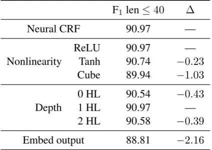
Table 1 shows results on section 22 (the develop-ment set) of the English Penn Treebank (Marcus et al., 1993), computed usingevalb. Full test re-sults and comparisons to other systems are shown in Table 4. We compare variants of our system along two axes: whether they use standard linear sparse features, nonlinear dense features from the neural net, or both, and whether any word repre-sentations (vectors or clusters) are used.
Sparse vs. neural The neural CRF (line (d) in Table 1) on its own outperforms the sparse CRF (a, b) even when the sparse CRF has a more heav-ily annotated grammar. This is a surprising re-sult: the features in the sparse CRF have been carefully engineered to capture a range of linguis-tic phenomena (Hall et al., 2014), and there is no guarantee that word vectors will capture the same. For example, at the POS tagging layer, the sparse model looks at prefixes and suffixes of words, which give the model access to morphol-ogy for predicting tags of unknown words, which typically have regular inflection patterns. By con-trast, the neural model must rely on the geometry of the vector space exposing useful regularities. At the same time, the strong performance of the combination of the two systems (g) indicates that not only are both featurization approaches high-performing on their own, but that they have com-plementary strengths.
Sparse Neural V Word Reps F1len≤40 F1all
Hall et al. (2014),V = 1 90.5
a X 0 89.89 89.22
b X 1 90.82 90.13
c X 1 Brown 90.80 90.17
d X 0 Bansal 90.97 90.44
e X 0 Collobert 90.25 89.63
f X 0 PTB 89.34 88.99
g X X 0 Bansal 92.04 91.34
[image:6.595.311.523.63.213.2]h X X 0 PTB 91.39 90.91
Table 1: Results of our sparse CRF, neural CRF, and combined parsing models on section 22 of the Penn Treebank. Systems are broken down by whether local potentials come from sparse features and/or the neural network (the primary contribution of this work), their level of vertical Markovization, and what kind of word represen-tations they use. The neural CRF (d) outperforms the sparse CRF (a, b) even when a more heavily annotated grammar is used, and the combined ap-proach (g) is substantially better than either indi-vidual model. The contribution of the neural ar-chitecture cannot be replaced by Brown clusters (c), and even word representations learned just on the Penn Treebank are surprisingly effective (f, h).
However, as these embeddings are trained on a relatively small corpus (BLLIP minus the Penn Treebank), it is natural to wonder whether less-syntactic embeddings trained on a larger corpus might be more useful. This is not the case: line (e) in Table 1 shows the performance of the neu-ral CRF using the Wikipedia-trained word embed-dings of Collobert et al. (2011), which do not per-form better than the vectors of Bansal et al. (2014). To isolate the contribution of continuous word representations themselves, we also experimented with vectors trained on just the text from the train-ing set of the Penn Treebank ustrain-ing the skip-gram model with a window size of 1. While these vec-tors are somewhat lower performing on their own (f), they still provide a surprising and noticeable gain when stacked on top of sparse features (h), again suggesting that dense and sparse represen-tations have complementary strengths. This result also reinforces the notion that the utility of word vectors does not come primarily from importing information about out-of-vocabulary words (An-dreas and Klein, 2014).
Since the neural features incorporate informa-tion from unlabeled data, we should provide the
F1len≤40 ∆
Neural CRF 90.97 —
Nonlinearity ReLUTanh 90.9790.74 −—0.23
Cube 89.94 −1.03
Depth 0 HL1 HL 90.5490.97 −0—.43
2 HL 90.58 −0.39
Embed output 88.81 −2.16
Table 2: Exploration of other implementation choices in the feedforward neural network on sen-tences of length≤40from section 22 of the Penn Treebank. Rectified linear units perform better than tanh or cubic units, a network with one hid-den layer performs best, and embedding the output feature vector gives worse performance.
sparse model with similar information for a true apples-to-apples comparison. Brown clusters have been shown to be effective vehicles in the past (Koo et al., 2008; Turian et al., 2010; Bansal et al., 2014). We can incorporate Brown clusters into the baseline CRF model in an analogous way to how embedding features are used in the dense model: surface features are fired on Brown cluster iden-tities (we use prefixes of length 4 and 10) of key words. We use the Brown clusters from Koo et al. (2008), which are trained on the same data as the vectors of Bansal et al. (2014). However, Table 1 shows that these features provide no benefit to the baseline model, which suggests either that it is dif-ficult to learn reliable weights for these as sparse features or that different regularities are being cap-tured by the word embeddings.
6 Design Choices
The neural net design space is large, so we wish to analyze the particular design choices we made for this system by examining the performance of several variants of the neural net architecture used in our system. Table 2 shows development re-sults from potential alternate architectural choices, which we now discuss.
[image:6.595.75.290.73.191.2]computer vision (Krizhevsky et al., 2012).g(x) = tanh(x) is a traditional nonlinearity widely used throughout the history of neural nets (Bengio et al., 2003).g(x) =x3(cube) was found to be most successful by Chen and Manning (2014).
Table 2 compares the performance of these three nonlinearities. We see that rectified linear units perform the best, followed by tanh units, followed by cubic units.9 One drawback of tanh
as an activation function is that it is easily “satu-rated” if the input to the unit is too far away from zero, causing the backpropagation of derivatives through that unit to essentially cease; this is known to cause problems for training, requiring special purpose machinery for use in deep networks (Ioffe and Szegedy, 2015).
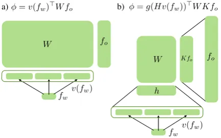
Depth Given that we are using rectified linear units, it bears asking whether or not our imple-mentation is improving substantially over linear features of the continuous input. We can use the embedding vector of an anchored spanv(fw) di-rectly as input to a basic linear CRF, as shown in Figure 4a. Table 1 shows that the purely linear ar-chitecture (0 HL) performs surprisingly well, but is still less effective than the network with one hid-den layer. This agrees with the results of Wang and Manning (2013), who noted that dense fea-tures typically benefit from nonlinear modeling. We also compare against a two-layer neural net-work, but find that this also performs worse than the one-layer architecture.
Densifying output features Overall, it appears beneficial to use dense representations of surface features; a natural question that one might ask is whether the same technique can be applied to the sparse output feature vectorfo. We can apply the approach of Srikumar and Manning (2014) and multiply the sparse output vector by a dense matrix K, giving the following scoring function (shown in Figure 4b):
φ(w, r, s;H, W, K) =g(Hv(fw(w, s)))>W Kfo(r)
where W is now nh ×noe and K is noe ×no. W Kcan be seen a low-rank approximation of the originalW at the output layer, similar to low-rank factorizations of parameter matrices used in past 9The performance of cube decreased substantially late in
learning; it peaked at around 90.52. Dropout may be useful for alleviating this type of overfitting, but in our experiments we did not find dropout to be beneficial overall.
fo W
W
h
a) b)
fo Kfo
=g(Hv(fw))>W Kfo
=v(fw)>W fo
fw v(fw) fw v(fw)
Figure 4: Two additional forms of the scoring function. a) Linear version of the dense model, equivalent to a CRF with continuous-valued input features. b) Version of the dense model where out-puts are also embedded according to a learned ma-trixK.
work (Lei et al., 2014). This approach saves us from having to learn a separate row ofW for ev-ery rule in the grammar; if rules are given similar embeddings, then they will behave similarly ac-cording to the model.
We experimented with noe = 20 and show the results in Table 2. Unfortunately, this approach does not seem to work well for parsing. Learn-ing the output representation was empirically very unstable, and it also required careful initialization. We tried Gaussian initialization (as in the rest of our model) and initializing the model by clustering rules either randomly or according to their parent symbol. The latter is what is shown in the table, and gave substantially better performance. We hy-pothesize that blurring distinctions between output classes may harm the model’s ability to differenti-ate between closely-reldifferenti-ated symbols, which is re-quired for good parsing performance. Using pre-trained rule embeddings at this layer might also improve performance of this method.
7 Test Results
We evaluate our system under two conditions: first, on the English Penn Treebank, and second, on the nine languages used in the SPMRL 2013 and 2014 shared tasks.
7.1 Penn Treebank
Arabic Basque French German Hebrew Hungarian Korean Polish Swedish Avg Dev, all lengths
Hall et al. (2014) 78.89 83.74 79.40 83.28 88.06 87.44 81.85 91.10 75.95 83.30 This work* 80.68 84.37 80.65 85.25 89.37 89.46 82.35 92.10 77.93 84.68
Test, all lengths
Berkeley 79.19 70.50 80.38 78.30 86.96 81.62 71.42 79.23 79.18 78.53 Berkeley-Tags 78.66 74.74 79.76 78.28 85.42 85.22 78.56 86.75 80.64 80.89 Crabb´e and Seddah (2014) 77.66 85.35 79.68 77.15 86.19 87.51 79.35 91.60 82.72 83.02 Hall et al. (2014) 78.75 83.39 79.70 78.43 87.18 88.25 80.18 90.66 82.00 83.17 This work* 80.24 85.41 81.25 80.95 88.61 90.66 82.23 92.97 83.45 85.08
Reranked ensemble
[image:8.595.74.527.76.220.2]2014 Best 81.32 88.24 82.53 81.66 89.80 91.72 83.81 90.50 85.50 86.12
Table 3: Results for the nine treebanks in the SPMRL 2013/2014 Shared Tasks; all values are F-scores for sentences of all lengths using the version of evalbdistributed with the shared task. Our parser substantially outperforms the strongest single parser results on this dataset (Hall et al., 2014; Crabb´e and Seddah, 2014). Berkeley-Tags is an improved version of the Berkeley parser designed for the shared task (Seddah et al., 2013). 2014 Best is a reranked ensemble of modified Berkeley parsers and constitutes the best published numbers on this dataset (Bj¨orkelund et al., 2013; Bj¨orkelund et al., 2014).
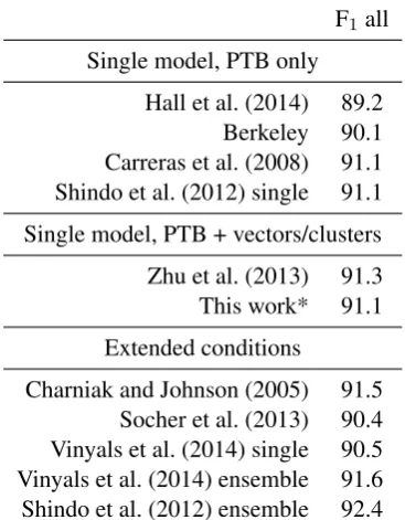
F1all Single model, PTB only
Hall et al. (2014) 89.2 Berkeley 90.1 Carreras et al. (2008) 91.1 Shindo et al. (2012) single 91.1 Single model, PTB + vectors/clusters Zhu et al. (2013) 91.3 This work* 91.1 Extended conditions
Charniak and Johnson (2005) 91.5 Socher et al. (2013) 90.4 Vinyals et al. (2014) single 90.5 Vinyals et al. (2014) ensemble 91.6 Shindo et al. (2012) ensemble 92.4
Table 4: Test results on section 23 of the Penn Treebank. We compare to several categories of parsers from the literatures. We outperform strong baselines such as the Berkeley Parser (Petrov and Klein, 2007) and the CVG Stanford parser (Socher et al., 2013) and we match the performance of so-phisticated generative (Shindo et al., 2012) and discriminative (Carreras et al., 2008) parsers.
four parsers trained only on the PTB with no aux-iliary data: the CRF parser of Hall et al. (2014), the Berkeley parser (Petrov and Klein, 2007), the discriminative parser of Carreras et al. (2008), and
the single TSG parser of Shindo et al. (2012). To our knowledge, the latter two systems are the high-est performing in this PTB-only, single parser data condition; we match their performance at 91.1 F1, though we also use word vectors computed from unlabeled data. We further compare to the shift-reduce parser of Zhu et al. (2013), which uses un-labeled data in the form of Brown clusters. Our method achieves performance close to that of their parser.
We also compare to the compositional vector grammar (CVG) parser of Socher et al. (2013) as well as the LSTM-based parser of Vinyals et al. (2014). The conditions these parsers are op-erating under are slightly different: the former is a reranker on top of the Stanford Parser (Klein and Manning, 2003) and the latter trains on much larger amounts of data parsed by a product of Berkeley parsers (Petrov, 2010). Regardless, we outperform the CVG parser as well as the single parser results from Vinyals et al. (2014).
7.2 SPMRL
[image:8.595.89.273.330.566.2](Mikolov et al., 2013).10 Here we use V = 1
in the backbone grammar, which we found to be beneficial overall. Table 3 shows that our system improves upon the performance of the parser from Hall et al. (2014) as well as the top single parser from the shared task (Crabb´e and Seddah, 2014), with robust improvements on all languages.
8 Conclusion
In this work, we presented a CRF parser that scores anchored rule productions using dense in-put features comin-puted from a feedforward neu-ral net. Because the neuneu-ral component is mod-ularized, we can easily integrate it into a pre-existing learning and inference framework based around dynamic programming of a discrete parse chart. Our combined neural and sparse model gives strong performance both on English and on other languages.
Our system is publicly available at
http://nlp.cs.berkeley.edu.
Acknowledgments
This work was partially supported by BBN un-der DARPA contract HR0011-12-C-0014, by a Facebook fellowship for the first author, and by a Google Faculty Research Award to the second author. Thanks to David Hall for assistance with the Epic parsing framework and for a preliminary implementation of the neural architecture, to Kush Rastogi for training word vectors on the SPMRL data, to Dan Jurafsky for helpful discussions, and to the anonymous reviewers for their insightful comments.
References
Jacob Andreas and Dan Klein. 2014. How much do word embeddings encode about syntax? In Pro-ceedings of the Association for Computational Lin-guistics.
Mohit Bansal, Kevin Gimpel, and Karen Livescu. 2014. Tailoring Continuous Word Representations for Dependency Parsing. InProceedings of the As-sociation for Computational Linguistics.
Yonatan Belinkov, Tao Lei, Regina Barzilay, and Amir Globerson. 2014. Exploring Compositional Archi-tectures and Word Vector Representations for Prepo-sitional Phrase Attachment. Transactions of the As-sociation for Computational Linguistics, 2:561–572.
10Training vectors with the SKIP
DEPmethod of Bansal et
al. (2014) did not substantially improve performance here.
Yoshua Bengio, R´ejean Ducharme, Pascal Vincent, and Christian Janvin. 2003. A Neural Probabilistic Lan-guage Model. Journal of Machine Learning Re-search, 3:1137–1155, March.
Anders Bj¨orkelund, Ozlem Cetinoglu, Rich´ard Farkas, Thomas Mueller, and Wolfgang Seeker. 2013. (Re)ranking Meets Morphosyntax: State-of-the-art Results from the SPMRL 2013 Shared Task. In Pro-ceedings of the Fourth Workshop on Statistical Pars-ing of Morphologically-Rich Languages.
Anders Bj¨orkelund, ¨Ozlem C¸etino˘glu, Agnieszka Fale´nska, Rich´ard Farkas, Thomas Mueller, Wolf-gang Seeker, and Zsolt Sz´ant´o. 2014. Introducing the IMS-Wrocław-Szeged-CIS entry at the SPMRL 2014 Shared Task: Reranking and Morpho-syntax meet Unlabeled Data. In Proceedings of the First Joint Workshop on Statistical Parsing of Morpho-logically Rich Languages and Syntactic Analysis of Non-Canonical Languages.
Xavier Carreras, Michael Collins, and Terry Koo. 2008. TAG, Dynamic Programming, and the Per-ceptron for Efficient, Feature-rich Parsing. In Pro-ceedings of the Conference on Computational Natu-ral Language Learning.
Eugene Charniak and Mark Johnson. 2005. Coarse-to-Fine n-Best Parsing and MaxEnt Discriminative Reranking. In Proceedings of the Association for Computational Linguistics.
Danqi Chen and Christopher D Manning. 2014. A Fast and Accurate Dependency Parser using Neural Networks. InProceedings of Empirical Methods in Natural Language Processing.
Wenliang Chen, Yue Zhang, and Min Zhang. 2014. Feature Embedding for Dependency Parsing. In Proceedings of the International Conference on Computational Linguistics.
Ronan Collobert, Jason Weston, L´eon Bottou, Michael Karlen, Koray Kavukcuoglu, and Pavel Kuksa. 2011. Natural Language Processing (Almost) from Scratch. Journal of Machine Learning Research, 12:2493–2537.
Benoit Crabb´e and Djam´e Seddah. 2014. Multilingual Discriminative Shift-Reduce Phrase Structure Pars-ing for the SPMRL 2014 Shared Task. In Proceed-ings of the First Joint Workshop on Statistical Pars-ing of Morphologically Rich Languages and Syntac-tic Analysis of Non-Canonical Languages.
John Duchi, Elad Hazan, and Yoram Singer. 2011. Adaptive Subgradient Methods for Online Learning and Stochastic Optimization. Journal of Machine Learning Research, 12:2121–2159, July.
David Hall, Greg Durrett, and Dan Klein. 2014. Less Grammar, More Features. InProceedings of the As-sociation for Computational Linguistics.
James Henderson. 2003. Inducing History Represen-tations for Broad Coverage Statistical Parsing. In Proceedings of the North American Chapter of the Association for Computational Linguistics.
Sergey Ioffe and Christian Szegedy. 2015. Batch Nor-malization: Accelerating Deep Network Training by Reducing Internal Covariate Shift. arXiv preprint, arXiv:1502.03167.
Ozan ˙Irsoy and Claire Cardie. 2014. Opinion Min-ing with Deep Recurrent Neural Networks. In Pro-ceedings of the Conference on Empirical Methods in Natural Language Processing.
Nal Kalchbrenner, Edward Grefenstette, and Phil Blun-som. 2014. A Convolutional Neural Network for Modelling Sentences. InProceedings of the Associ-ation for ComputAssoci-ational Linguistics.
Yoon Kim. 2014. Convolutional Neural Networks for Sentence Classification. InProceedings of the Con-ference on Empirical Methods in Natural Language Processing.
Dan Klein and Christopher D. Manning. 2003. Ac-curate Unlexicalized Parsing. InProceedings of the Association for Computational Linguistics.
Terry Koo, Xavier Carreras, and Michael Collins. 2008. Simple Semi-supervised Dependency Pars-ing. InProceedings of the Association for Compu-tational Linguistics.
Alex Krizhevsky, Ilya Sutskever, and Geoffrey E. Hin-ton. 2012. ImageNet Classification with Deep Con-volutional Neural Networks. InAdvances in Neural Information Processing Systems.
Phong Le and Willem Zuidema. 2014. The inside-outside recursive neural network model for depen-dency parsing. InProceedings of the Conference on Empirical Methods in Natural Language Process-ing.
Tao Lei, Yu Xin, Yuan Zhang, Regina Barzilay, and Tommi Jaakkola. 2014. Low-Rank Tensors for Scoring Dependency Structures. InProceedings of the Association for Computational Linguistics. Omer Levy and Yoav Goldberg. 2014.
Dependency-Based Word Embeddings. InProceedings of the As-sociation for Computational Linguistics.
Mitchell P. Marcus, Beatrice Santorini, and Mary Ann Marcinkiewicz. 1993. Building a Large Annotated Corpus of English: The Penn Treebank. Computa-tional Linguistics, 19(2).
Tomas Mikolov, Kai Chen, Greg Corrado, and Jeffrey Dean. 2013. Efficient Estimation of Word Repre-sentations in Vector Space. In Proceedings of the International Conference on Learning Representa-tions.
Slav Petrov and Dan Klein. 2007. Improved Infer-ence for Unlexicalized Parsing. InProceedings of the North American Chapter of the Association for Computational Linguistics.
Slav Petrov and Dan Klein. 2008. Sparse Multi-Scale Grammars for Discriminative Latent Variable Pars-ing. InProceedings of the Conference on Empirical Methods in Natural Language Processing.
Slav Petrov. 2010. Products of Random Latent Vari-able Grammars. InProceedings of the North Amer-ican Chapter of the Association for Computational Linguistics.
Djam´e Seddah, Reut Tsarfaty, Sandra K¨ubler, Marie Candito, Jinho D. Choi, Rich´ard Farkas, Jen-nifer Foster, Iakes Goenaga, Koldo Gojenola Gal-letebeitia, Yoav Goldberg, Spence Green, Nizar Habash, Marco Kuhlmann, Wolfgang Maier, Joakim Nivre, Adam Przepi´orkowski, Ryan Roth, Wolf-gang Seeker, Yannick Versley, Veronika Vincze, Marcin Woli´nski, and Alina Wr´oblewska. 2013. Overview of the SPMRL 2013 Shared Task: A Cross-Framework Evaluation of Parsing Morpho-logically Rich Languages. In Proceedings of the Fourth Workshop on Statistical Parsing of Morphologically-Rich Languages.
Djam´e Seddah, Sandra K¨ubler, and Reut Tsarfaty. 2014. Introducing the SPMRL 2014 Shared Task on Parsing Morphologically-rich Languages. In Pro-ceedings of the First Joint Workshop on Statisti-cal Parsing of MorphologiStatisti-cally Rich Languages and Syntactic Analysis of Non-Canonical Languages. Hiroyuki Shindo, Yusuke Miyao, Akinori Fujino, and
Masaaki Nagata. 2012. Bayesian Symbol-refined Tree Substitution Grammars for Syntactic Parsing. InProceedings of the Association for Computational Linguistics.
Richard Socher, John Bauer, Christopher D. Manning, and Andrew Y. Ng. 2013. Parsing With Composi-tional Vector Grammars. InProceedings of the As-sociation for Computational Linguistics.
Vivek Srikumar and Christopher D Manning. 2014. Learning Distributed Representations for Structured Output Prediction. InAdvances in Neural Informa-tion Processing Systems.
Yuta Tsuboi. 2014. Neural Networks Leverage Corpus-wide Information for Part-of-speech Tag-ging. InProceedings of the Conference on Empir-ical Methods in Natural Language Processing. Joseph Turian, Lev Ratinov, and Yoshua Bengio.
2010. Word Representations: A Simple and General Method for Semi-supervised Learning. In Proceed-ings of the Association for Computational Linguis-tics.
Mengqiu Wang and Christopher D. Manning. 2013. Effect of Non-linear Deep Architecture in Sequence Labeling. InProceedings of the International Joint Conference on Natural Language Processing. Matthew D. Zeiler. 2012. ADADELTA: An Adaptive
Learning Rate Method. CoRR, abs/1212.5701. Muhua Zhu, Yue Zhang, Wenliang Chen, Min Zhang,