1706
Unsupervised Discovery of Gendered Language
through Latent-Variable Modeling
Alexander Hoyle@ Lawrence Wolf-SonkinS Hanna WallachZ Isabelle AugensteinP Ryan CotterellH
@University College London, London, UK
SDepartment of Computer Science, Johns Hopkins University, Baltimore, USA ZMicrosoft Research, New York City, USA
HDepartment of Computer Science and Technology, University of Cambridge, Cambridge, UK
PDepartment of Computer Science, University of Copenhagen, Copenhagen, Denmark
[email protected], [email protected] [email protected], [email protected], [email protected]
Abstract
Studying the ways in which language is gen-dered has long been an area of interest in so-ciolinguistics. Studies have explored, for ex-ample, the speech of male and female charac-ters in film and the language used to describe male and female politicians. In this paper, we aim not to merely study this phenomenon qual-itatively, but instead to quantify the degree to which the language used to describe men and women is different and, moreover, different in a positive or negative way. To that end, we in-troduce a generative latent-variable model that jointly represents adjective (or verb) choice, with its sentiment, given the natural gender of a head (or dependent) noun. We find that there are significant differences between de-scriptions of male and female nouns and that these differences align with common gender stereotypes: Positive adjectives used to de-scribe women are more often related to their bodies than adjectives used to describe men.
1 Introduction
Word choice is strongly influenced by gender— both that of the speaker and that of the referent (Lakoff, 1973). Even within 24 hours of birth, parents describe their daughters asbeautiful,pretty, and cute far more often than their sons (Rubin et al.,1974). To date, much of the research in soci-olinguistics on gendered language has focused on laboratory studies and smaller corpora (McKee and Sherriffs,1957;Williams and Bennett,1975;Baker, 2005); however, more recent work has begun to fo-cus on larger-scale datasets (Pearce,2008; Caldas-Coulthard and Moon,2010;Baker,2014;Norberg, 2016). These studies compare the adjectives (or
beautiful lovely
chaste
gorgeous
fertile beauteous
sexy classy exquisite
vivacious
vibrant
battered
untreated barren
shrewish sheltered
heartbroken
unmarried
undernourished underweight
uncomplaining
nagging
just
sound
righteous
rational
peaceable
prodigious
brave
paramount
reliable
sinless
honorable
unsuitable unreliable
lawless
inseparable
brutish
idle unarmed
wounded
bigoted unjust
brutal
Male
Positive Negative Female
Positive Negative
MISCELLANEOUS
TEMPORAL
SOCIAL FEELING
SPATIAL
QUANTITY BODY
BEHAVIOR
[image:1.595.310.525.291.509.2]SUBSTANCE
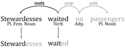
Figure 1: Adjectives, with sentiment, used to describe men and women, as represented by our model. Colors indicate the most common sense of each adjective from
Tsvetkov et al.(2014); black indicates out of lexicon. Two patterns are immediately apparent: positive adjectives describing women are often related to their bodies, while positive adjectives describing men are often related to their behavior. These patterns hold generally and the differences are significant (see§4).
verbs) that modify each noun in a particular gen-dered pair of nouns, such asboy–girl, aggregated across a given corpus. We extend this line of work by instead focusing on multiple noun pairs simulta-neously, modeling how the choice of adjective (or verb) depends on the natural gender1of the head
1A noun’s natural gender is the implied gender of its
(or dependent) noun, abstracting away the noun form. To that end, we introduce a generative latent-variable model for representing gendered language, along with sentiment, from a parsed corpus. This model allows us to quantify differences between the language used to describe men and women.
The motivation behind our approach is straight-forward: Consider the sets of adjectives (or verbs) that attach to gendered, animate nouns, such as manorwoman. Do these sets differ in ways that depend on gender? For example, we might ex-pect that the adjectiveBaltimoreanattaches toman roughly the same number of times as it attaches to woman, controlling for the frequency of man andwoman.2 But this is not the case for all adjec-tives. The adjectivepregnant, for example, almost always describes women, modulo the rare times that men are described as being pregnant with, say, emotion. Arguably, the gendered use ofpregnant is benign—it is not due to cultural bias that women are more often described as pregnant, but rather be-cause women bear children. However, differences in the use of other adjectives (or verbs) may be more pernicious. For example, female professors are less often described asbrilliantthan male pro-fessors (Storage et al.,2016), likely reflecting im-plicit or exim-plicit stereotypes about men and women. In this paper, we therefore aim to quantify the degree to which the language used to describe men and women is different and, moreover, different in a positive or negative way. Concretely, we focus on three sociolinguistic research questions about the influence of gender on adjective and verb choice:
Q1 What are thequalitativedifferences between the language used to describe men and women? For example, what, if any, are the patterns revealed by our model? Does the out-put from our model correlate with previous human judgments of gender stereotypes?
Q2 What are the quantitative differences be-tween the language used to describe men and women? For example, are adjectives used to describe women more often related to their bodies than adjectives used to describe men? Can we quantify such patterns using existing semantic resources (Tsvetkov et al.,2014)?
gender from grammatical gender because the latter does not necessarily convey anything meaningful about the referent.
2Men are written about more often than women. Indeed,
the corpus we use exhibits this trend, as shown in Tab.1.
Female Male
other 2.2 other 6.8
daughter 1.4 husband 1.8
lady 2.4 king 2.1
wife 3.3 son 2.9
mother 4.2 father 4.2
girl 5.1 boy 5.1
woman 11.5 man 39.9
[image:2.595.340.493.62.169.2]Total 30.2 62.7
Table 1: Counts, in millions, of male and female nouns present in the corpus ofGoldberg and Orwant(2013).
Q3 Does the overall sentiment of the language used to describe men and women differ?
To answer these questions, we introduce a gen-erative latent-variable model that jointly represents adjective (or verb) choice, with its sentiment, given the natural gender of a head (or dependent) noun. We use a form of posterior regularization to guide inference of the latent variables (Ganchev et al., 2010). We then use this model to study the syntac-ticn-gram corpus of (Goldberg and Orwant,2013). To answer Q1, we conduct an analysis that re-veals differences between descriptions of male and female nouns that align with common gen-der stereotypes captured by previous human judge-ments. When using our model to answer Q2, we find that adjectives used to describe women are more often related to their bodies (significant under a permutation test withp <0.03) than adjectives used to describe men (see Fig. 1 for examples). This finding accords with previous research ( Nor-berg,2016). Finally, in answer to Q3, we find no significant difference in the overall sentiment of the language used to describe men and women.
2 What Makes this Study Different?
As explained in the previous section, many soci-olinguistics researchers have undertaken corpus-based studies of gendered language. In this section, we therefore differentiate our approach from these studies and from recent NLP research on gender bi-ases in word embeddings and co-reference systems.
adjectives and verbs that attach to gendered, ani-mate nouns, we are able to more precisely quantify the degree to which the language used to describe men and women is different. To date, much of the corpus-based sociolinguistics research on gen-dered language has focused on differences between the adjectives (or verbs) that modify each noun in a particular gendered pair of nouns, such asboy– girlorman–woman(e.g.,Pearce(2008); Caldas-Coulthard and Moon(2010);Norberg(2016)). To assess the differences, researchers typically report top collocates3for one word in the pair, exclusive of collocates for the other. This approach has the effect of restricting both the amount of available data and the claims that can be made regarding gen-dered nouns more broadly. In contrast, we focus on multiple noun pairs (including plural forms) simul-taneously, modeling how the choice of adjective (or verb) depends on the natural gender of the head (or dependent) noun, abstracting away the noun form. As a result, we are able to make broader claims.
The corpus of Goldberg and Orwant (2013).
To extract the adjectives and verbs that attach to gendered, animate nouns, we use the corpus of Goldberg and Orwant (2013), who ran a then-state-of-the-art dependency parser on 3.5 million digitalized books. We believe that the size of this corpus (11 billion words) makes our study the largest collocational study of its kind. Previous studies have used corpora of under one billion words, such as the British National Corpus (100 million words) (Pearce, 2008), the New Model Corpus (100 million words) (Norberg,2016), and the Bank of English Corpus (450 million words) (Moon, Rosamund,2014). By default, the corpus ofGoldberg and Orwant (2013) is broken down by year, but we aggregate the data across years to obtain roughly 37 million noun–adjectives pairs, 41 millionNSUBJ–verb pairs, and 14 million
DOBJ–verb pairs. We additionally lemmatize each word. For example, the nounstewardesses is lemmatized to a set of lexical features consisting of the genderless lemmaSTEWARD and the mor-phological features+FEMand+PL. This parsing and lemmatization process is illustrated in Fig.2.
Quantitative evaluation. Our study is also quan-titative in nature: we test concrete hypotheses about differences between the language used to describe men and women. For example, we test whether
[image:3.595.306.527.62.147.2]3Typically ranked by the log of the Dice coefficient.
Figure 2: An example sentence with its labeled depen-dency parse (top) and lemmatized words (bottom).
women are more often described using adjectives related to their bodies and emotions. This quantita-tive focus differentiates our approach from previous corpus-based sociolinguistics research on gendered language. Indeed, in the introduction to a special issue on corpus methods in the journalGender and Language, Baker(2013) writes, “while the term corpus and its plural corpora are reasonably popu-lar within Gender and Language (occurring in al-most 40% of articles from issues 1-6), authors have mainly used the term as a synonym for ‘data set’ and have tended to carry out their analysis by hand and eye methods alone.” Moreover, in a related paper on extracting gendered language from word embeddings,Garg et al.(2018) lament that “due to the relative lack of systematic quantification of stereotypes in the literature [... they] cannot directly validate [their] results.” For an overview of quan-titative evaluation, we recommendBaker(2014).
Speaker versus referent. Many data-driven studies of gender and language focus on what speakers of different genders say rather than differences between descriptions of men and women. This is an easier task—the only annotation required is the gender of the speaker. For example, Ott(2016) used a topic model to study how word choice in tweets is influenced by the gender of the tweeter;Schofield and Mehr(2016) modeled gen-der in film dialog; and, in the realm of social media analysis,Bamman et al.(2014) discussed stylistic choices that enable classifiers to distinguish between tweets written by men versus women.
of gendered words, such as she–he, to mitigate unwanted gender biases in word embeddings. Al-though it is possible to rank the adjectives (or verbs) most aligned with the embedding subspace defined by a pair of gendered words, there are no guaran-tees that the resulting adjectives (or verbs) were specifically used to describe men or women in the dataset from which the embeddings were learned. In contrast, we use syntactic collocations to ex-plicitly represent gendered relationships between individual words. As a result, we are able make definitive claims about these relationships, thereby enabling us to answer sociolinguistic research ques-tions. Indeed, it is this sociolinguistic focus that differentiates our approach from this line of work.
3 Modeling Gendered Language
As explained in§1, our aim is quantify the degree to which the language used to describe men and women is different and, moreover, different in a positive or negative way. To do this, we therefore introduce a generative latent-variable model that jointly represents adjective (or verb) choice, with its sentiment, given the natural gender of a head (or dependent) noun. This model, which is based on the sparse additive generative model (SAGE; Eisen-stein et al.,2011),4enables us to extract ranked lists of adjectives (or verbs) that are used, with particu-lar sentiments, to describe male or female nouns.
We defineGto be the set of gendered, animate nouns in our corpus and n ∈ G to be one such noun. We represent n via a multi-hot vector
fn ∈ {0,1}T of its lexical features—i.e., its
genderless lemma, its gender (male or female), and its number (singular or plural). In other words, fn always has exactly three non-zero
entries; for example, the only non-zero entries of
fstewardessesare those corresponding toSTEWARD,
+FEM, and +PL. We define V to be the set of adjectives (or verbs) in our corpus and ν ∈ V
to be one such adjective (or verb). To simplify exposition, we refer to each adjective (or verb) that attaches to nounnas aneighborofn. Finally, we defineS = {POS,NEG,NEU}to be a set of three sentiments ands∈ S to be one such sentiment.
Drawing inspiration from SAGE, our model jointly represents nouns, neighbors, and (latent)
4SAGE is a flexible alternative to latent Dirichlet allocation
(LDA;Blei et al.,2003)—the most widely used statistical topic model. Our study could also have been conducted using LDA; drawing on SAGE was primarily a matter of personal taste.
n s
ν
Figure 3: Graphical model depicting our model’s repre-sentation of nouns, neighbors, and (latent) sentiments.
sentiments as depicted in Fig.3. Specifically,
p(ν, n, s) =p(ν|s, n)p(s|n)p(n). (1)
The first factor in eq. (1) is defined as
p(ν|s, n)∝exp{mν +fn>η(ν, s)}, (2)
wherem∈R|V|is a background distribution and η(ν, s)∈RT is a neighbor- and sentiment-specific
deviation. The second factor in eq. (1) is defined as
p(s|n)∝exp (ωns), (3)
whereωn
s ∈R, while the third factor is defined as
p(n)∝exp (ξn), (4)
whereξn∈R. We can then extract lists of
neigh-bors that are used, with particular sentiments, to describe male and female nouns, ranked by scores that are a function of their deviations. For example, the score for neighborνwhen used, with positive sentiment, to describe a male noun is defined as
τMASC-POS(ν)∝exp{g >
MASCη(ν,POS)}, (5)
wheregMASC ∈ {0,1}T is a vector where only the
entry that corresponds to+MASCis non-zero. Because our corpus does not contain explicit sentiment information, we marginalize outs:
p(ν, n) =X s∈S
p(ν|s, n)p(s|n)p(n). (6)
This yields the following objective function:
X
n∈G
X
ν∈V ˆ
p(ν, n) log (p(ν, n)), (7)
wherepˆ(ν, n)∝#(ν, n)is the empirical probabil-ity of neighborνand nounnin our corpus.
about the sentiment of neighborν, we regularize p(s|ν), as defined by our model, to be close (in the sense of KL-divergence) toq(s|ν). Specifically, we construct the following posterior regularizer:
Rpost
=KL(q(s|ν)||p(s|ν)) (8)
=−X
s∈S
q(s|ν) log (p(s|ν)) +H(q), (9)
whereH(q)is constant andp(s|ν)is defined as
p(s|ν) =X n∈G
p(s, n|ν) (10)
=X
n∈G
p(ν|n, s)p(s|n)p(n)
p(ν) . (11)
We use the combined sentiment lexicon ofHoyle et al.(2019) as q(s|ν). This lexicon represents each word’s sentiment as a three-dimensional Dirichlet distribution, thereby accounting for the relative confidence in the strength of each senti-ment and, in turn, accommodating polysemous and rare words. By using the lexicon as external infor-mation in our posterior regularizer, we can control the extent to which it influences the latent variables.
We add the regularizer in eq. (8) to the objective function in eq. (7), using a multiplierβto control the strength of the posterior regularization. We also impose anL1-regularizerα· ||η||1 to induce sparsity. The complete objective function is then
X
n∈G
X
ν∈V ˆ
p(ν, n) log (p(ν, n))
+α· ||η||1+β·Rpost. (12)
We optimize eq. (12) with respect to η(·,·), ω, andξusing the Adam optimizer (Kingma and Ba, 2015) with α and β set as described in §4. To ensure that the parameters are interpretable (e.g., to avoid a negativeη(PREGNANT,NEG)canceling out a positiveη(PREGNANT,POS))), we also con-strainη(·,·)to be non-negative, although without this constraint, our results are largely the same.
Relationship to pointwise mutual information.
Our model also recovers pointwise mutual infor-mation (PMI), which has been used previously to identify gendered language (Rudinger et al.,2017).
Proposition 1. Consider the following restricted version of our model. Letfg ∈ {0,1}2 be a
one-hot vector that represents only the gender of a noun
n. We writeginstead ofn, equivalence-classing all nouns as eitherMASCorFEM. Letη?(·) :V →R2
be the maximum-likelihood estimate for the special case of our model without (latent) sentiments:
p(ν |g)∝exp(mν+fg>η?(ν)). (13)
Then, we have
τg(ν)∝exp(PMI(ν, g)). (14)
Proof. See App.B.
Proposition1 says that if we use a limited set of lexical features (i.e., only gender) and estimate our model without any regularization or latent sentiments, then ranking the neighbors by τg(ν)
(i.e., by their deviations from the background distribution) is equivalent to ranking them by their PMI. This proposition therefore provides insight into how our model builds on PMI. Specifically, in contrast to PMI, 1) our model can consider lexical features other than gender, 2) our model is regularized to avoid the pitfalls of maximum-likelihood estimation, and 3) our model cleanly incorporates latent sentiments, relying on posterior regularization to ensure that the p(s|ν) is close to the sentiment lexicon ofHoyle et al.(2019).
4 Experiments, Results, and Discussion
We use our model to study the corpus ofGoldberg and Orwant(2013) by running it separately on the noun–adjectives pairs, theNSUBJ–verb pairs, and theDOBJ–verb pairs. We provide a full list of the lemmatized, gendered, animate nouns in App.A. We use α ∈ {0,10−5,10−4,0.001,0.01} and β ∈ {10−5,10−4,0.001,0.01,0.1,1,10,100}; when we report results below, we use parameter val-ues averaged over these hyperparameter settings.
4.1 Q1:QualitativeDifferences
Our first research question concerns the qualitative differences between the language used to describe men and women. To answer this question, we use our model to extract ranked lists of neighbors that are used, with particular sentiments, to describe male and female nouns. As explained in§3, we rank the neighbors by their deviations from the background distribution (see, for example, eq. (5)).
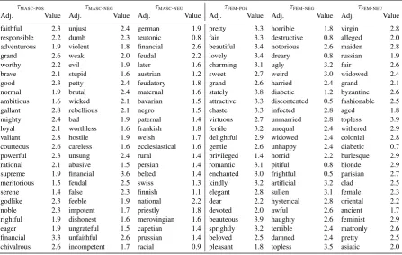
τMASC-POS τMASC-NEG τMASC-NEU τFEM-POS τFEM-NEG τFEM-NEU
Adj. Value Adj. Value Adj. Value Adj. Value Adj. Value Adj. Value
faithful 2.3 unjust 2.4 german 1.9 pretty 3.3 horrible 1.8 virgin 2.8
responsible 2.2 dumb 2.3 teutonic 0.8 fair 3.3 destructive 0.8 alleged 2.0
adventurous 1.9 violent 1.8 financial 2.6 beautiful 3.4 notorious 2.6 maiden 2.8
grand 2.6 weak 2.0 feudal 2.2 lovely 3.4 dreary 0.8 russian 1.9
worthy 2.2 evil 1.9 later 1.6 charming 3.1 ugly 3.2 fair 2.6
brave 2.1 stupid 1.6 austrian 1.2 sweet 2.7 weird 3.0 widowed 2.4
good 2.3 petty 2.4 feudatory 1.8 grand 2.6 harried 2.4 grand 2.1
normal 1.9 brutal 2.4 maternal 1.6 stately 3.8 diabetic 1.2 byzantine 2.6
ambitious 1.6 wicked 2.1 bavarian 1.5 attractive 3.3 discontented 0.5 fashionable 2.5
gallant 2.8 rebellious 2.1 negro 1.5 chaste 3.3 infected 2.8 aged 1.8
mighty 2.4 bad 1.9 paternal 1.4 virtuous 2.7 unmarried 2.8 topless 3.9
loyal 2.1 worthless 1.6 frankish 1.8 fertile 3.2 unequal 2.4 withered 2.9
valiant 2.8 hostile 1.9 welsh 1.7 delightful 2.9 widowed 2.4 colonial 2.8
courteous 2.6 careless 1.6 ecclesiastical 1.6 gentle 2.6 unhappy 2.4 diabetic 0.7
powerful 2.3 unsung 2.4 rural 1.4 privileged 1.4 horrid 2.2 burlesque 2.9
rational 2.1 abusive 1.5 persian 1.4 romantic 3.1 pitiful 0.8 blonde 2.9
supreme 1.9 financial 3.6 belted 1.4 enchanted 3.0 frightful 0.5 parisian 2.7
meritorious 1.5 feudal 2.5 swiss 1.3 kindly 3.2 artificial 3.2 clad 2.5
serene 1.4 false 2.3 finnish 1.1 elegant 2.8 sullen 3.1 female 2.3
godlike 2.3 feeble 1.9 national 2.2 dear 2.2 hysterical 2.8 oriental 2.2
noble 2.3 impotent 1.7 priestly 1.8 devoted 2.0 awful 2.6 ancient 1.7
rightful 1.9 dishonest 1.6 merovingian 1.6 beauteous 3.9 haughty 2.6 feminist 2.9
eager 1.9 ungrateful 1.5 capetian 1.4 sprightly 3.2 terrible 2.4 matronly 2.6
financial 3.3 unfaithful 2.6 prussian 1.4 beloved 2.5 damned 2.4 pretty 2.5
[image:6.595.76.524.63.347.2]chivalrous 2.6 incompetent 1.7 racial 0.9 pleasant 1.8 topless 3.5 asiatic 2.0
Table 2: For each sentiment, we provide the largest-deviation adjectives used to describe male and female nouns.
results are striking: it is immediately apparent that positive adjectives describing women are often re-lated to their appearance (e.g.,beautiful,fair, and pretty). Sociolinguistic studies of other corpora, such as British newspapers (Caldas-Coulthard and Moon,2010), have also revealed this pattern. Ad-jectives relating to fertility, such asfertileand bar-ren, are also more prevalent for women. We pro-vide similar tables for verbs in App.D. Negative verbs describing men are often related to violence (e.g.,murder,fight,kill, andthreaten). Meanwhile, women are almost always the object ofrape, which aligns with our knowledge of the world and sup-ports the collocation of rape and girl found by Baker(2014). Broadly speaking, positive verbs describing men tend to connote virtuosity (e.g., gal-lantandinspire), while those describing women ap-pear more trivial (e.g.,sprightly,giggle, andkiss).
Correlation with human judgments. To deter-mine whether the output from our model accords with previous human judgements of gender stereo-types, we use the corpus of Williams and Ben-nett (1975), which consists of 63 adjectives an-notated with (binary) gender stereotypes. We mea-sure Spearman’sρbetween these annotations and the probabilities output by our model. We find a relatively strong positive correlation ofρ = 0.59
(p <10−6), which indicates that the output from our model aligns with common gender stereotypes captured by previous human judgements. We also measure the correlation between continuous annota-tions of 300 adjectives from two follow-up studies (Williams and Best, 1990,1977)5 and the proba-bilities output by our model. Here, the correlation isρ= 0.33(p <10−8), and the binarized annota-tions agree with the output from our model for64%
of terms. We note that some of the disagreement is due to reporting bias (Gordon and Van Durme, 2013) in our corpus. For example, only men are described in our corpus as effeminate, although humans judge it to be a highly feminine adjective.
4.2 Q2:Quantitativedifferences
Our second research question concerns the quan-titative differences between the language used to describe men and women. To answer this question, we use two existing semantic resources—one for adjectives (Tsvetkov et al.,2014) and one for verbs (Miller et al., 1993)—to quantify the patterns revealed by our model. Again, we use our model to extract ranked lists of neighbors that are used, with particular sentiments, to describe male and female nouns. We consider only the 200 largest-deviation
5The studies consider the same set of words 20 years apart;
POS–BOD Y
POS–MISC NEG–MOTIONNEG–SP
ATIAL
NEU–BEHA VIOR
NEU–BOD Y
NEU–FEELINGNEU–SOCIAL
0.00 0.05 0.10 0.15 0.20 0.25
[image:7.595.76.287.64.235.2]Masc Fem
Figure 4: The frequency with which the 200 largest-deviation adjectives for each sentiment and gender cor-respond to each sense fromTsvetkov et al.(2014).
neighbors for each sentiment and gender. This restriction allows us to perform an unpaired permutation test (Good, 2004) to determine whether there are significant differences between the language used to describe men and women.
Adjective evaluation. Women are supposedly more often described using adjectives related to their bodies and emotions. For example,de Beau-voir(1953) writes that “from girlhood, women are socialized to live and experience their bodies as ob-jects for another’s gaze...” Although studies of rea-sonably large corpora have found evidence to sup-port this supposition (Norberg,2016), none have done so at scale with statistical significance test-ing. We use the semantic resource of Tsvetkov et al.(2014), which categorizes adjectives into thir-teen senses: BEHAVIOR,BODY,FEELING,MIND, etc. Specifically, each adjective has a distribution over senses, capturing how often the adjective cor-responds to each sense. We analyze the largest-deviation adjectives for each sentiment and gender by computing the frequency with which these adjec-tives correspond to each sense. We depict these fre-quencies in Fig.4. Specifically, we provide frequen-cies for the senses where, after Bonferroni correc-tion, the differences between men and women are significant. We find that adjectives used to describe women are indeed more often related to their bodies and emotions than adjectives used to describe men.
Verb evaluation. To evalaute verbs senses, we take the same approach as for adjectives. We use the semantic resource ofMiller et al.(1993), which
POS–CONT ACT
NEG–BOD Y
NEG–COMM.
0.00 0.05 0.10 0.15 0.20 0.25
Masc Fem
Figure 5: The frequency with which the 200 largest-deviation verbs for each sentiment and gender corre-spond to each sense fromMiller et al.(1993). These re-sults are only for theNSUBJ–verb pairs; there are no sta-tistically significant differences forDOBJ–verb pairs.
ADJ NSUBJ DOBJ
MSC FEM MSC FEM MSC FEM
POS 0.34 0.38 0.37 0.36 0.37 0.36
NEG 0.30 0.31 0.33 0.34 0.34 0.35
[image:7.595.308.525.64.236.2]NEU 0.36 0.31 0.30 0.30 0.30 0.29
Table 3: The frequency with which the 200 largest-deviation neighbors for each gender correspond to each sentiment, obtained using a simplified version of our model and the lexicon ofHoyle et al.(2019). Sig-nificant differences (p <0.05/3under an unpaired per-mutation test with Bonferroni correction) are in bold.
categorizes verbs into fifteen senses. Each verb has a distribution over senses, capturing how often the verb corresponds to each sense. We consider two cases: the NSUBJ–verb pairs and the DOBJ–verb pairs. Overall, there are fewer significant differ-ences for verbs than there are for adjectives. There are no statistically significant differences for the
DOBJ–verb pairs. We depict the results for the
NSUBJ–verb pairs in Fig. 5. We find that verbs used to describe women are more often related to their bodies than verbs used to describe men.
4.3 Q3: Differences insentiment
neighbors for each gender by computing the fre-quency with which each neighbor corresponds to each sentiment. We report these frequencies in Tab.3. We find that there is only one significant dif-ference: adjectives used to describe men are more often neutral than those used to describe women.
5 Conclusion and Limitations
We presented an experimental framework for quan-titatively studying the ways in which the language used to describe men and women is different and, moreover, different in a positive or negative way. We introduced a generative latent-variable model that jointly represents adjective (or verb) choice, with its sentiment, given the natural gender of a head (or dependent) noun. Via our experiments, we found evidence in support of common gender stereotypes. For example, positive adjectives used to describe women are more often related to their bodies than adjectives used to describe men. Our study has a few limitations that we wish to highlight. First, we ignore demographics (e.g., age, gender, location) of the speaker, even though such demographics are likely influence word choice. Second, we ignore genre (e.g., news, romance) of the text, even though genre is also likely to influ-ence the language used to describe men and women. In addition, depictions of men and women have certainly changed over the period covered by our corpus; indeed,Underwood et al.(2018) found ev-idence of such a change for fictional characters. In future work, we intend to conduct a diachronic anal-ysis in English using the same corpus, in addition to a cross-linguistic study of gendered language.
Acknowledgments
We would like to thank the three anonymous ACL 2019 reviewers for their comments on the submit-ted version, as well as the anonymous reviewers of a previous submission. We would also like to thank Adina Williams and Eleanor Chodroff for their comments on versions of the manuscript. The last author would like to acknowledge a Facebook fellowship.
References
Paul Baker. 2005.Public discourses of gay men. Rout-ledge.
Paul Baker. 2013. Introduction: Virtual special issue of
gender and language on corpus approaches.Gender and Language, 1(1).
Paul Baker. 2014. Using corpora to analyze gender. A&C Black.
David Bamman, Jacob Eisenstein, and Tyler Schnoe-belen. 2014. Gender identity and lexical varia-tion in social media. Journal of Sociolinguistics, 18(2):135–160.
Simone de Beauvoir. 1953. The second sex.
David M. Blei, Andrew Y. Ng, and Michael I. Jordan. 2003. Latent Dirichlet allocation. Journal of Ma-chine Learning Research, 3(Jan):993–1022.
Tolga Bolukbasi, Kai-Wei Chang, James Y. Zou, Venkatesh Saligrama, and Adam T. Kalai. 2016. Man is to computer programmer as woman is to homemaker? Debiasing word embeddings. In Ad-vances in Neural Information Processing Systems, pages 4349–4357.
Carmen Rosa Caldas-Coulthard and Rosamund Moon. 2010.‘Curvy, hunky, kinky’: Using corpora as tools for critical analysis.Discourse & Society, 21(2):99– 133.
Jacob Eisenstein, Amr Ahmed, and Eric P Xing. 2011. Sparse Additive Generative Models of Text. page 8.
Kuzman Ganchev, Jennifer Gillenwater, Ben Taskar, et al. 2010. Posterior regularization for structured latent variable models. Journal of Machine Learn-ing Research, 11(Jul):2001–2049.
Nikhil Garg, Londa Schiebinger, Dan Jurafsky, and James Zou. 2018. Word embeddings quantify 100 years of gender and ethnic stereotypes. Pro-ceedings of the National Academy of Sciences, 115(16):E3635–E3644.
Yoav Goldberg and Jon Orwant. 2013. A dataset of syntactic-ngrams over time from a very large corpus of English books. In Second Joint Conference on Lexical and Computational Semantics (*SEM), Vol-ume 1: Proceedings of the Main Conference and the Shared Task: Semantic Textual Similarity, pages 241–247, Atlanta, Georgia, USA. Association for Computational Linguistics.
Phillip I. Good. 2004. Permutation, parametric, and bootstrap tests of hypotheses.
Jonathan Gordon and Benjamin Van Durme. 2013.
Reporting Bias and Knowledge Acquisition. In
Proceedings of the 2013 Workshop on Automated Knowledge Base Construction, AKBC ’13, pages 25–30, New York, NY, USA. ACM.
the Association for Computational Linguistics: Hu-man Language Technologies, Volume 2 (Short Pa-pers). Association for Computational Linguistics.
Diederik P. Kingma and Jimmy Ba. 2015. Adam: A method for stochastic optimization. InInternational Conference on Learning Representations (ICLR).
Robin Lakoff. 1973. Language and woman’s place.
Language in Society, 2(1):45–79.
John P. McKee and Alex C. Sherriffs. 1957. The differ-ential evaluation of males and females. Journal of Personality, 25(3):356–371.
George A. Miller, Claudia Leacock, Randee Tengi, and Ross T. Bunker. 1993. A semantic concordance. In
Proceedings of the workshop on Human Language Technology (HLT), pages 303–308. Association for Computational Linguistics.
Moon, Rosamund. 2014. From gorgeous to grumpy: Adjectives, age, and gender. Gender and Language, 8(1):5–41.
Cathrine Norberg. 2016. Naughty Boys and Sexy Girls: The Representation of Young Individuals in a Web-Based Corpus of English. Journal of English Lin-guistics, 44(4):291–317.
Cathy O’Neil. 2016. Weapons of math destruction: How big data increases inequality and threatens democracy. Broadway Books.
Margaret Ott. 2016. Tweet like a girl: Corpus analysis of gendered language in social media.
Michael Pearce. 2008. Investigating the collocational behaviour of man and woman in the BNC using Sketch Engine.Corpora, 3(1):1–29.
Jeffrey Z. Rubin, Frank J. Provenzano, and Zella Luria. 1974. The eye of the beholder: Parents’ views on sex of newborns. American Journal of Orthopsychiatry, 44(4):512.
Rachel Rudinger, Chandler May, and Benjamin Van Durme. 2017. Social bias in elicited natural lan-guage inferences. In Proceedings of the First ACL Workshop on Ethics in Natural Language Process-ing, pages 74–79.
Rachel Rudinger, Aaron Steven White, and Benjamin Van Durme. 2018. Neural models of factuality. In
Proceedings of the 2018 Conference of the North American Chapter of the Association for Computa-tional Linguistics: Human Language Technologies, Volume 1 (Long Papers), pages 731–744. Associa-tion for ComputaAssocia-tional Linguistics.
Alexandra Schofield and Leo Mehr. 2016. Gender-distinguishing features in film dialogue. In Proceed-ings of the Fifth Workshop on Computational Lin-guistics for Literature, pages 32–39, San Diego, Cal-ifornia, USA. Association for Computational Lin-guistics.
Daniel Storage, Zachary Horne, Andrei Cimpian, and Sarah-Jane Leslie. 2016. The frequency of “bril-liant” and “genius” in teaching evaluations predicts the representation of women and African Americans across fields. PloS one, 11(3):e0150194.
Yulia Tsvetkov, Nathan Schneider, Dirk Hovy, Archna Bhatia, Manaal Faruqui, and Chris Dyer. 2014. Augmenting English adjective senses with super-senses. In Proceedings of the Ninth International Conference on Language Resources and Evaluation (LREC’14), Reykjavik, Iceland. European Language Resources Association (ELRA).
Ted Underwood, David Bamman, and Sabrina Lee. 2018. The transformation of gender in english-language fiction.
John E. Williams and Susan M. Bennett. 1975. The definition of sex stereotypes via the adjective check list. Sex Roles, 1(4):327–337.
John E. Williams and Deborah L. Best. 1977. Sex Stereotypes and Trait Favorability on the Adjective Check List. Educational and Psychological Mea-surement, 37(1):101–110.
John E. Williams and Deborah L. Best. 1990. Measur-ing sex stereotypes: a multination study. Newbury Park, Calif. : Sage.
Jieyu Zhao, Tianlu Wang, Mark Yatskar, Vicente Or-donez, and Kai-Wei Chang. 2017. Men also like shopping: Reducing gender bias amplification using corpus-level constraints. InProceedings of the 2017 Conference on Empirical Methods in Natural Lan-guage Processing, pages 2979–2989, Copenhagen, Denmark. Association for Computational Linguis-tics.
A List of Gendered, Animate Nouns
[image:10.595.307.528.102.397.2]Tab. 4contains the full list of gendered, animate nouns that we use. We consider each row in this table to be the inflected forms of a single lemma.
Male Female
Singular Plural Singular Plural
man men woman women
boy boys girl girls
father fathers mother mothers
son sons daughter daughters
brother brothers sister sisters
husband husbands wife wives
uncle uncles aunt aunts
nephew nephews niece nieces
emperor emperors empress empresses
king kings queen queens
prince princes princess princesses
duke dukes duchess duchesses
lord lords lady ladies
knight knights dame dames
waiter waiters waitress waitresses
actor actors actress actresses
god gods goddess goddesses
policeman policemen policewoman policewomen postman postmen postwoman postwomen
hero heros heroine heroines
wizard wizards witch witches
steward stewards stewardess stewardesses
he – she –
Table 4: Gendered, animate nouns.
B Relationship to PMI
Proposition 1. Consider the following restricted version of our model. Letfg ∈ {0,1}2 be a
one-hot vector that represents only the gender of a noun. We writeginstead ofn, equivalence-classing all nouns as eitherMASCorFEM. Letη?(·) :V →R2 be the maximum-likelihood estimate for the special case of our model without (latent) sentiments:
p(ν|g)∝exp(mν+fg>η?(ν)). (15)
Then, we have
τg(ν)∝exp(PMI(ν, g)). (16)
Proof. First, we note our model has enough param-eters to fit the empirical distribution exactly:
ˆ
p(ν |g) =p(ν |g) (17)
∝exp{mν+fg>η?(ν)}. (18)
Then, we proceed with an algebraic manipulation of the definition of pointwise mutual information:
PMI(ν, g) = log pˆ(ν, n) ˆ
p(ν) ˆp(n) (19)
= logpˆ(ν |n) ˆ
p(ν) (20)
= logp(ν |n) ˆ
p(ν) (21)
= log p(ν |n) exp{mν}
(22)
= log 1
Z
exp{mν+fg>η?(ν)} exp{mν}
(23)
= log 1
Z exp{f
>
g η?(ν)} (24)
=fg>η?(ν)−logZ. (25)
Now we have
τg(ν)∝exp{fg>η?(ν)} (26)
∝exp{fg>η?(ν)−logZ} (27)
= exp(PMI(ν, g)), (28)
which is what we wanted to show.
C Senses
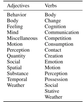
In Tab.5, we list the senses for adjectives (Tsvetkov et al.,2014) and for verbs (Miller et al.,1993).
Adjectives Verbs
Behavior Body
Body Change
Feeling Cognition
Mind Communication
Miscellaneous Competition
Motion Consumption
Perception Contact Quantity Creation
Social Emotion
Spatial Motion
Substance Perception Temporal Possession Weather Social
[image:10.595.72.290.138.439.2]Stative Weather
Table 5: Senses for adjectives and verbs.
D Additional Results
[image:10.595.344.484.469.642.2]τMASC-POS τMASC-NEG τMASC-NEU τFEM-POS τFEM-NEG τFEM-NEU
Verb Value Verb Value Verb Value Verb Value Verb Value Verb Value
succeed 1.6 fight 1.2 extend 0.7 celebrate 2.4 persecute 2.1 faint 0.7
protect 1.4 fail 1.0 found 0.8 fascinate 0.8 faint 1.0 be 1.1
favor 1.3 fear 1.0 strike 1.3 facilitate 0.7 fly 1.0 go 0.4
flourish 1.3 murder 1.5 own 1.1 marry 1.8 weep 2.3 find 0.1
prosper 1.7 shock 1.6 collect 1.1 smile 1.8 harm 2.2 fly 0.4
support 1.5 blind 1.6 set 0.8 fan 0.8 wear 2.0 fall 0.1
promise 1.5 forbid 1.5 wag 1.0 kiss 1.8 mourn 1.7 wear 0.9
welcome 1.5 kill 1.3 present 0.9 champion 2.2 gasp 1.1 leave 0.7
favour 1.2 protest 1.3 pretend 1.1 adore 2.0 fatigue 0.7 fell 0.1
clear 1.9 cheat 1.3 prostrate 1.1 dance 1.7 scold 1.8 vanish 1.3
reward 1.8 fake 0.8 want 0.9 laugh 1.6 scream 2.1 come 0.7
appeal 1.6 deprive 1.5 create 0.9 have 1.4 confess 1.7 fertilize 0.6
encourage 1.5 threaten 1.3 pay 1.1 play 1.0 get 0.5 flush 0.5
allow 1.5 frustrate 0.9 prompt 1.0 give 0.8 gossip 2.0 spin 1.6
respect 1.5 fright 0.9 brazen 1.0 like 1.8 worry 1.8 dress 1.4
comfort 1.4 temper 1.4 tarry 0.7 giggle 1.4 be 1.3 fill 0.2
treat 1.3 horrify 1.4 front 0.5 extol 0.6 fail 0.4 fee 0.2
brave 1.7 neglect 1.4 flush 0.3 compassionate 1.9 fight 0.4 extend 0.1
rescue 1.5 argue 1.3 reach 0.9 live 1.4 fake 0.3 sniff 1.6
win 1.5 denounce 1.3 escape 0.8 free 0.9 overrun 2.4 celebrate 1.1
warm 1.5 concern 1.2 gi 0.7 felicitate 0.6 hurt 1.8 clap 1.1
praise 1.4 expel 1.7 rush 0.6 mature 2.2 complain 1.7 appear 0.9
fit 1.4 dispute 1.5 duplicate 0.5 exalt 1.7 lament 1.5 gi 0.8
wish 1.4 obscure 1.4 incarnate 0.5 surpass 1.7 fertilize 0.5 have 0.5
[image:11.595.75.525.76.380.2]grant 1.3 damn 1.4 freeze 0.5 meet 1.1 feign 0.5 front 0.5
Table 6: The largest-deviation verbs used to describe male and female nouns forNSUBJ–verb pairs.
τMASC-POS τMASC-NEG τMASC-NEU τFEM-POS τFEM-NEG τFEM-NEU
Verb Value Verb Value Verb Value Verb Value Verb Value Verb Value
praise 1.7 fight 1.8 set 1.5 marry 2.3 forbid 1.3 have 1.0
thank 1.7 expel 1.8 pay 1.2 assure 3.4 shame 2.5 expose 0.8
succeed 1.7 fear 1.6 escape 0.4 escort 1.2 escort 1.3 escort 1.4
exalt 1.2 defeat 2.4 use 2.1 exclaim 1.0 exploit 0.9 pour 2.1
reward 1.8 fail 1.3 expel 0.9 play 2.7 drag 2.1 marry 1.3
commend 1.7 bribe 1.8 summon 1.7 pour 2.6 suffer 2.2 take 1.1
fit 1.4 kill 1.6 speak 1.3 create 2.0 shock 2.1 assure 1.6
glorify 2.0 deny 1.5 shop 2.6 have 1.8 fright 2.4 fertilize 1.6
honor 1.6 murder 1.7 excommunicate 1.3 fertilize 1.8 steal 2.0 ask 1.0
welcome 1.9 depose 2.3 direct 1.1 eye 0.9 insult 1.8 exclaim 0.6
gentle 1.8 summon 2.0 await 0.9 woo 3.3 fertilize 1.6 strut 2.3
inspire 1.7 order 1.9 equal 0.4 strut 3.1 violate 2.4 burn 1.7
enrich 1.7 denounce 1.7 appoint 1.7 kiss 2.6 tease 2.3 rear 1.5
uphold 1.5 deprive 1.6 animate 1.1 protect 2.1 terrify 2.1 feature 0.9
appease 1.5 mock 1.6 follow 0.7 win 2.0 persecute 2.1 visit 1.3
join 1.4 destroy 1.5 depose 1.8 excel 1.6 cry 1.8 saw 1.3
congratulate 1.3 deceive 1.7 want 1.1 treat 2.3 expose 1.3 exchange 0.8
extol 1.1 bore 1.6 reach 0.9 like 2.2 burn 2.6 shame 1.6
respect 1.7 bully 1.5 found 0.8 entertain 2.0 scare 2.0 fade 1.2
brave 1.7 enrage 1.4 exempt 0.4 espouse 1.4 frighten 1.8 signal 1.2
greet 1.6 shop 2.7 tip 1.8 feature 1.2 distract 2.3 see 1.2
restore 1.5 elect 2.2 elect 1.7 meet 2.2 weep 2.3 present 1.0
clear 1.5 compel 2.1 unmake 1.5 wish 1.9 scream 2.3 leave 0.8
excite 1.2 offend 1.5 fight 1.2 fondle 1.9 drown 2.1 espouse 1.3
flatter 0.9 scold 1.4 prevent 1.1 saw 1.8 rape 2.0 want 1.1
[image:11.595.72.527.434.729.2]