ISSN Online: 2152-7393 ISSN Print: 2152-7385
DOI: 10.4236/am.2019.102005 Feb. 15, 2019 51 Applied Mathematics
A Probabilistic Method to Determine Whether
the Speed of Light Is Constant
Motohisa Osaka
Department of Basic Science, Nippon Veterinary and Life Science University, Tokyo, Japan
Abstract
Although the formula of mass-energy equivalence was derived from the hy-pothesis that the speed of light in free space is constant, conversely, the pur-pose of this research is to show that a method of probabilistically determining whether the speed of light is constant is derived from this formula. By consi-dering the formula of mass-energy equivalence to be a function of the energy of an object moving at speed V, the probability density function (PDF) of the energy can be obtained using the inverse function of this formula, if the speed of light obeys a probability distribution. The main result is that the PDF of the energy diverges to infinity at a certain energy value regardless of the PDF of the speed of light. Thus, when the speed calculated from this value enters a certain range of the speed of light as V increases stepwise from below 299,792,458 m/s, the PDF of the energy should increase abruptly. If not, then the speed of light is constant. This is the method of probabilistically deter-mining whether the speed of light is constant. An experimental method is proposed to confirm this.
Keywords
Special Relativity, Light Speed, Mass-Energy Equivalence
1. Introduction
Albert Einstein published the theory of special relativity in 1905 [1]. The theory is on the relationship between space and time. One of its results is mass-energy equivalence: E = mc2, where E is the energy of an object when it is moving, m is
its mass while moving and c is the speed of light. This is derived from two hy-potheses. One is that the speed of light in free space is constant for all observers, regardless of their relative motion or of the motion of the light source. This hy-pothesis is generally considered verified by the Michelson-Morley experiment,
How to cite this paper: Osaka, M. (2019) A Probabilistic Method to Determine Whe- ther the Speed of Light Is Constant. Ap-plied Mathematics, 10, 51-59.
https://doi.org/10.4236/am.2019.102005
Received: January 16, 2019 Accepted: February 12, 2019 Published: February 15, 2019
Copyright © 2019 by author(s) and Scientific Research Publishing Inc. This work is licensed under the Creative Commons Attribution International License (CC BY 4.0).
DOI: 10.4236/am.2019.102005 52 Applied Mathematics which shows the differences between the speed of light in the direction of mo-tion of the earth and that in different direcmo-tions are within experimental errors
[2]. This was supported by similar experiments with higher resolutions [3] [4]. However, these experiments do not show that the speed of light in free space is constant in all inertial systems. A team at University of Glasgow reported that photon group velocity was reduced using time-correlated photon pairs and that the delay was several micrometers over a propagation distance of the order of 1 m [5]. Although they showed that adding spatial structure to an optical beam of single photons reduced the speed of light, the significance of their study was considered to be limited. The findings do not affect the formula of energy-mass equivalence because c in the formula is still regarded as the maximum speed of all objects in free space. However, the question is whether the maximum speed is constant. This study presents a probabilistic method derived from E = mc2 to
determine whether the speed of light is constant.
2. Mathematical Steps
It assumes that the speed of light obeys a probability distribution. The formula E = mc2 is also expressed as
2 0
2 , 1
m
E c
V c =
−
(1)
where m0 is the rest mass of the object, and V is its speed; V < c.
The assumptions are: 1) m0 and V are constant.
2) c obeys a probability distribution between ca and cb; ca < cb. Two probability
distributions are adopted: a uniform distribution and a triangular distribution. Then, the probability density function (PDF) of E is calculated by obtaining the inverse function of E as follows.
Step 1: Determining the inverse function of E
As 0< V/c <1, V/c is defined by sinθ (0< θ < π/2). From (1),
2 0
3 .
cos cos
m V E
θ θ
=
− (2)
Then, cosθ is represented as y:
2 . 1
V c
y =
− (3)
Representing m0V2 as P0, the following third-order equation for y is obtained
from (2):
( )
3 P0 0.f y y y
E
= − + = (4)
DOI: 10.4236/am.2019.102005 53 Applied Mathematics other words, at least one of the three roots of f(y) is between 0 and 1. As the roots of f(y) are intersections of g y
( )
=y3− =y y(
1−y)(
1+y)
and h(y) =−P0/E, all three roots are real. Two of them are between 0 and 1 and the
remain-ing root is negative. The two roots between 0 and 1 are denoted as y1 and y2; y1 ≤
y2. As 0< y < 1, the negative root is neglected. Since y1 and y2 are determined by
E, it is necessary to find out whether the inverse function of E, c ≡ h(E), is a
two-valued or single-valued function.
Step 2: Determining whether E is a two-valued or singled-valued function From (1), E has the minimum 3 32 P0 (P0 = m0V2) at 6
2 m
c ≡ V. Three
cases are examined on the basis of whether cm is between ca and cb.
Case 1: cm ≤ca
Then 6
3 a
V ≤ C . As E increases monotonically between ca and cb,
2 2
1 2
and .
1 a a 1 b
V c c V c
y < ≤ y ≤
− − (5)
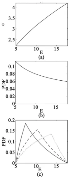
Therefore, only y2 is accepted. In this case c = h(E) is a single-valued function
[image:3.595.315.427.357.647.2](Figure 1(a)).
Figure 1. Case of cm≤ca. The object speed and limits of c are set to V = 0.5, ca = 2.2 and
DOI: 10.4236/am.2019.102005 54 Applied Mathematics Case 2: ca <cm <cb
Then 36Ca < <V 36Cb. As E is parabolic and downward convex between
ca and cb, the following relationship occurs:
2
1 22
.
1 1
a V V b
c c
y y
< < <
− − (6)
Both y1 and y2 are accepted and c = h(E) is a two-valued function (Figure 2(a)). Otherwise, the following occurs:
2 2
2 1
or .
1 a b 1
V c c V
y < < y
− − (7)
[image:4.595.306.438.269.603.2]Then c = h(E) is single-valued function (only y2 is accepted in Figure 2(a)).
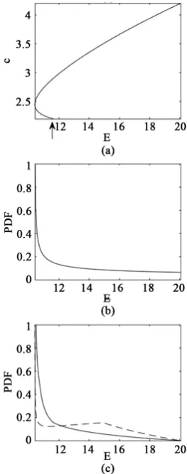
Figure 2. Case of ca<cm<cb. The object speed and limits of c are set to V = 2, ca = 2.2
and cb = 4.2. Then, cm ≈ 2.4995. (a) The inverse function of E is a two-valued function between minimum E and the value marked with an arrow and a one-valued function be-tween the marked value and maximum E; (b) Probability distribution of E when c obeys the uniform distribution; (c) Probability distribution of E for two cases: the c-value of the vertex of the triangular probability distribution of c is less than cm, (2.3 < cm) (solid line), and larger than cm, (3.7 > cm), (dashed line). In the former, the PDF of E decreases mono-tonically. In the latter, it has a vertex. If ca<cm<cb, the probability density of E is
DOI: 10.4236/am.2019.102005 55 Applied Mathematics Case 3: cm ≥cb
Then 6
3 b
V ≥ C . As E decreases monotonically between ca and cb,
12 22
and .
1 1
a V b b V
c c c
y y
≤ ≤ <
− − (8)
Therefore, only y1 is accepted. In this case c = h(E) is also a single-valued
function (Figure 3(a)).
Step 3: Calculation of PDF of E
From the PDF of c, fc(c), and the inverse function of E, c = h(E), the PDF of
the random variable E, fE(E), can be obtained as
( )
( )
d( )
d
E c
f E f h E h E
E
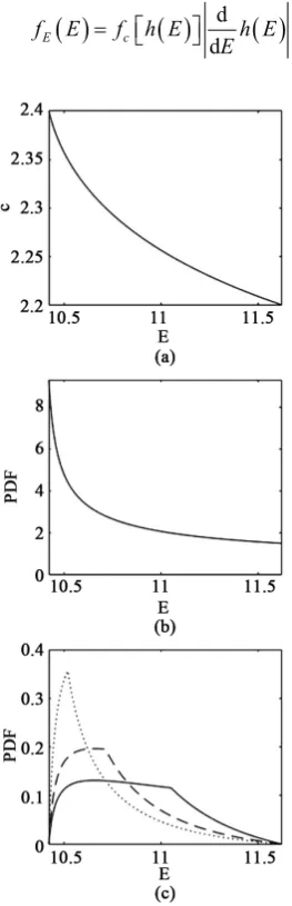
[image:5.595.309.441.234.643.2]= (9)
Figure 3. Case of cm≥cb. The object speed and limits of c are set to V = 2, ca = 2.2 and cb =
DOI: 10.4236/am.2019.102005 56 Applied Mathematics
where d
( )
dEh E is the Jacobian of the transformation. The absolute value should be taken since the PDF must be positive:
( )
d d d d
d d d d
c h E c
E E E
θ θ
= = (10)
From c = V/sinθ and y = cosθ,
0 0
2 2
0 0
d cos .
d 1 cos 1
P P
c y
m m y
θ
θ
= − −θ
= − (11)From (2) and y =cosθ,
0 0
2 2 2 2 2
d 1 1
d sin 1 3cos 1 1 3
P P
E E E y y
θ
θ θ
= =
− − − . (12)
From (10), (11) and (12),
( )
(
)
0 0
2
2 2 2
0
d d 1
d d 1 1 1 3
P P
c h E y
E = E = m −y −y − y E . (13)
From (9) and (13), the PDF of E can be obtained:
( )
( )
( )
( )
(
)
0 0
2
2 2 2
0
d d
1
1 1 1 3
E c
c
f E f h E h E
E
P P y
f h E
E
m y y y
=
=
− − −
(14)
As 0< y < 1, fE(E) diverges to infinity at 1
3
y= . From (3), 6
2
c= V . This
value of c is equal to cm. Then E= 3m c0 m2.
Step 4: Setting of parameters
As the value of mo has no qualitative effect on the relationship between E and
c, mo is set equal to 1. The values of V,ca and cb are set arbitrarily, depending on
whether cm is within the range of c: ca≤ ≤c cb.
3. Results
Case 1: cm ≤ca
The object speed and limits of c are set to V = 0.5, ca = 2.2 and cb = 4.2. Then
cm ≈ 0.6124. Figure 1(a) shows the relationship between E and c. The inverse
function of E is a single-valued monotonically increasing function. Figure 1(b)
shows the PDF of E, which decreases monotonically when c obeys the uniform distribution. Figure 1(c) shows three cases: the c-value of the vertex of the tri-angular probability distribution of c is 2.7, 3.2 or 3.7.
Case 2: ca <cm <cb
The object speed and limits of c are set to V = 2, ca = 2.2 and cb = 4.2. Then cm
DOI: 10.4236/am.2019.102005 57 Applied Mathematics and maximum E. In Figure 2(b), the PDF of E decreases monotonically when c
has the uniform probability distribution. Figure 2(c) shows two cases: the
c-value of the vertex of the triangular probability distribution of c is less than cm,
(2.3 < cm), and higher than cm, (3.7 > cm).
Case 3: cm ≥cb
The object speed and limits of c are set to V = 2, ca = 2.2 and cb = 2.4. Then cm
≈ 2.4495. In Figure 3(a), c is a single-valued monotonically decreasing function. In Figure 3(b) the PDF of E again decreases monotonically when c has the uni-form distribution. Figure 3(c) shows three cases: the c-value of the vertex of the triangular probability distribution of c is 2.25, 2.3 or 2.35.
4. Discussion
When the speed of light is assumed to be variable, its probability distribution is unknown. Although this study only examines two probability distributions for it, the probability distribution of E has certain characteristics. If the distribution of
c is uniform, the probability density of E is always maximum at minimum E and decreases monotonically regardless of whether cm is within the range of c or not.
If the distribution of c is triangular and cm ≤ca, the distribution of E is also triangle-like with the vertex moving rightward with c. If the distribution of c is triangular and cm ≥cb, the probability distribution of E changes from trapezo-id-like shape to triangle-like shape. In both cases the vertex of the probability distribution of E moves together with the probability distribution of c. In con-trast with these cases, if ca <cm <cb, the PDF of E is always maximum at min-imum E in either distribution of c. This is because the PDF of E diverges to in-finity at minimum E in either distribution of c from Equation (14). In practice, the PDF of E at minimum E increases even faster as the calculation step becomes smaller. This equation shows that if ca <cm <cb, the PDF of E is always maxi-mum at minimaxi-mum E: E= 3m c0 m2 regardless of the distribution of c (that is,
diverges to infinity). This suggests that even if the distribution of c is unknown,
E will rapidly increase as soon as cm enters a certain range of c as the speed V of
an object increases.
On this basis, the following method is proposed to detect any range of c. As the speed of light is defined as 299,792,458 m/s ≡cL, ca ≤cL ≤cb.
If
6 2
m a L b
c = V c< ≤c ≤c (15)
then
6
3 L
V < c . (16)
For example, the speed of one thousand electrons or protons is increased
DOI: 10.4236/am.2019.102005 58 Applied Mathematics distribution of E will be obtained. As V is increased from below 6
3 cL, cm will
enter the range of c at the critical value of V. Then the probability density of minimum E will increase sharply. Since the speed of light has been measured with very fine precision [4], the range of c would be very narrow. Then the speed will need to be more finely increased bit by bit (in steps of 100 m/s if possible). As V increases after cm exceeds cb, the probability density of minimum E will
de-crease abruptly. If these phenomena are observed, then c is variable. If not, then
c is constant.
5. Conclusion
If it is possible that the speed of light in free space is variable, then a probabilistic method to detect the variability is applicable. This assumes that c obeys a proba-bility distribution. From mass-energy equivalence, the PDF of E can be obtained using the inverse function of E. The energy is minimum at 6
2 m
c = V, and the
PDF of E diverges to infinity at E= 3m c0 m2. Thus, when cm enters the range of
c as V is increased stepwise from below 6
3 cL, the PDF of E increases abruptly regardless of the PDF of c. If this is observed by accelerating a beam of electrons or photons, it will show that c is variable; otherwise, c is constant.
Acknowledgements
Mark Kurban, M.Sc., from Edanz Group (http://www.edanzediting.com/ac) edited a draft of this manuscript.
Conflicts of Interest
The author declares that there is no conflict of interests regarding the publica-tion of this paper.
References
[1] Einstein, A. (1905) Ist die Trägheit eines Körpers von seinem Energieinhalt abhängig? Annalen der Physik, 323, 639-641.
https://doi.org/10.1002/andp.19053231314
[2] Michelson, A.A. and Morley, E.W. (1887) On the Relative Motion of the Earth and the Luminiferous Ether. American Journal of Science, 34, 333-345.
https://doi.org/10.2475/ajs.s3-34.203.333
[3] Evenson, K.M., Wells, J.S., Petersen, F.R., Danielson, B.L. and Day, G.W. (1973) Accurate Frequencies of Molecular Transitions Used in Laser Stabilization: The 3.39-μm Transition in CH4 and the 9.33- and 10.18-μm Transitions in CO2. Applied Physics Letter, 22, 192-195. https://doi.org/10.1063/1.1654607
[4] Herrmann, S., Senger, A., Möhle, K., Nagel, M., Kovalchuk, E.V. and Peters, A. (2009) Rotating Optical Cavity Experiment Testing Lorentz Invariance at the 10 - 17 Level. Physical Review D, 80, Article ID: 105011.
DOI: 10.4236/am.2019.102005 59 Applied Mathematics [5] Giovannini1, D., Romero1, J., Potoček, V., Ferenczi, G., Speirits, F., Barnett, S.M., Faccio, D. and Padgett, M.J. (2015) Spatially Structured Photons That Travel in Free Space Slower than the Speed of Light. Science, 347, 857-860.