A Multiresolution Channel Decomposition for H.264/AVC
Unequal Error Protection
Rachid Abbadi, Jamal El Abbadi
Département Génie Electrique, Ecole Mohammadia des Ingenieurs, Rabat, Morocco. Email: [email protected]
Received October 3rd,2011; revised November 17th, 2011; accepted November 30th, 2011
ABSTRACT
The most commonly used transmission channel in nowadays provides the same level of protection for all the informa-tion symbols. As the level of protecinforma-tion should be adequate to the importance of the informainforma-tion set, it is justified to use UEP channels in order to protect information of variable importance. Multiresolution channel decomposition has emerged as a strong concept and when combined with H.264/AVC layered multiresolution source it leads to out-standing results especially for mobile TV applications. Our approach is a double multiresolution scheme with embedded constellation modulations on its baseband channels followed by OFDM time/frequency multiresolution passband modulation. The aim is to protect The NAL units carrying the most valuable information by the coarse constellations into coarse sub-channels, and the NAL units that contain residual data by fined constellations and transposed into the fined OFDM sub-channels. In the multiresolution protection coding, our approach is a multiresolution decomposition of the core convolutional constituent of the PCCC where the NAL units carrying the most valuable information are coded by the rugged coefficient of the multiresolution code and the NAL units that contains residual data are coded by refined less secure coding coefficients.
Keywords: Multiresolution; H.264/AVC; UEP; PCCC; Turbo Code
1. Introduction
While Shannon theory for the separation of source cod- ing from channel coding hold only for point to point communication system [1]. For Multichannel environ- ment Cover [2] have established that the best scenarios are multiresolution or embedded in character. Source can be represented in hierarchical set of resolutions. A “MR transmission” can then be designed to match the mul- tiresolution source to produce an optimal design.
This paper has three sections. First we investigate the VCL and the NAL of the H.264/AVC for a partitioning of data, our aim is to extract the features of VCL and NAL according to their importance.
The first partition carries valuable data, while others contain irrelevant information. The second section deals with the multiresolution OFDM scheme with double multiresolution approach, we present the multiresolution embedded modulation scheme and discuss its layers per- formances. In the multiresolution time/frequency OFDM we present the multiresolution channel capacity and the multiresolution spectral efficiency then we close this section with simulations over a DVB-H channel deploy- ment.
Unequal error protection coding can be obtained either
by using separate coding schemes with distinct error pro- tection capability for each level of protection or by using a single code with UEP capability. Multi rate filter bank have been proposed for error correcting code, multirate filter bank is a good base for understanding multiresolu- tion of PCCC code for thesakeof H.264/AVC UEP. In this section we focus on multiresolution PCCC analysis based on the mapping of the space of convolutional code and the filter bank space (i.e. between the finite state
machine space (D transform) and the multirate filter bank space (the z transform). PCCC is decomposed in its mul- tiresolution components. We discuss its bound perform- ance and we generaze for the multilevel multiresolution codeword decomposition system, we present a simulation comparison with conventional single resolution Turbo code for H.264/AVC UEP application.
2. Data Partitioning Structure in H.264/AVC
2.1. Partitioning in the VCL Structure
tioning as a resilient tool for the VCL layer, however no partitioning has been defined for the NAL. Some struc- tures like error concealment take advantage from this feature while others like Flexible ordering contradict. 2.1.1. Data Partitioning
Data petitioning consists of 3 partitions types A, B, C. it enables unequal error protection depending on syntax elements.
DP A: contains header information including MB types, quantization parameters, and motion vectors MV’s which are more important than any other slice data because without it data on other partition are useless.
DP B: contains intra coded block patterns (CPBs) and intra-transforms coefficients of I-blocks used for refer-ence, the B partition requires the presence of the A parti-tion for a slice to be useful. But the loss of the B partiparti-tion impairs recovery of successive frames because of error propagation.
DP C: contains inter CBPs and inter-coefficients of P- blocks, it is the biggest in term of number of frame, and its importance is less compared to DP A and DP B. 2.1.2. Error Concealment
Error concealment is performed by the decoder and it concept is based on the fact that corrupted packets are simply discarded and the lost block of video is simply concealed. The error concealment can be grouped in two types: intra-frame interpolation and inter-frame interpo- lation
For inter-frame interpolation, the recovery of lost MVs (partition A) is critical. If and MV is missed it can be calculated based on the motion vectors of the surround- ing regions. The error concealment is calculated based on a certain a priori knowledge of the video content. Table 1 shows the recommended action when a partition loss is detected [4].
2.1.3. Flexible Macro Blocks Ordering (FMO)
Flexible ordering of macro blocks allow scattering of possible error so that error accumulation in a limited re- gion of the image is very slim, error concealment is ea- sily performed compared to errors concentrated in a small region [5]. FMO is active only in the base and extended profile, it can fool the data partitioning, and should be idled when data partitioning is active.
2.1.4. Parameter Sets
[image:2.595.307.540.111.224.2]The parameter set are crucial information sent ahead in an out-of-band channel for extra protection. They are non video data used in the VCL to synchronize with the en- coder in terms of syntax and packets, the parameter sets are information about picture size, entropy coding me- thod, motion vector resolution and other relevant coding
Table 1. Recommaded actions when partition loss is dete- cted.
Available Partition Concealment method
A and B
Conceal using MVs from partition A, and texture from partition B; intra concealment is optional
A and C
Conceal using MVs from partition A, and inter info from partition B; inter texture concealment is optional
A Conceal using MVs from partition A B and/or C Drop partition B & C use MV of the spatially above MB row for each lost MB
information about a frame or a group of frames. 2.2. Partitioning in the NAL Structure
The network abstraction layer (NAL) formats the VCL data and add the necessary header information for vari- ous transport protocol, data such as picture slices and parameter set are sent from the VCL to the NAL and encapsulated into NAL units.
NAL units can be categorized in two types:
VCL NAL units: These NAL units contain data that represents the values of the samples in the video pic-tures.
Non-VCL NAL units: These NAL units contain any associated additional information such as parameter sets and supplemental enhancement information. The NAL header consists of one forbidden bit; two bits (nal-ref-idc) indicating whether or not the NAL unit is used for prediction, and five bits (nal-unit-type) to in- dicate the type of the NAL unit [6].
Nal-unit-type 1 - 5 and 12 are video data (picture sli- ces) called VCL NAL units. The rest of the nal-unit- types are called non-VCL NAL units and contain infor- mation such as parameter set and supplemental informa- tion. Of these NAL units, IDR pictures, SPS, and PPS are the most important.
A sequence parameter set (SPS) contains important header information that applies to all NAL units in the coded video sequence. A picture parameter set (PPS) contains header information that applies to the decoding of one or more pictures within the coded video sequence.
An IDR picture refreshed all the information which indicates a new coded video sequence.
SPS and PPS, since video sequences are composed mainly of these type. Figure 1 shows an example of a bit stream and the relationship between the parameter sets and slices as mentioned before. It is readily seen that theses NAL units have higher priority.
In a stream, there are three possible permutation of how NAL unit groups can be formed (Figure 2). Permu- tation S always appears at the beginning, an SPS, PPS, and IDR are followed by coded slices. This permutation has very high priority level. Permutation P appears when the PPS are updated and is of lower priority, permutation C appears the most frequently and consist only of coded slices.
3. The Multiresolution OFDM System
Multiresolution is a strong concept when combined with UEP leads to excellent results, In OFDM multi-resolution concept one can differentiates between the multi-resolu- tion modulation in which embedded modulation is used and time-frequency multiresolution in which the fre- quency tones or filters of the MR OFDM are modulating symbols of unequal duration in a manner that optimize the performance of the overall system. Wavelets have been used for this end.
3.1. Multiresolution Modulation 3.1.1. Embedded Multiresolution
In theory [7], it has been shown that a 16-QAM signal embed two QPSK signals, in the same way, we show that a 64-QAM embed either a 3 QPSK signals, or a QPSK signal plus a 16-QAM signal. Each complex modulated symbol xn is chosen from a 64-QAM constellation that
can be expressed as:
64 QAM pncos 2πf tc qnsin 2πfc
S t
where
pn , take the elements from the set3, 5, 7
qn
1,
A 16-QAM constellation can be realized as the sum of two QPSK signals:
16 QAM ncos 2πf tc nsin 2πfc
S v w t
3
t
t
where v wn, n
1,
64 4 cos 2π sin 2π 2 cos 2π sin 2π
cos 2π sin 2π
QAM n c n c
n c n c
n c n c
a f t b f
S
c f t d f
e f t f f t
where
a b c dn, , , ,n n n fn
1That is pn4an2cnen, n. Thus a 64-QAM can be realized as the sum of three QPSK, or as the sum of a QPSK and a 16-QAM constel-lation.
4 2
n n n
[image:3.595.315.535.82.259.2]q b d f
Figure 1. NAL relationship between SPS, PPS, IDR, and coded slice in a bitstream.
Figure 2. NAL unit group permutations in a bitstream.
More generally, if we consider that a QPSK constellation can be realized as xi
QPSK
S i where xi z4
0,1, 2,3
k
, then an M-QAM constellation M 2 is:
For n an even number:
2
π 2
4 0 22 e
k
j j j M QAM
j
s i
For odd number:
2
π 2
4
0 22 e
n
j j j M QAM
j
s i
The main idea of the multiresolution is to group a con- stellation’s points in a non-uniform way in order to create sub-constellations which may be grouped into others sub constellations, each level has a degree of ruggedness, it is a combination of the embedded and hierarchical modula- tion concepts. In the MR 64-QAM, the constellations points have been grouped in four groups (or clouds), each with sixteen points (satellites), thus generating 16- QAM sub-constellations. The 64-QAM constellation can be seen as a 16-QAM embedded into a QPSK modula- tion, where the coarse (HPS) coefficients are represented by each cloud (or quadrant) and the fine coefficients (LPS) are associated by the points (satellites).
[image:3.595.310.539.296.383.2]2
1 d
d
, it is the ratio between the intercloud (coarse)
d2 and the intra-cloud (fine) d1,
1, If α 1 , uniform 64-QAM constellationα , the constellation is reduced to a QPSK
with increasing value of , the ruggedness difference between the HPS and the LPS is also increased. The con-stellation vector Si q, depend on and M and is given by:
, , ,
i q Si q Si q
S
j
which is a linear combination of the two modulations where:
, represents the constellation vectors gener-ated by the HPS sequences (coarse).
1
i q
S
, , 1,3,5, 1
2
i q
M
S i jq i q represents the con-
stellation vector generated by the LPS sequence (fine).
1 2
M
is the constellation expansion factor associated to the HPS sequence.
3.1.2. Multiresolution Code Design
To design a MR constellation system involve finding non-uniform sequence of amplitudes In [8]. Consider
two data streams (Coarse and Fine) having different BER requirement. Take two bits from coarse stream and two bits from fine stream, using them make an amplitude level In which can take 4 possible values.
In a 16-QAM constellation I = –3, –1, 1, 3, results in
differences x 2, 4,6
,
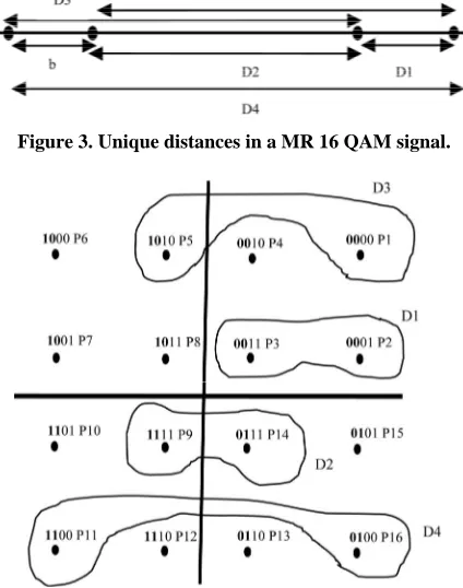
(k = {1,2,3}), which areequally spaced. To achieve multiresolution, we need to introduce unequally spaced points as shown in Figure 3, I would be in the set {–2 – b, –2 + b, 2 – b, 2 + b}. (Note that for, b = 1, we have the SR case.) This results
differ-ences:
x 2b, (2 – b), , (2 b), resulting in k vary-
ing over {b, 2 – b, 2, 2 + b}. In general, for M-array sig-
nals, k varies in the set
b, 2b, ,
M 1
b
whichresults in M – 1 unique distances between signal
sym-bols.
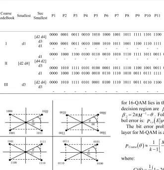
The codebook design is then based two concepts: 1) First Group the points, so that intra-group Euclidean distance is less than inter-group Euclidean distance 2) Second map the points according to the Gray code fine-channel digital bit mapping,
a) Arrange the euclidean distances diin increasing
or-der. Each di corresponds to a Di.
b) Three groups are possible for coarse codebook, as shown in Figure 4. In a group, the intra-group distance must be chosen the minimum one. For coarse data error probability, intra-group Euclidean distance does not ma- tter. Note that possible intra-group distances for M = 4
[image:4.595.316.528.96.365.2]cases are {(d1, d1), (d2, d4), (d3, d3)}.
Figure 3. Unique distances in a MR 16 QAM signal.
Figure 4. Three coarse codebooks for MR-16-QAM. For each codebook, coarse information is represented by closed circle.
c) For each coarse codebook, two fine codebooks are possible. They are chosen on the basis that the points with second smallest distance from each other.
The Codebook for two-layered MR-16-QAM data with two bits in each layer is given in Table 2:
3.1.3. Performance of MR-MQAM
The OFDM MR-modulation have the desirable property that the probability of the symbol error of the coarse layer is unaffected by the error in the fine layers. The high profile base layer video source stream is modulated onto OFDM-carriers using Gray-coded QPSK modula-tion, every two binary symbols are mapped into one QPSK symbol, the QPSK signaling constellation is then converted to a non-uniform 16-QAM signal constellation by splitting each point in the QPSK constellation into four points, each of which is rotated away from the original QPSK point by an angle , as illustrated in Figure 5. The result is a non-uniform 16-QAM signal constellation with signal at angles in the first quadrant at
, , π ,π ,
each point of the 16-QAM is split into four points, each of which is rotated by the same amount from the 16-QAM points.
Table 2. Code book for two-layered data with two bits in each layer. First bits represent coarse data. Euclidien Distance affecting performance of : Coarse
CodeBook Smallest Sec
Smallest P1 P2 P3 P4 P5 P6 P7 P8 P9 P10 P11 P12 P13 P14 P15 P16
C F
I d1
[d2 d4] d3 d1 0000 0000 - 0001 0001 - 0011 0011 - 0010 0010 - 1010 1000 - 1000 1010 - 1001 1011 - 1011 1001 - 1111 1100 - 1101 1110 - 1100 1111 - 1110 1101 - 0110 0111 - 0111 0110 - 0101 0100 - 0100 0101 - Min (d2,d4) d3 d1 d1
II [d2 d4] d1 [d4 d2] d3 0000 - 0000 1000 - 1010 1100 - 1111 0100 - 0101 0110 - 0100 0010 - 0001 1010 - 1011 1110 - 1110 1111 - 1100 1011 - 1001 0011 - 0011 0111 - 0110 0101 - 0111 1101 - 1101 1001 - 1000 0001 - 0010 d1 d3 [d2d4] [d2d4]
III d3
d1 [d2 d4] d3 0000 0000 - 1000 1010 - 1100 1111 - 0100 0101 - 0010 0001 - 0110 0100 - 1110 1110 - 1010 1011 - 0011 0011 - 0111 0110 - 1111 1100 - 1011 1001 - 1101 1101 - 0101 0111 - 0001 0010 - 1001 1000 - d1 Min (d2,d4) d3 d3
Figure 5. Signal constellation for MR 16-QAM.
the enhanced layer data (fine data). The relative prob- ability of the error for the two message streams are con- trolled by varying the modulation parameter from
π
0 to
4 called also the offset angle. To derive the error
probability for data mapping to different resolutions of the signal constellation, we have followed [9]. The noise is modeled as stationary Gaussian noise with one sided spectral density 0. If is the symbol energy for PSK, then S NN0 determines the symbol error prob- ES ability. The error bounded for uniform QPSK, 4-QAM, 16-QAM and 64-QAM constellation are special case
E
with 0, π, π, and
8 16 6
π
4. For a fixed value of
0
S
E
N , the probability of bit error for the coarse layer
increases while the probability of the fine layer decrease, the offset angle is increased form 0 to π
64. The symbol error region for the coarse layer (basic message)
for 16-QAM lies in the first quadrant. The boundaries for decision region are 1
1 2πM
, and 1
2 2πM
. Following [9], the probability of sym-bol error is: Pi s,
Ej
L0Ci
2 Ci
1The bit error probability for the high profile coarse layer for M-QAM is approximated by:
Coarse 1 2 2π 2π
1
M
C C
P
k M M M
(1)
where:
sin( ) 2 0 1( ) 1 2 2 sin 4
1 exp 1 2 cos( ) d 2
π
S
S
e
C Q e
Q y y y 0 S S E e N
, ESbit energy
0
2
N : Two sided power spectral density of the stationary
AWGN
2k
M , and
2
1
d 2 2π x
y
Q x
e yFor the enhanced fine layer the upper bound for the probability of bit error is given by:
fine
1 4π
2
P C
M C
(2)
3.1.3.1. Probability of Error of 2 Layers 4-QAM:
coarse 2 1
1
π π
2 C C
P
Which simplify to: PcoarseQ
2 cose1
for M = 4, for the high resolution layer, the probability of error is according to Equation (2)
fine 2 2 2
1 π 2 sin
2
P C C Q e
3.1.3.2. Probability of Error of 2 Layers 16-QAM A 16-QAM constellation can be see as a two layer mul-tiresolution constellation of two QPSK constellations (Figure 5), using the Equation (1) , the probability of the coarse base –layer of the nth channel for the 16-QAM is given by:
coarse 1 7 π 5π
3 8 8 8
1 7 π 5π
3 8 8 8
1 7 π 5π
3 4 8 8
π 5π
8 8
i i
i i
i i
i i
C C
P
C C
C C
C C
We use the fact that
5π 5π π
sin sin cos 8 8 8
And sin
sin
cos -cos
sin And
5π π
cot tan ,
8 8
5π π
cot tan
8 8
And
1 2Q x( )
1 2Q(x)
0which yield : coarse sin π
8
i
Q e
P
.
This is the probability of the 4-PSK signal constella-tion.
The probability of error for the fine additional message is according to (2):
fine
7 π π
8 4 4
7 3π 5π
8 4 4
i i
i i
P C C
C C
3.1.3.3. Probability of Error of 2 Layers 64-QAM A 64-QAM constellation can be see as a two layer
mul-tiresolution constellation of a coarse QPSK constellation, and a 16-QAM fine constellation (Figure 6), or as a three layers multiresolution constellation of three QPSK mod- ulations. In the case of two layers multiresolution, and using the Equation (1), the probability of the base coarse layer is:
coarse
1 7 π 5π
3 8 8 8
1 7 π 5π
3 8 8 8
i i
i i
C C
P
C C
The probability of error for the fine additional message is according to Equation (2) is:
,
7 π π
8 4 4
7 3π 5π
8 4 4
i b i i
i i
C C
P
C C
3.2. OFDM Time-Frequency Multiresolution The general principal of OFDM system is to achieve high speed data throughput by using multiple orthogonal car- riers for the transmission of data. There are a number of ways by which the OFDM system can be implemented. Fourier OFDM is one of them, but multiresolution OFDM have recently emerged especially wavelet as an interest- ing OFDM system.
In Fourier OFDM, symbol consists of N subcarriers
separated by a frequency distance f . The total system
bandwidth B is divided into N equidistant sub channels
with all subcarriers being mutually orthogonal within a time interval T 1 f . The OFDM signal in the time
domain is
12π
0
1 N , 0 j ft n n
x t X e t
N
T
(3)
To obtain the discrete time representation, the signal
x(t) has to be sampled. The sampling time needs to be
twice the bandwidth that is t 1 1
B N f
[image:6.595.341.506.163.222.2] so that the
[image:6.595.60.264.272.583.2] [image:6.595.348.489.601.723.2]signal can be recovered, the sampled signal is given by:
1 2π
0
1 N , 0,1, j kn N
k n
n
x x e k
N
N1 (4)
Equation (3) represents an N point inverse discrete Fourier transform (IDFT) of the input symbols xn.
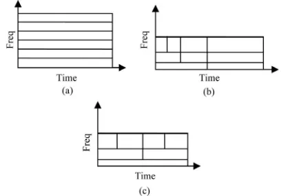
These inputs symbols represent digitally modulated complex data. The IDFT can be implemented using the inverse fast Fourier transform (IFFT) algorithm. The re- presentation time/frequency is depicted in Figure 7(a).
x
nIn the multiresolution (wavelets) OFDM system, the IFDT and the FDT are replaced by the IDWT and the DWT. The main advantage of wavelet OFDM over Fou- rier OFDM is the use of the time-frequency multiresolu- tion.
There are two general approaches to implement OFDM wavelet transforms [10]. The first is denoted as classical wavelet. The second method uses full decomposition and recomposition trees, and is called Wavelet Packet.
In the classical wavelet analysis the signal is coded us- ing a recomposition tree. The transmitter first splits the data sequence, filters each of the subsequences to create the resulting OFDM symbol. The OFDM sequences are then processed in a serial fashion for transmission. This approach leads to the time/frequency representation shown in Figure 7(b), where each block represents a single data symbol. Each of these blocks has the same area, but symbols mapped to higher frequencies have shorter time durations. The data rate is adapted to the carrier frequ- ency as symbols occupy different periods of their as- signed sub-carriers. One can map the coarse modulated symbol of the MR constellation to coarse coefficients carriers frequencies (i.e. QPSK base layer symbols car-
rying high profile unit to more rugged carriers where the spectral efficiency is not a concern), and the fined modu- lated symbol of the MR constellation to fined coeffi- cients carriers (i.e. 16-QAM symbols to the fine carriers
frequencies). Multiresolution OFDM wavelet do not need cyclic prefix for synchronization which leads to a better symbol rate.
In the wavelet packet approach, the time/frequency representation leads to the figure shown in Figure 7(c). This approach is not optimal for the multiresolution be-cause the block has the same area.
3.2.1. Spectral Efficiency of Multiresolution OFDM Channels
In most digital communication systems, the available channel bandwidth is limited, one of the most important feature of multiresolution OFDM is it spectral efficiency. It is then important to determine the spectral content of the digitally multiresolution modulation and multiresolu- tion OFDM modulated signal. From theory we know that power spectral density is used to determine the channel bandwidth required. We can then determine the channel efficiency of the multiresolution OFDM.
Figure 7. (a) Single-resolution (Fourier) OFDM symbol; (b) Multiresolution classical wavelet OFDM symbol; (c) Mul- tiresolution packet wavelet OFDM symbol.
Average Energy of MR-OFDM Channel
In [11] it has been shown that the average power of a single M-QAM constellation is equal to the average en- ergy of one of the quadrants.
The number of symbols in each of the quadrant is M/4,
for each symbol i, the energy is given in term of its
coordinates( , )x yi i , Ei
2
i i
E x yi2, the average energy is:
4
1 M
2 2
1
4
sq i i
i
E x y
M
, the number of symbol in each of the quadrate is:
4
P M . The symbols have coordinates ( , )x yi i ,
where
0 0 0 01 3 5 2 1 , , ,...., 2 2 2 2
i i
p
x y d d d d
,
the average energy for a squared constellation is
2 2
0 0
2
1 1
2 0
1
2 1 2 1
2 2
1
1 6
P P
avg
m n
d d
E m
P
d M
n
For the cross constellation, it has been shown [11] that:
2 0
2 0
1 40 1 for 3 6 32
1 31
1 for 3 6 32
avg
d M k
E
d M k
The average energy of the coarse base layer dedicated to the nth sub channels can be determined according to
the number of the two bits symbols which are located in the first quadrant. For MR-QAM the average energy of the base layer is:
2 01 1
6
lp
avr d M
E
(5)For the fine enhanced layer the number of additional bits symbols in each quadrant is
2k
M
N . The average
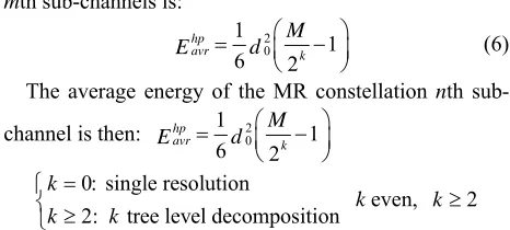
[image:7.595.320.524.85.227.2]mth sub-channels is:
2 0
1
1 6 2
hp
avr k
M d
E
(6) The average energy of the MR constellation nth sub-
channel is then: 2 0
1 1
6 2
hp
avr k
M d
E
0: single resolution
2: tree level decomposition
k
k k
k even, k2
where k is the number of bits which determine the level
of multi-resolution in the constellation and the distance is arbitrary.
0
The total average energy of the MR-QAM is the total energy of the coarse base layer plus the fine enhanced layer which is:
d
2 0
1 1
1 1 for even 2 6 2
N N
Tot
avr avr k
n k n
M
k d
E E
From Equations (5) and (6), we have:
1 2
MR k SR
E E
. (7) Note that for 0, k EMR ESR.
3.2.2. Channel Capacity of MR OFDM Channel The capacity of the band-limited AWGN MR nth chan-
nel is: 2
0
log 1 M MR MR
C E
C W
W N
Where W is the
bandwidth, and N0 is the energy of the noise, hence:
0
1 2WC
E C N
W
.
For the same channel bandwidth W and using Equation
(7), we have:
2
2 1 log 1
2
SR M
MR k
SR
C
C W
C W
C
(8)
where SR is the capacity of the single resolution con-
[image:8.595.55.288.91.196.2]stellation. Figure 8 is the plot of Equation (8) for k = 0, 4, C
Figure 8. Capacity of MR vs. SR channels.
and 8.
For k = 0, we have CMR CSR.
For k = 8, we have CMR 90%CSR.
Spectral Efficiency of MR OFDM Channel
According to [12], the band pass filters have the band-width:
π 0 is the number of channels
2 2
p
W p L L .
The efficiency of the bandwidth usage of the nth channel is:
1 2
log 2p
R
M W
[image:8.595.89.255.591.719.2] (9) where Rlog2k.
Table 3 shows the spectral efficiency for the single and a multiresolution 16-QAM and 64-QAM. It is twice efficient in the case of a double layer MR 64-QAM, and three times in the 3 layers case.
3.3. Experimental Results and Discussion
In this work, we have focused on the DVB-H 4K mode standard [13] intended for mobile reception of standard definition DTV. First we have classified the NAL unit type into two layers: SPS and PPS as highly prioritized units, their identification in the NAL stream is as follows: From the test. 264 file generated by the JM 11 encoder there is 31104 bits, in which 216 are high priority sub- stream and it consists mainly of NAL unit type 7 which is SPS, and NAL unit type 8 which PPS, JM1l decoder is zero tolerant for these loss of these units, the left sub- stream is treated as low priority, The OFDM system is specified for 8 Mhz channel spacing, the parameters are the same except for the period T, The two independents H264 streams are mapped on to the multi-resolution mo- dulation signal constellations to generate symbols con- stellations in the baseband channels (Figure 9).
In the pass band domain, the transmitted OFDM signal is organized in frame of duration TF and consists of
7771 OFDM symbols. Each OFDM symbol is consti-tuted by a set of K = 3408 carriers in the 4K mode and
transmitted with duration Ts, A useful part with duration
and a guard interval with a duration
TU TD. The sub-
carrier 1 is 7.61/2 MHz to the left and sub carrier 3408 is 7, 61 to the right. Figure 10 shows the PSD of the 64-
Table 3. Spectral efficiency single vs. multiresoltion OFDM.
Modulation Spectral Efficiency (bits/s/Hz)
SR-16 QAM 4
SR-64 QAM 6
MR-16 QAM 8
MR-64 QAM two levels 12
[image:8.595.310.538.648.737.2]Figure 9. Multiresolution constellation for H.264/AVC file input.
Figure 10. PSD of (a) single; (b) multiresolution 64-QAM modulation OFDM over DVB-H 4K channel and H264 file input; (c) wavelet OFDM.
QAM single and multiresolution modulation for DVB-H 4K mode with layered H264 file input.
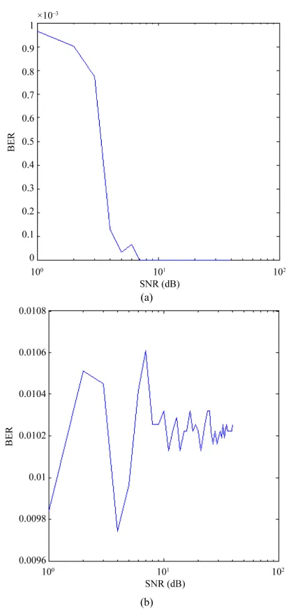
Figure 11(a) is the plot of BER vs. SNR for a two level 64-QAM multiresolution modulation in a SNR en- vironnement, and (b) is the performance of a two level 64-QAM multiresolution modulation in a Raleigh fading environnement.
4. The Multiresolution Turbo Code System
Multiresolution analysis via decomposition is an impor- tant tool in signal analysis. An analogous framework for the multiresolution analysis of finite-length sequences from aritrary field was defined in term of the generator matrices of convolutional code [14]. Convolutional codes are core constituent for turbo coding and can be treated using both the multirate analysis because of their con- volution property and the finite state machine analysis. In this work we will use both analysis for understanding the behavior of multiresolution and decomposition of convo- lutional code and hence the PCCC and the Turbo codes.In theory a coded stream is a convolution of the input stream with encoder’s impulseresponses:
0
j j
i k k i
k
y h x
where xi is an input sequence, j
i is a sequence from
output and
y
j
h is an impulse response for output j. A
convolutional encoder is a discrete linear time-invariant system. Every output of an encoder can be described by its own transfer function, which is closely related to a generator polynomial. The Transfer function for the recursive encoder of Figure 7 used in [15] is:
1 2 31 4
1
1
D D D D
H z
D
4
Define m as: m max polydeg Hi 1
z
where for
any rational function
p z f z
Q z
,
polydeg (f) = max(deg(p),deg(Q))
Then m is the maximum of the polynomial degree of
the Hi 1
z
, and the constraint length is defined as: k =
m + 1. The constraint length of the encoder of Figure 12 is 5.
Let the input to the encoder at time K is a bit , and
the corresponding codeword is the bit pair ( , ) where:
k
d
k
u vk
1
1 1 1
0
mod2 and 0,1
k
k i k i
i
u g d g
1
2 1 2
0
mod2 and 0,1
k
k i k i
i
v g d g
[image:9.595.82.263.267.695.2](a)
[image:10.595.67.277.78.515.2](b)
[image:10.595.76.268.553.639.2]Figure 11. Plot of BER vs. SNR of multiresolution OFDM. (a) SNR channel; (b) Rayleigh channel.
Figure 12. SR [37,21] recursive convolutional code.
1 g1i and G2 g2i
G
dk
are the code generators, and is represented as a binary digit. This encoder can be visualized as a discrete-time finite impulse response (FIR) linear system, and in the case of recursive constituent code; it is equivalent to an infinite impulse response filter (IIR).
4.1. Polyphase Decomposition
The polyphase representation has been an important ad-vancement in the mulitrate signal processing, which per- mits great simplification of theoretical results and alleged complexity [12].
Consider a coder with generator function:
1
0
k
n k
i
u h n z
By separating the even numbered coefficients of h(n)
from the odd numbered ones, we can write:
1 1
1 2
0 0
2 1
k k
n n
k
i i
u h n z z h n z
Defining:
1 1
0 1
0 0
2 , 2 1
k k
n n
i i
u h n z u h n z
Therefore, we can write:
2 1
20 1
k
u u z z u z
In general, we have:
1 1 0
M
l M k
l
u z u z
where 1 1
0
k
n l
n
u e n z
With
( )n h Mn l( ) , 0 l M 1
el
the signal y(n) is obtained by interlacing y0(n) and 1 that is, is:
( )
y n
2).
( )
y n 1 0 1 0 1 0
Which is a time-multiplexed version of the output of .
(0) (0) (1) (1) (2) (
y y y y y y
0( ) andz 1( )z
R R
4.2. Multiresolution Transfer Function
Finding the free distance of a PCCC and therefore of a Turbo code is complicated by the fact that these code are time varying due to the interleaver.
In the case of single resolution, many approaches for the evaluation of the transfer function of the PCCC have been proposed in the literature. The two most famous are those of Disalvar et al. [16] and Benedetto and Montorsi
[17,18]. In this paper the methods in [17,18] have been followed.
Let
, ,
jwjn k
A w z n
A Zse-quences of the convolutional code generated by concate-nating n error events with total information w.
wjn
A is the number of codewords with information bit
weight w, parity-check weight j and number of
concate-nated error n, and Z in the dummy variable.
In multiresolution coding, the dummy variable of the high coder is h
Z and the low coder is Zl, where h is
the high parity-check weight and l is the low parity-check
weight by using the property of “Devide and Concert” of polyphase decomposition, we can decompose the convo- lutinal code to its components, the free distance of the CC is the sum of the free distance of it components.
The parity-check enumerating function of the sequ- ences of the multiresolution code can be written in matrix form as:
Low
Multires High T
A A A
where AHigh and ALow are respectively the enumerating function of the high level component and low level component. The multiresoltion conditional weight enu-merating function can be written as:
Low High Low HighMultires , ,
, , ! c T h o n T h o N
w z A w z w z
A A
n
N A w z w z
A n , w w
The conditional weight enumerating function of the two
2 ,N N constituent equivalent block of the twoPCCC code is defined as:
2
, ,
C
CP A w z
A w z
N w
4.3. Multiresoltion Performance Bound
The input sequence is restricted to thengh N, where N
correspond to the size of the interleaver of the PCCC. With finite length input sequences of length N. A
(2,1, ) convolutional code may be viewed as a block code with 2N codewords of length (2,1, ) . For the
multiresolution case and following [18], we get for the conditional weight enumerating function:
21 2 2
Highres Lowres Multires 1 2 ! , . ! !
P n n w T
C w z w N
A
n n
A .A
For large N the approximation 1 2 max is used
and the asymptotic bound for the bit error probability:
n n n
max 2 High max min 02 1 2
high max
2
low Low max
!
( ) , , .
!
, , RC EbN
N
n w w
b
w w
w z e
w
P e w N W A w Z n
n
w Z n
A
where denotes the minimum information weight in
the error events of the CC.
min
w
For nonrecursive convolutional constituent encoder, we have wmin 1 and nmax w , and A w Z w( , , )
and the asymptotic bound becomes:
(1, ,1)w
A Z
High 0 1 2 high 1 1 2 low Low( ) 1, ,1 .
1 ! 1, ,1 RC EbN
w N N w w b w w
w z e
N
P e W A Z
w Z A
For the most favorable case (w = 1) the bit error
prob-ability is independent of N.
For recursive encoders wmin has been shown to be equal to 2 and max
2
w n
, Using the same approxima-
tion as in [18], we have: min high
min high
high(2, ,1)
1 z z z A Z z
and
min low min low low(2, ,1)
1 z z z A Z z
And the asymptotic expression of the upper bound yield to:
high
low
min min 0 2 1 1 high low min min 2
( ) 2
2 2
1 2 1 2
RC EbN
N
b k
z z
w z e
k
P e k N
k
H z z
H H
The interleaver gain for the PCCC of the constituent encoders goes as 1
N , the interleaver size N can be split
in high resolution and low resolution components. The effective free distance of the multiresolution PCCC can be defined as:
high low free,multi=2 2 min 2 min
d z z
From the above equation we can choose the encoder decomposition so that the free distance of the high level encoder which protect the sensitive information greater than the free distance of the low level encoder
which protect the irrelevant information.
high min z low min z
Example: Berrou Turbo Code
Consider the turbo code of [15], the generator matrix of the systematic recursive convolutional code [37,21] is:
2 3 4
4 1
1,
1
SR
D D D D
G D
Figure 13. HR [7,5] recursive convolutional component code.
2
2 1 1,
1
H
D D
G
D
and 2
1 1,
1 L
D G
D
for the low
resolution constituent encoder [6,5] (Figure 14), up on solving the state equations for the ratio E
S
X
X of the aug-
mented state diagrams for the high level and low level encoder, the transfer function for the HR encoder is:
4 4 6 5 3 3 2 3
High 2 3 2 3 2
( )
( , , )
( ) (
N J D D N J N J
T D N J
D N NJ
J N J J
D
) 1
Setting J= 1, the free distance freeLowAnd for the transfer function of the LR encoder is: 5
d
2 4 6 4 2 3 2 4
Low 2 2 3
( , , ) 1
N J D D N J N J
T D N J
J NJD NJD NJ D NJ D
Setting J= 1, the free distance freeLow , the free distance of the (37,21) code is therefore equal to 7.
2
d
Figure 15 shows the multiresolution state diagram of the (37,21) code where the two output bits are the HR output and the LR output of the multiresolution encoder. Figure 16 shows the theoretical bound for SR (37,21) Turbo code and its MR (7,5) and (6,5) components. 4.4. Generalisation of Multiresolution
Decomposition
The UEP capability of a convolution encoder is mea- sured by the effective free distance vector of length k (the number of possible UEP protection levels). If all entries in the free distance vector are equal, then the en-coder possesses the equal error protection (EEP) capabil-ity [19].
In theory we consider the codeword M L
X UG
1
M
, where is the input word and
1 kU u u
X
xxn
isthe codeword, the error vector is defined as:
O M
eX X where X0 is the distorted codeword. If the decoding is done according to free distance, then if the ith symbol is protected against error of class i
whereas the j-t symbol is protected against error of class
E
j
E where i j, then the -th symbol can be de-
coded correctly if E E
xi
j iwhereas codewords pro-
tected by class E t
E
j
E is distorted. In general if Ej is a set
[image:12.595.340.503.87.165.2]of distortion codeword vector, the magnitude of which is
Figure 14. Low R [6,5] recursive convolutional component code.
not higher than tj, then the i-th symbol of the codeword
is protected against tj errors. The structure of concate-
nating systematic convolutionel code used in PCCC al- low the generation of new UEP codes.
The concatenation of matrices can be used to create new correcting codes; using matrices the fol- lowing matrices are generated: 1 2
,
G G
1 2
A G G And
2 2 1
0G
G
B G
It is evident that if l1 and l2 are linear
n k d1, ,1 1
and
n k d1, ,1 1
code then the concatenation of type Agenerate a
n1n k2 d 1d2
1 k
G 1
, k2, , while the con- catenation B will generate a .
d
n n
1 2 2 dd1
A particular switch in the rows of 1 will generate a code which will protect two groups of symbols: the first group by the free distance and the second, k ,
1
dd d2 one by dd1. The matrice 1 0 2
1 2
G G
B
G G
generates
a
n1n k2, 1
code with the minimum distance d =
min d d1, 1d2 The matrix generated using concate-
nating has size:
n1n2
k1k2
and generate a code with the minimum distance dmin
d1d2
, while a
n1n2
max
k k1, 2
matrix generates a code with the minimum distance:min 1 2 1 2
min 1 1 2 1 2
min 2 1 2 1 2
if if and if and
d d d k k
d d k k d d
d d k k d d
In the case of a 3 branches binary tree structure con-volutional code, the generator matrix of the encoder can be written as:
2
2 4
H z
B G z H z
G z G z H z
Corollary:
If mi is the free distance of an encoder of generator matrix n
z
H z , the free distance of its component
2Figure 15. Multiresolution state diagram of the MR (37,21) convolutional code.
Using the result from the corollary, we deduce that the free distance of the second branch in the multiresolution decomposition tree is: min min
And the free distance for the third branch is:
2.
Low High
z z
min min
2 Low High 6
z z .
The distance of the branches decreases as the level of decomposition in the tree structure.
If the matrices G(z) and H(z) are appropriately
de-signed, then, the encoder tree structure system produces perfect reconstruction that is X nˆ ( ) X n( ), in this case
we get a quadrature Mirror coders (QMC), that is the two coders have equal free distance and generate the same protection, the generator matrix satisfies the power sym- metric condition:
Figure 16. Theoritical bound for SR (37,21) TC and its MR
(7,5) and (6,5) components. H z H z( ) ( )H( ) ( ) 2z H z
where H z( )is the complex conjugation of H(z).
Proof: Under this condition, and if the remaining coders are
chosen according to: If min is the minimum free distance of the encoder
with generator matrix
z
H z and degree N, then it coder
component with generator matrix
2H z which has
degree N – 2, therefore the minimum free distance is
. min
z 2
1) ( )G z
z
NH( ) where is the order of ( ).z N H z2) the reconstruction encoder H ( )z H z( ) andG ( )z
R R
Then we have the Perfect reconstruction condition ( Fig-ure 17).
( )
[image:13.595.58.286.440.621.2]Figure 17. A three levels multiresolution decomposition tree code.
Figure 18. Performance of SR Turbo code and its HR and LR components for H.264/AVC UEP.
4.5. Experimental Results and Discussion
The Turbo Code of Berrou [15] is used for single resolu- tion, its component are set with the same parameter with size interleaver 10. The two layered independents H264 streams are protected using different multi-resolution encoders , the HL component TC (7,5) present almost the same performance but at outstanding low cost and pro- tecting the most valuable data (SPS, PPS and IDR) where it counterpart LL TC component (6,5) shows some deg- radation and is suitable for irrelevant data protection (Figure 18).
5. Conclusion
In this work we have investigated a multiresolution lay- ered H.264/AVC OFDM scheme with a multiresolution modulation scheme in it base band domain followed by Time/frequency modulation in pass-band domain for the purpose to increase the performance of the OFDM over- all system. First We have presented a mutiresolution source layered H.264/AVC data partition based on im- portance characteristics and then presented the design of the multiresolution constellation base band and the mul- tiresolution OFDM pass band and showed its substantial
superiority over single resolution in term of probability of bit error rate, channel capacity and spectral efficiency. We have investigated the multiresolution channel coding protection. We showed that the free distance of convolu- tional code is the sum of its multiresolution components, the protection of the multiresolution protection system decrease as we move through the levels of the decompo- sition tree. The free distance also decreased, we have simulated the multiresolution Turbo code for H.264/AVC UEP, and showed its prominent outperformance over the single resolution channel protection.
REFERENCES
[1] K. RamChandran, et al., “Muliresolution Broadcast for
Digital HDTV Using Joint Source Channel Coding,” IEEE Journal on Selected Areas in Communication, Vol. 11,
No. 1, 1993, pp. 6-23.
[2] T. Cover, “Broadcast Channels,” IEEE Transactions on Information Theory, Vol. 18, No. 1, 1972, pp. 2-14. doi:10.1109/TIT.1972.1054727
[3] T. Wiegand, G. J. Sullivan, G. Bjentegaard and A. Luthra, “Overview of the H.264/AVC Video Coding Standard,”
IEEE Transactions on Circuits and Systems for Video Technology, Vol. 13, No. 7, 2003, pp. 560-576.
doi:10.1109/TCSVT.2003.815165
[4] S. Kumar, L. Xu, M. K. Mandal and S. Panchanathan, “Error Resiliency Schemes in H.264/AVC Standard,”
Journal of Visual Communication and Image Representa-tion, Vol. 17, No. 2, 2006, pp. 425-450.
[5] Y. Dhondt and P. de Walle, “Flexible Macroblock Order-ing an Error Resilience Tool in H264/AVC,” Fifth FTW Ph.D. Symposium, Faculty of Engineering, Ghent Uni-versity, 2004.
[6] S. Ueda, H. Shigeno and K. I. Okada “NAL Level Stream Authentification for H.264/AVC,” IPSJ Digital Courier,
Vol. 3, 2007, pp. 55-63. doi:10.2197/ipsjdc.3.55
[7] J. G. Proakis, “Digital Communications,” McGraw-Hill, New York, 1989.
[8] A. S. Saxena, “Embedded Multiresolution Signaling Sch- eme for CPFSK Modulation,” 2003.
[image:14.595.72.273.230.399.2][9] M. Pursley and J. Shea, “Nonuniform Phase-Shift-Key Modulation for Multimedia Multicast Transmission in Mo-bile Wireless Networks,” IEEE Journal on Selected Areas in Communication, Vol. 17, No. 5, 1999, pp. 774-783. [10] M. Lallart, K. Nolan, P. Sutton and L. Doyle, “On-the
-Fly Synchronization Using Wavelet and Wavelet Packet OFDM,” IEEE Signal Processing Letters, Vol. 12, 2005,
pp. 577-580.
[11] H. Holms, M. M. Ghandi and E. V. Jones, “Spectral Effi-ciency of Variable-Rate Coded QAM for Flat Fading Channels,” IEEE Signal Processing Letters, Vol. 12, 2005,
pp. 577-580.
[12] P. P. Vaidyanathan, “Multirate Systems and Filter Banks,” Prentice-Hall, Englewood Cliffs, 1992.
[13] G. Faria, J. A. Henriksson, E. Stare and P. Talmola, “DVB-H: Digital Broadcast Services to Handheld De-vices,” Proceeding of the IEEE, Vol. 94, No. 1, 2006, pp.
194-209. doi:10.1109/JPROC.2005.861011
[14] S. Amir, A. Mehr, K. Nayebi and S. Kasaei, “Multirate Structures for Arbitrary Rate Error Control Coding,” 2003
IEEE International Conference on Acoustics, Speech, and Signal Processing, Vol. 4, 2003, pp. 245-248.
[15] C. Berrou, A. Glavieux and P. Thitimajshima, “Near Shannon Limit Error-Correcting Coding and Decoding: Turbo Codes,” IEEE International Conference on Com-munications, Geneva, 23-26 May 1993, pp. 1064-1070.
[16] D. Divsalar, S. Doliar and F. Pollara, “Transfer Function Bounds on the Performance of Turbo Codes,” TDA Pro-gress Report, Vol. 42, No. 122, 1995, pp. 44-45.
[17] S. Benedetto and G. Montorsi, “Unveilling Turbo Codes: Some Results on Parallel Concatenated Coding Schemes,”
IEEE Transactions on Information Theory, Vol. 42, No. 2,
1996, pp. 409-428. doi:10.1109/18.485713
[18] S. Benedetto and G. Montorsi, “Design of Parallel Con-catenated Convolutional Codes,” IEEE Transaction on Communications, Vol. 44, No. 5, 1996, pp. 591-600.
[19] E. Kuriata, “Creation of Unequal Error Protection Codes for Two Groups of Symbols,” International Journal of Applied Mathematics and Computer Science, Vol. 18, No.


![Figure 13. HR [7,5] recursive convolutional component code.](https://thumb-us.123doks.com/thumbv2/123dok_us/9260013.415482/12.595.88.255.86.165/figure-hr-recursive-convolutional-component-code.webp)
