Computational surface partial differential equations

(1)

University of Warwick institutional repository: http://go.warwick.ac.uk/wrap

A Thesis Submitted for the Degree of PhD at the University of Warwick

http://go.warwick.ac.uk/wrap/57647

This thesis is made available online and is protected by original copyright.

Please scroll down to view the document itself.

(2)

Library Declaration and Deposit Agreement

1. STUDENT DETAILS

Please complete the following:

Full name: ………. University ID number: ………

2. THESIS DEPOSIT

2.1 I understand that under my registration at the University, I am required to deposit my thesis with the University in BOTH hard copy and in digital format. The digital version should normally be saved as a single pdf file.

2.2 The hard copy will be housed in the University Library. The digital version will be deposited in the University’s Institutional Repository (WRAP). Unless otherwise indicated (see 2.3 below) this will be made openly accessible on the Internet and will be supplied to the British Library to be made available online via its Electronic Theses Online Service (EThOS) service.

[At present, theses submitted for a Master’s degree by Research (MA, MSc, LLM, MS or MMedSci) are not being deposited in WRAP and not being made available via EthOS. This may change in future.]

2.3 In exceptional circumstances, the Chair of the Board of Graduate Studies may grant permission for an embargo to be placed on public access to the hard copy thesis for a limited period. It is also possible to apply separately for an embargo on the digital version. (Further information is available in the Guide to Examinations for Higher Degrees by Research.)

2.4 If you are depositing a thesis for a Master’s degree by Research, please complete section (a) below. For all other research degrees, please complete both sections (a) and (b) below:

(a) Hard Copy

I hereby deposit a hard copy of my thesis in the University Library to be made publicly available to readers (please delete as appropriate) EITHER immediately OR after an embargo period of ………... months/years as agreed by the Chair of the Board of Graduate Studies.

I agree that my thesis may be photocopied. YES / NO (Please delete as appropriate) (b) Digital Copy

I hereby deposit a digital copy of my thesis to be held in WRAP and made available via EThOS.

Please choose one of the following options:

EITHER My thesis can be made publicly available online. YES / NO (Please delete as appropriate) OR My thesis can be made publicly available only after…..[date] (Please give date)

YES / NO (Please delete as appropriate) OR My full thesis cannot be made publicly available online but I am submitting a separately identified additional, abridged version that can be made available online.

(3)

3. GRANTING OF NON-EXCLUSIVE RIGHTS

Whether I deposit my Work personally or through an assistant or other agent, I agree to the following:

Rights granted to the University of Warwick and the British Library and the user of the thesis through this agreement are non-exclusive. I retain all rights in the thesis in its present version or future versions. I agree that the institutional repository administrators and the British Library or their agents may, without changing content, digitise and migrate the thesis to any medium or format for the purpose of future preservation and accessibility.

4. DECLARATIONS

(a) I DECLARE THAT:

I am the author and owner of the copyright in the thesis and/or I have the authority of the authors and owners of the copyright in the thesis to make this agreement. Reproduction of any part of this thesis for teaching or in academic or other forms of publication is subject to the normal limitations on the use of copyrighted materials and to the proper and full acknowledgement of its source.

The digital version of the thesis I am supplying is the same version as the final, hard-bound copy submitted in completion of my degree, once any minor corrections have been completed.

I have exercised reasonable care to ensure that the thesis is original, and does not to the best of my knowledge break any UK law or other Intellectual Property Right, or contain any confidential material.

I understand that, through the medium of the Internet, files will be available to automated agents, and may be searched and copied by, for example, text mining and plagiarism detection software.

(b) IF I HAVE AGREED (in Section 2 above) TO MAKE MY THESIS PUBLICLY AVAILABLE DIGITALLY, I ALSO DECLARE THAT:

I grant the University of Warwick and the British Library a licence to make available on the Internet the thesis in digitised format through the Institutional Repository and through the British Library via the EThOS service.

If my thesis does include any substantial subsidiary material owned by third-party copyright holders, I have sought and obtained permission to include it in any version of my thesis available in digital format and that this permission encompasses the rights that I have granted to the University of Warwick and to the British Library.

5. LEGAL INFRINGEMENTS

I understand that neither the University of Warwick nor the British Library have any obligation to take legal action on behalf of myself, or other rights holders, in the event of infringement of intellectual property rights, breach of contract or of any other right, in the thesis.

Please sign this agreement and return it to the Graduate School Office when you submit your thesis.

(4)

Computational surface partial differential equations

by

Thomas Ranner

Thesis

Submitted to the University of Warwick

for the degree of

Doctor of Philosophy

Mathematics Department

(5)

List of Tables

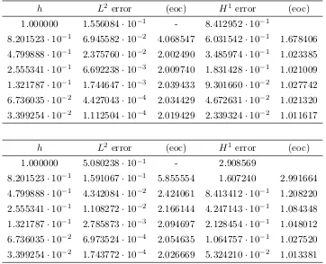
2.1 Error table of the solution of finite element scheme (2.4.4), k= 1 . . 50

2.2 Error table of the solution of finite element scheme (2.4.4), k= 2 . . 51

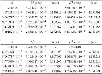
3.1 Convergence for fourth order linear problem . . . 116

4.1 Result for the sharp interface unfitted finite element method on a sphere142

4.2 Result for the sharp interface unfitted finite element method on a torus143

4.3 Result for the method ofOlshanskii et al. (2009) on a torus . . . 144

4.4 Result for sharp interface unfitted finite element method on Dziuk surface . . . 145

4.5 Result for the narrow-band unfitted finite element method on a sphere148

4.6 Result for the narrow-band unfitted finite element method on a torus 149

A.1 Results for surface finite element method on a sphere. . . 174

A.2 Results for surface finite element method on a torus. . . 175

(9)

List of Figures

1.2.1 Example of a triangulated surface approximation of a curve . . . 4

1.2.2 Example of a level set function . . . 5

1.2.3 Example of phase field representation of a curve . . . 7

1.2.4 Example of unfitted representations of a surface . . . 8

1.2.5 Example of a closest point method domain . . . 10

2.3.1 Example of a bulk triangulation. . . 27

2.3.2 Example of simplices with curved faces. . . 31

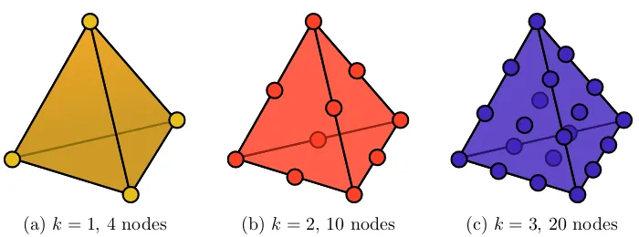
2.4.1 Location of Lagrangian nodes in 3 dimensions . . . 38

2.6.1 Plot of the solution of finite element scheme (2.4.4) . . . 52

2.6.2 Second plot of the solution of finite element scheme (2.4.4). . . 53

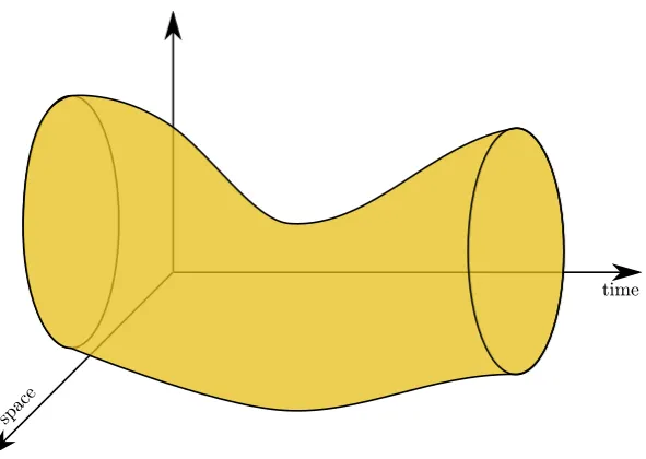
3.2.1 Sketch of space-time domain G_T . . . 57

3.2.2 Sketch of normal and tangential velocities . . . 59

3.3.1 Example of an evolving triangulated surface . . . 72

3.3.2 Example of a lifted triangulation . . . 79

3.6.1 Convergence in energy for Cahn-Hilliard on an evolving surface . . . 117

3.6.2 The decrease in energy for Cahn-Hilliard on an evolving surface . . . 118

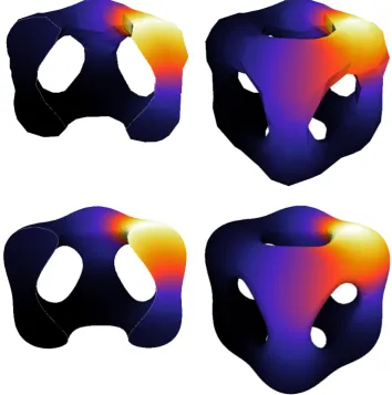
3.6.3 Plot of Cahn-Hilliard solution . . . 119

3.6.4 Example of Cahn-Hilliard on a evolving surface . . . 120

3.6.5 Another example of Cahn-Hilliard on a evolving surface . . . 121

4.2.1 Sketch of polyhedral narrow band about surface. . . 124

4.2.2 Example of the computational domain for unfitted finite element methods . . . 125

4.2.3 Examples of intersection of unfitted computational domain . . . 126

4.3.1 Computational domain for sharp interface unfitted method . . . 130

4.4.1 Example of adaptive mesh for unfitted calculations . . . 140

(10)

A.3.1Example of triangulation of a sphere . . . 158

(11)

Acknowledgments

First, I would like to thank my Ph.D. supervisor, Professor Charles M. Elliott. He

has introduced me into this field of research and provided me with the knowledge

and skills to be able write this thesis. It is an honour to work with not only a world

renowned academic but also a genuinely thoughtful, generous and kind person.

I would also like to thank Bj¨orn Stinner and Andreas Dedner for providing

their expertise in scientific computing, especially for their help with theALBERTA

and DUNE software libraries. I have been lucky to have Andrew Stuart to mentor

my progress which has provided helpful and alternative perspectives on my work and

career. Scientific discussions with Klaus Deckelnick and Gerhard Dziuk have proved

also to be incredibly useful: The opportunity to speak with original investigators

of numerical methods for surface partial differential equations has proven to be

extremely beneficial. I am also grateful for the comments of my examiners, Andrew

Stuart and Endre S¨uli, which have greatly improved my thesis.

On a practical level, I wish to give thanks to the EPSRC for funding my

studies and the Centre for Scientific Computing for providing the necessary

com-putational facilities for my work. In addition I wish to thank the European

Sci-ence Foundation, the Isaac Newton Institute, the London Mathematical Society,

the Mathematisches Forschungsinstitut Oberwolfach, the Oxford Centre for

Collab-orative Applied Mathematics, the Society for Industrial and Applied Mathematics

and the Wales Institute of Mathematical and Computational Sciences for various

travel and conference grants. I would also like to thank Martin Rumpf at Universit¨at

Bonn and the Hausdorff Center for Mathematics for hosting my visits to Bonn.

(12)

Damon McDougall, Dave Moxey and Sebastian Vollmer for contributing to a lively

and enjoyable atmosphere in B2.39, making it a pleasant space to work. It is fair to

say that I would not have been able to perform any of the computations in this thesis

without their help. I also wish to thank Andrew and Damon, along with Andrew

Lam and David McCormick, for taking on the intimidating task of proofreading

my work. A special thanks go to my various housemates and people I have played

hockey with over the last four years.

I must thank my parents, and the rest of my family, for their unconditional

support, love and encouragement: it has meant a great deal to me. Although, they

will always say they do not really understand what I do, I hope they at least enjoy

the pictures. The final, and most important, thanks goes to my girlfriend, Victoria:

(13)

(14)

Declarations

I declare that this thesis contains entirely my own research, conducted under the

supervision of Charles Elliott, except where otherwise stated. It has not been

sub-mitted for a degree at any other university. It has not been subsub-mitted for award

at any other institution or for any other qualification. The material in chapter two

is from a paper published in the IMA Journal of Numerical Analysis (Elliott and

Ranner 2013). The material in chapter three is joint work with Charles Elliott and

chapter four is joint work with Charles Elliott and Klaus Deckelnick. Much of the

introductory material is taken from the work of Dziuk and Elliott (2013b): This

(15)

Abstract

Surface partial differential equations model several natural phenomena; for example in fluid mechanics, cell biology and material science. The domain of the equations can often have complex and changing morphology. This implies analytic techniques are unavailable, hence numerical methods are required. The aim of this thesis is to design and analyse three methods for solving different problems with surface partial differential equations at their core.

First, we define a new finite element method for numerically approximating solutions of partial differential equations in a bulk region coupled to surface partial differential equations posed on the boundary of this domain. The key idea is to take a polyhedral approximation of the bulk region consisting of a union of simplices, and to use piecewise polynomial boundary faces as an approximation of the surface and solve using isoparametric finite element spaces. We study this method in the context of a model elliptic problem. The main result in this chapter is an optimal order error estimate which is confirmed in numerical experiments.

Second, we use the evolving surface finite element method to solve a Cahn-Hilliard equation on an evolving surface with prescribed velocity. We start by deriv-ing the equation usderiv-ing a conservation law and appropriate transport formulae and provide the necessary functional analytic setting. The finite element method relies on evolving an initial triangulation by moving the nodes according to the prescribed velocity. We go on to show a rigorous well-posedness result for the continuous equa-tions by showing convergence, along a subsequence, of the finite element scheme. We conclude the chapter by deriving error estimates and present various numerical examples.

(16)

Chapter 1

Introduction

1.1 What is a surface partial differential equation?

Surface partial differential equations arise in a variety of natural applications. In this thesis we will study partial differential equations posed on both stationary and

evolving surfaces both mathematically and numerically. The framework will be

geometric since the domains in which these equations are posed will be curved. A surface partial differential equation is a partial differential equation whose

domain is ann-dimensional curved surface Γ living inRn+1. We contrast this with

geometric partial differential equations which are partial differential equations for the evolution of a surface.

This means replacing the regular Cartesian derivatives with tangential

gra-dients which are intrinsic to the surface; seeAppendix A for full definitions. As an example, we consider the surface Poisson equation:

−∆Γu=f on Γ. (1.1.1)

Here ∆Γ is the Laplace-Beltrami operator, the surface equivalent to the Laplace

operator. This will be the simplest model equation we consider. We may also

consider a more general elliptic equation on a surface:

− ∇_Γ·(A∇_Γu) +B · ∇_Γu+Cu=f on Γ. (1.1.2)

Here∇_Γis the tangential gradient and∇_Γ·the tangential divergence. This equation

is elliptic if the diffusion tensorA is positive definite on the tangent space to Γ. In general, this means thatA will vary in space, although the scalar matrixA=αId

(17)

equation:

ut= ∆Γu on Γ

u(·,0) =u0 on Γ.

(1.1.3)

Throughout this thesis, we will assume that the boundary of Γ is empty, although

this is not a restriction on our methods. In the case that ∂Γ is not empty, we may consider standard boundary conditions alongside (1.1.2) or (1.1.3); for example:

u=g on∂Γ or ∂u

∂µ =g on ∂Γ. (1.1.4)

Here µ is the outward pointing unit conormal to ∂Γ — normal to ∂Γ but tangent to Γ. SeeAppendix Afor more precise definitions.

Alternatively, one can also consider partial differential equations on an

evolv-ingn-dimensional surface{Γ(t)}fort∈[0, T]. A prototypical example is the evolv-ing surface heat equation:

∂•u+u∇_Γ·v−∆Γu= 0 on Γ(t) u(·,0) =u0 on Γ(0).

(1.1.5)

Here,∂• is the material derivative andvthe material velocity of Γ(t). The material derivative,∂•u, is an intrinsic derivative on the space-time domain of the equation measuring the rate of change of u along the flow of the surface; see Section 3.2.1

for more precise details. The evolution of the surface may be given or need to be

computed as the solution of a geometric partial differential equation, which may

depend on the evolution of the field uon the surface:

v=g(x, ν, H, u) on Γ(t).

Hereν is the unit normal vector field to Γ(t) and H is the mean curvature of Γ(t). A simple example is given by forced mean curvature flow:

v=V ν V =−H+u on Γ(t).

For a review of computational methods for geometric partial differential equations seeDeckelnick, Dziuk and Elliott(2005).

Often in applications, domains have complex evolving morphology so

ana-lytic methods are unavailable. In this thesis, we derive and analyse computational methods to solve surface partial differential equations. In practice, this means

(18)

which are of this fully coupled evolving form. In the problems presented in this

thesis, we will assume either a given velocity or no velocity. Analysis of methods for surface partial differential equations coupled to geometric evolution laws is beyond

the scope of current research methods.

1.2 Computational methods for surface partial

differ-ential equations

There are several methods designed to solve partial differential equations given in the literature. They fall into two broad categories: either using an explicit or implicit

representation of the surface. The first approach uses a parametric viewpoint and

approximates the surface using a triangulated surface and performs calculations on the discrete surface. The second category embeds the surface into Cartesian space

and uses implicit representations of geometric quantities. In this section, we give a

summary of a selection of these methods. As well as the given references, the review ofDziuk and Elliott(2013b) gives more details on many of these methods and their

motivation.

The history of triangulated surfaces, and perhaps finite element methods in general, can be traced back to the work of Schellbach (1851) who proposed using

a triangulated surface to solve Plateau’s problem of determining the surface of a

minimum area enclosed by a given closed curve. The first modern work to use a polyhedral approximation of a surface is due to Nedelec (1976) who considered a

problem involving a surface integral. He constructed an exact triangulation of the

surface consisting of curved simplices. To calculate the surface integral he used a high order quadrature rule to approximate the area element using a parameterisation

of the surface. Baumgardner and Frederickson (1985) looked at ways to construct

such exact triangulations.

The seminal work of Dziuk (1988) introduced what is now known as the

surface finite element method. This method uses a polyhedral approximation of

the surface consisting of planar triangles and then solves variational forms of partial differential equations using a finite element method. Integrals on each element can be

performed exactly since elements in the mesh are no longer curved, however errors arising from approximating the surface in this way are of the same order as the

standard planar interpolation error. This means the error is of optimal order with

respect to the dimension of the surface. The method allows conventional software to be easily adapted for solving surface problems: The only difference is now that

(19)

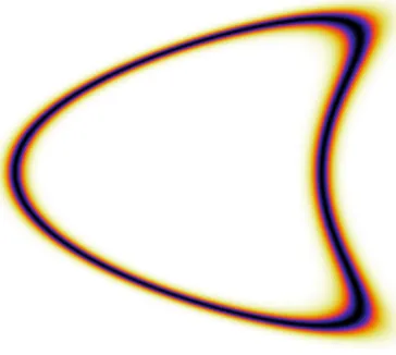
Figure 1.2.1: An example of a triangulated surface approximation of a curve Γ =

{x∈_R2 : Φ(x) = 0}with Φ(x1, x2) = p

(x1−x22)2+x22−1.

Higher order surface approximations have been developed by others

includ-ing Heine (2005) and Demlow (2009). A reliable and efficient error estimator for

adaptive calculations is given byDemlow and Dziuk (2007). The surface finite el-ement method was extended to linear and non-linear parabolic equations by Dziuk

and Elliott(2007b). This approach was used byBarreira(2009) to solve a variety of

non-linear problems on surfaces andDu, Ju and Tian(2011) have given an analysis of a fully discrete approximation of a Cahn-Hilliard equation posed on a triangulated

surface.

Other discretisations of surface partial differential equations on stationary surfaces have used a triangulated surface as the computational domain. Dedner,

Madhavan and Stinner (2013) have studied a discontinuous Galerkin method for

solving a Poisson equation on a surface. Finite volume methods have been devel-oped and analysed byJu and Du (2009) and Ju, Tian and Wang(2009). Calhoun

and Helzel (2010) have used a similar approach using logically Cartesian grids.

Conservation laws on a sphere have been considered byBerger, Calhoun, Helzel and LeVeque(2009).

The evolving surface finite element method was introduced by Dziuk and

Elliott(2007a), with further analysis given by: Dziuk, Lubich and Mansor(2012b);

Dziuk and Elliott (2012); Lubich, Mansour and Venkataraman (2013); and Dziuk

and Elliott(2013a). The idea is to construct an evolving discrete surface by moving

the nodes of a triangulated surface according to the underlying surface evolution. Many of the properties from the stationary case, including optimal order errors,

carry over to this case. One key problem with this method is that, in the case of large deformations, elements may become distorted. This can lead to large errors

(20)

Re-Figure 1.2.2: The level lines of a level set function for Φ(x1, x2) = p

(x1−x22)2+x22−1. Highlighted in bold is the zero level line.

meshing strategies using conformal maps have been successfully used byDziuk and

Clarenz(2003) for spheres and byEilks and Elliott(2008) for tori, but a more recent

approach is to use an Arbitrary Lagrangian-Eulerian surface finite element method (Elliott and Styles 2012). The idea is to introduce an artificial tangential velocity

to the nodes on the triangulated surface, and update the equations accordingly,

in order to ensure good mesh quality. The authorsBarrett, Garcke and N¨urnberg

(2008a,b,c,d) have developed novel discretisations of several geometric partial

dif-ferential equations which introduce an artificial tangential velocity which leads to

near equi-distribution of nodes.

Similar ideas have also been used byDziuk, Kr¨oner and M¨uller (2012a) in a

finite volume scheme to solve scalar conservation laws on evolving surfaces. A second

order wave equation on an evolving surface, the Jenner equation (Dziuk and Elliott 2013b), has been analysed by Lubich and Mansour (2012). The Jenner equation is

derived from Hamilton’s principle of stationary action and is the natural analogue

of the classical acoustic wave equation on a given evolving surface.

The level set method is a very popular method for calculating solutions to

surface partial differential equations using an implicit representation of the sur-face; see Sethian (1999) and Osher and Fedkiw (2002) for a review mainly

fo-cused on geometric partial differential equations. In this methodology, the surface

is represented as the zero level set of a smooth function Φ defined on Rn+1, i.e.

Γ ={x∈Rn+1: Φ(x) = 0}; seeFigure 1.2.2for example. We can use this

represen-tation to reformulate surface partial differential equations as equations onRn+1and

(21)

the heat equation on a given surface to Eulerian form given by

ut= 1

|∇Φ|∇ ·(P∇u|∇Φ|) on R

n+1_×₍₀_{, T}₎

u(·,0) =ue₀ on Rn+1,

(1.2.1)

whereue₀ is an extension ofu0 toRn+1 and

P(x) = Id−ν(x)⊗ν(x) ν(x) = ∇Φ(x)

|∇Φ(x)| forx∈R

n+1_.

Here⊗denotes the outer product ((a⊗b)ij =aibj). This equation can now be solved using standard computational methods. This is a degenerate parabolic equation

since no diffusion can occur in the direction normal to the surface, and we now seek a solution u on all of Rn+1. Both of these difficulties will have to be overcome in

computational approximations of (1.2.1).

The work of Bertalm´ıo, Cheng, Osher and Sapiro (2001) uses both an en-ergetic and variational formulation to derive the Eulerian form of a variety of

dif-ferent parabolic surface partial difdif-ferential equations. These embedded equations

are solved using finite differences on a Cartesian grid in space and an explicit time stepping strategy. The authors say that this approach allows the use of “well-studied

numerical techniques, with accurate error, stability and robustness measures; the

topology of the underlying surface is not an issue; and we can derive simple, accurate, robust, and elegant implementations.” This method is extended byGreer, Bertozzi

and Sapiro(2006) to fourth-order equations including a Cahn-Hilliard equation and

a fully non-linear thin film model both posed on surfaces. Furthermore, finite dif-ferences have been used to solve advection-diffusion equations on evolving surfaces

in Eulerian form; see Adalsteinsson and Sethian (2003) and Xu and Zhao (2003),

for example.

The problem of having (1.2.1) posed on a domain one dimension higher than (1.1.5) can be overcome by considering (1.2.1) on a narrow band around the surface

U = {|Φ(x)| < c : x ∈ Rn+1}; see the method developed by Schwartz, Adal-steinsson, Colella, Arkin and Onsum(2005) for example. However, this introduces

further difficulties in the approximation of artificial boundary conditions imposed

on the boundary of U. Any implicit time stepping scheme must overcome the de-generacy of the Eulerian approximation of the Laplace-Beltrami operator. Some of

these issues are resolved inGreer et al.(2006) using convexity splitting, alternating direction implicit methods and iterative solvers. Recent works byGreer (2006) and

(22)

[image:22.595.227.409.112.275.2]

Figure 1.2.3: An example of a phase field representation of the curve Γ ={x∈_R2 _:

Φ(x) = 0} with Φ(x1, x2) = p

(x1−x2₂)2+x2₂−1. The plot is an isocolour plot of ρε(x) = 1/cosh2(Φ(x)/ε) for ε= 0.05.

of the projection operatorP.

The level set methodology has also been applied using the finite element

method. Burger(2009) formulated an elliptic problem on a surface using an Eulerian formulation, and then used a finite element method based on a polyhedral narrow

band about the surface. The parabolic case, including the Allen-Cahn equation and fourth order Cahn-Hilliard equation, was studied byDziuk and Elliott (2008).

Finally, the same authors have extended this work to evolving surfaces (Dziuk and

Elliott 2010).

A different implicit representation of the surface comes from using phase field

methods (Caginalp 1989;Deckelnick et al. 2005). The idea is to thicken the surface

to a narrow band Γε about the surface involving a small parameter ε related to the thickness of the band. To do this we consider a family of non-negative smooth

functions ρε that when scaled with 1/ε approximate the delta distribution of Γ as

ε→0. We define Γεto be the support ofρε; seeFigure 1.2.3for example. The heat equation (1.1.5) in this formulation becomes

∂t(ρu) =∇ ·(ρ∇u) on Γε×(0, t)

u(·,0) =ue₀ on Γε.

(1.2.2)

If we assume the surface is given by a level set function Φ :Rn+1→R, we may take

ρε(x) =σ

Φ(x)

ε

(23)

[image:23.595.141.502.110.278.2]

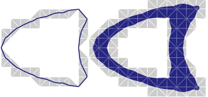
Figure 1.2.4: An example of the computational domains Γh and Dh for unfitted finite element methods.

whereσ(r)>0 if |r|< αω andσ(r) = 0 if|r| ≥αω for some constantαω>0.

In the phase field methodology, one often solves for an unknown interface (surface) represented by a phase field variable ϕ which has a step transition from

the bulk values≈ ±1 on either side of the interface. We can construct a phase field variable with compact support (i.e. the width of the interface is finite) with use of a

double obstacle phase field model (Blowey and Elliott 1991,1992). In this context,

we form a diffuse interface with

ρε=σ(ϕ), whereσ(r) = 1−r2.

In this approachϕ can be considered as a level set function for Γ.

Such a formulation was originally developed by Cahn, Fife and Penrose

(1997) for a complex moving boundary problem. Numerical methods were

pro-posed byDeckelnick, Elliott and Styles (2001) using a finite element method. The

approach was generalised to different equations in the work ofR¨atz and Voigt(2006) on stationary surfaces and extended to evolving surfaces by Elliott, Stinner, Styles

and Welford (2011). The formulation is based on an arbitrary triangulation of a

background region. To remain efficient, in practice, this is adaptively refined to resolve the interface. This approach has been used successfully to solve the

Cahn-Hilliard-Navier-Stokes system by Kay, Styles and Welford(2008).

To ensure the efficiency of level set methods, it has been suggested ( Deckel-nick, Dziuk, Elliott and Heine 2010; Olshanskii, Reusken and Grande 2009) to use

(24)

back-ground, fixed triangulation. The method has been successfully used for equations in

planar domains with curved boundaries using finite element methods (Barrett and Elliott 1982,1984, 1985,1987a,b,1988) and using discontinuous Galerkin methods

(Bastian and Engwer 2009;Engwer and Heimann 2012), as well as for an interface

problem (Hansbo and Hansbo 2002).

We describe these methods for a Poisson equation (1.1.1) on a surface Γ which is the zero level set of a smooth level set function Φ. This approach uses the

Eulerian formulation of surface partial differential equations. The work ofDeckelnick et al.(2010) considers an approximation of a surface Poisson equation using a bulk

finite element spaceVh defined over a union of elements which intersectDh :={x∈

Rn+1 :|Φh(x)|< ε}; seeFigure 1.2.4 for example. To ensure optimal order errors, the authors coupleε=βh, forβ >0, and solved:

Z

Dh

Ph∇uh· ∇φh|∇Φh|+uhφh|∇Φh|dx=

Z

Dh

feφh|∇Φh|dx, for allφh ∈Vh,

where Φh is a numerical approximation of Φ (for example, the nodal interpolant),

P_h element-wise projection given by

Ph(x) = Id−νh(x)⊗νh(x), νh(x) =

∇Φh(x)

|∇Φh(x)|

, forx∈Dh.

One may also consider the limit of these equations asβ→0 to derive a sharp interface approximation. We set Γh := {x ∈Rn+1 : Φh(x) = 0} (see Figure 1.2.4), and Vh is a bulk finite element space over elements which intersect Γh (plus some technical details). This is the method ofOlshanskii et al. (2009) who solve:

Z

Γh

∇_Γ_huh· ∇Γhφh+uhφhdσh=

Z

Γh

feφhdσh, for all φh∈Vh.

This finite element scheme is not initially well-posed unless we restrict the problem

to finite element functions with ∇φh·νh = 0 where νh is the element-wise normal to Γh. This does not cause any problems numerically since solutions can be

com-puted with the usual finite element basis functions used as a spanning set via the

conjugate gradient method. The induced triangulation, the underlying triangula-tion restricted to the computatriangula-tional domain, may have arbitrarily small elements,

hence the resulting system of linear equations may be extremely badly conditioned.

Analysis and numerical tests byOlshanskii and Reusken(2010) show that a simple Jacobi preconditioner overcomes this problem. Recent work byOlshanskii, Reusken

(25)

[image:25.595.222.423.107.245.2]

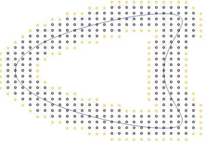
Figure 1.2.5: An example of the computational domain for the closest point method. The black nodes represent the nodes at which we calculate the solution of the partial differential equation. In addition the yellow nodes show the extra ghost nodes at which we must find the extended (interpolated) solution.

condition if the bulk triangulation satisfies a minimum angle condition.

An adaptive finite element method using the sharp interface approximation

has been studied by Demlow and Olshanskii (2012) and an advection dominated

problem is considered byOlshanskii, Reusken and Xu(2013). More details on these methods are given inChapter 4.

The final method we mention is the closest point method. The idea is to

cre-ate a very simple method by embedding a surface partial differential equation into a narrow band about the surface using the closest point operator (A.2.2) and then using Cartesian differential operators. The original method, proposed byRuuth and

Merriman(2008), proposes a two step method to construct solutions to (1.1.3) at each time step. First, one extends the solution off the surface to the computational

domain using the closest point operator, replacingu by u(p(·)). This step requires

computation of the closest point operator and nodal interpolation to find the so-lution away from nodal values. Then, one computes the soso-lution to the embedded

partial differential equation — the surface partial differential equation with

tangen-tial surface operators replaced with their Cartesian counterparts — using standard finite differences on a Cartesian mesh in the computational domain for one time

step. The computational domain is a narrow band about the surface defined by the nodes required to compute the finite difference stencil at each of the interpolation

nodes; see Figure 1.2.5 for example. In effect, the method approximates solutions to

(26)

The method relies on the fact that

∇u(p(x)) =∇_Γu(x) forx∈Γ.

This method has been generalised using different interpolation operators

(Macdonald and Ruuth 2008), using implicit time stepping (Macdonald and Ruuth

2009), and using more general closest point operators (M¨arz and Macdonald 2012). It has been applied to a wide variety of problems including eigenvalue problems on

surfaces (Macdonald, Brandman and Ruuth 2011). This method is incredibly cheap

and simple to use although it currently lacks rigorous analysis.

1.3 Applications of surface partial differential equations

Surface partial differential equations arise in a wide variety of applications. We give details of a few here as motivation for the methods that follow. Many more

applications have been studied. SeeDziuk and Elliott (2007b) for a more detailed

list.

Surface active agents

A strong motivating example for many of the methods listed above is that of

ad-vection and diffusion of a surface active agent (surfactant) on a fluid interface. Surfactants have an important role in many industrial and biological applications.

We mention in particular plastic production (Grace 1982), oil recovery (Morrow and

Mason 2001) and pulmonary function (Goerke 1998). Surfactants have the property of changing (normally reducing) the surface tension of the interface to which they

are bound.

We consider a situation with two immiscible viscous fluids, of equal densities, with a drop of one fluid inside another separated by an energetic interface. We

suppose that there is a surfactant which is insoluble in either of the fluids and hence

is confined to the interfacial region. We assume that the surface energy depends on the concentration of surfactant and thus leads to a concentration dependent surface

tension and the Marangoni effect.

We describe a model presented by Elliott et al. (2011). The mathematical formulation consists of a moving interface problem of Navier-Stokes form coupled to

an advection-diffusion equation on the interface. The problem is to find an interface

Γ(t) separating two fluid domains Ω1(t) and Ω2(t), a fluid velocity v, pressure p,

(27)

Navier-Stokes system:

∂tv+ (v· ∇)v=−∇p+ 1 Re∆v

∇ ·v= 0,

and on the unknown evolving surface Γ(t) we have mass and momentum balances:

[v]1₂ = 0 v·ν=VΓ

−pId + 2 ReD(v)

1

2

=− 1

Re Ca σ(u)H+∇Γσ(u)

.

Here ν is the unit normal vector field pointing into Ω1(t), H is the mean

curva-ture of Γ(t), σ(u) is the concentration dependent surface tension, Re and Ca are the Reynolds and capillary numbers (dimensionless numbers derived from physical

quantities), VΓ is the normal velocity of Γ(t) and D(v) = 1₂ ∇v+ (∇v)t

is a

de-formation tensor. Finally, [η]1₂ represents the jump of η between Ω1 and Ω2. The

concentrationu satisfies the conservation equation

∂•u+u∇_Γ·v− ∇_Γ·q= 0 on Γ(t),

whereq=q(u) is the flux by which uis driven.

Several numerical approaches have been taken to solve similar problems. We

mention the work ofXu, Li, Lowengrub and Zhao(2006),Lowengrub, Xu and Voigt

(2007), andXu, Yang and Lowengrub(2012) based on the level set method ofXu and

Zhao(2003); the authors of Ganesan and Tobiska(2009) andGanesan, Hahn, Held

and Tobiska (2012) used an Arbitrary Lagrangian-Eulerian surface finite element method; and Elliott et al. (2011) who took a phase field approach. The study of

James and Lowengrub(2004), who considered a conservative volume of fluid method,

and the work of Lai, Tseng and Huang (2008), who used the immersed boundary method ofPeskin (1972), pursue the same problem from a more physical point of

view.

In other situations, we may drop the assumption that the surfactant only exists on the interface between the two fluids (Defay and Prigogine 1966). In this

case, we will model soluble surfactants which may live on the interface Γ(t) or in

one of the bulk phases Ω2(t). Typically, we extend the previous model by assuming

(28)

satisfying:

∂tw+v· ∇w− ∇ ·qw = 0 in Ω2(t)

∂•u+u∇Γ·v− ∇Γ·qu =

∂w

∂ν on Γ(t),

wherequ andqw are the fluxes for the surfactant in Ω2(t) and Γ(t) respectively. The

system is completed by prescribing the flux of surfactant between bulk and interface phases:

∂w

∂ν +L(w, u) = 0,

or assuming instantaneous transport between the phases:

u=γ(w|_Γ(_t₎).

This model is similar to that derived by Bothe, Pr¨uss and Simonett (2005) and

Bothe and Pr¨uss(2010). The precise form ofLorγ will be determined by an adsorp-tion/desorption model governed by Langmuir kinetics. Modelling using Langmuir

kinetics can be found in work byNovak, Gao, Choi, Resasco, Schaff and Slepchenko

(2007); Kwon and Derby (2001); Booty and Siegel (2010); Medvedev and Stuche-brukhov(2011); andR¨atz and R¨oger (2012) in a variety of different applications.

Numerical methods have been derived for this extension, extending the

pre-vious works for insoluble surfactants. We mention in particular the work ofGarcke, Lam and Stinner(2013) and Teigen, Li, Lowengrub, Wang and Voigt (2009) both

using a phase field method. The review ofLi and Kim(2012) is also a useful

refer-ence.

Pattern formation on biological surfaces

The classical work ofTuring(1952) showed that many different patterns in nature

can be modelled by a simple system of reaction-diffusion equations. The review of Baker, Gaffney and Maini (2008) gives more modern biological applications of

what are now called Turing patterns. Numerical examples suggest that similar

reaction-diffusion systems posed on growing biological surfaces exhibit diffusion-driven instability of spatially uniform structures and thus lead to spatial patterns.

An example of such a model comes from the growth of solid tumours. The

evolution of the solid bulk tumour is determined by a concentration of growth pro-moting factor on the surface. The mathematical problem is to find the tumour

(29)

surface concentrations satisfying an evolution equation

V =−εH+δu,

and a system of reaction-diffusion equations

∂•u+u∇_Γ·v= ∆Γu+f1(u, w) ∂•w+w∇_Γ·v=Dw∆Γw+f2(u, w).

In the first equationεandδ are positive parameters. TheεH is a regularising term ensuring smoothness of the surface and theδureflects the promotion of growth of the

surface by the concentration ofu. In the reaction-diffusion system,Dwis the positive

diffusion coefficient of the species w and f1, f2 model the interactions between the

two surface concentrations. An example is the activator-depleted substrate model

(Schnakenberg 1979), known as the Brusselator model, in which

f1(u, w) =γ(a−u+u2w) and f2(u, w) =γ(b−u2w),

with γ, a, b > 0 constants. This model is a combination of ideas from the work of

Crampin, Gaffney and Maini(1999) and Chaplain, Ganesh and Graham(2001). Numerical studies of this model are given byBarreira, Elliott and

Madzva-muse(2011) using a surface finite element method and by Bergdorf, Sbalzarini and

Koumoutsakos (2010) using a Lagrangian particle method based on the level set methodology.

A similar model for brain growth was studied numerically by Lefevre and

Mangin (2010). Further numerical studies can be found in Varea, Aragón and Barrio(1999) andPlaza, Sánchez-Garduño, Padilla, Barrio and Maini(2004). Other

authors have considered problems where one of the chemical species may also live in

the interior bulk phase. For example,R¨atz and R¨oger(2012) consider a Turing-type model for Guanine-tri-phosphate (GTP) binding proteins in biological cells which

can exist in either cytosolic volume or membrane surface using ideas from Langmuir

kinetics similar to the models for soluble surfactants.

Both Neilson, Mackenzie, Webb and Insall (2011) and Elliott, Stinner and

Venkataraman (2012) consider problems in cell motility using a reaction-diffusion system called the Meinhardt model (Gierer and Meinhardt 1972). This is coupled

to a fourth order geometric equation for the cell membrane coming from a Helfrich

(30)

Phase separation on surfaces

The final example we consider comes from a model for the etching of silver in a

silver-gold alloy whose surface is immersed in an electrolyte. It is an example where

coupling surface evolution with a surface process leads to highly complex morphol-ogy. The following model was developed byErlebacher, Aziz, Karma, Dimitrov and

Sieradzki(2001) and Eilks and Elliott (2008).

The goal is to find a surface Γ(t), evolving with velocityv=V ν, representing a surface monolayer, and a surface concentration u, of gold atoms in the binary

mixture of gold and electrolyte adatoms in the surface monolayer, satisfying the

geometric law

V =−Jdiss=v0(1−δH),

and the conservation law

∂•u+u∇_Γ·v− ∇_Γ·q =V C0,

withC0 the bulk gold concentration andq the diffusive surface flux of adatoms given

by

q=−Jdiff =−b(u)∇Γw w=−γ∆Γu+ψ0(u),

wherew is the chemical potential, b(u) is a concentration dependent mobility and

ψis the double well free energy occurring in Cahn-Hilliard theory. The free energy

of regular solutionψis given by the logarithmic functional

ψ(u) = θcr

2 u(1−u) +

θ

4 ulogu+ (1−u) log(1−u)

. (1.3.1)

The parameterθrepresents the temperature of the system andθcr the critical

tem-perature. We assumeθ < θcrso thatψhas a double well form and phase separation

occurs. A typical form ofbisb(c) = B₂(1−u2). Computations based on the surface finite element method can be found inEilks and Elliott(2008).

Analysis of a surface finite element method for a Cahn-Hilliard equation on a

stationary surface is given byDu et al. (2011). Further computations can be found in Schoenborn and Desai (1999) and Marenduzzo and Orlandini (2013). Mercker,

Ptashnyk, K¨uhnle, Hartmann, Weiss and J¨ager (2012) considered a Cahn-Hilliard

type equation forced by terms depending on the curvature of the surface, again on a fixed surface.

Models of phase separation in biology have also been developed. Elliott et al.

(31)

studied a problem on biomembranes.

We conclude this section by summarising the challenges these particular applications

bring.

Curved surfaces: The underlying domain of the partial differential equations lives in curved space. Our numerical methods will have to find a way to capture the

essential geometric aspects of the surface. We wish to make no assumptions with respect to symmetry.

Evolving surfaces: The domains we consider may also be time dependent. The methods we design must have a way to track this change. Ideally, we wish

to try to use as many features of simpler systems as possible. This means we

wish to use a time stepping procedure that results in solving a sequence of problems each on a different stationary surface.

Large deformations: We wish to be able to make no restrictions on the size of the deformation of the surface. Large deformations and topology changes will

restrict the type of representation used for the surface.

Unknown evolutions: In most of the applications above the surface, and its evo-lution, is a priori unknown. This means we must combine our methods with

computational techniques which can determine the motion of the surface.

Bulk effects: The surface effects we are modelling may be physically coupled to systems living in a volume region about the surface. Our numerical methods

should be able to be combined with other methods for these equations.

Non-linear effects: The equations in this thesis are meant as model problems for the complicated systems presented above. As such, we should always have these applications in mind when making assumptions.

1.4 Outline of thesis

The original content of this thesis consists of three chapters. The first extends the

surface finite element method to problems where a diffusion on a surface is coupled to diffusion in a bulk domain. The second studies an evolving surface finite element

method applied to a Cahn-Hilliard equation. Finally, the third looks at new unfitted

(32)

The first problem we tackle, shown inChapter 2, is a coupled bulk-surface equation. Often, applications of the surface finite element method consider problems where the evolution of surface concentrations depend on ‘bulk effects’. These effects

fall into two broad categories. In each, we assume a surface is embedded in a

volumetric domain. In the first case, the substance which lives on the surface may also live in parts of the volumetric region. The second case considers an evolution

of the surface forced by some underlying equations for motion in the surrounding

volume. Of course, both effects can occur in the same model.

To develop a method for these applications, we consider the following model

problem. Given a domain Ω with closed boundary Γ, we seek a solution pairu: Ω→

Rand v: Γ→Rsatisfying

−∆u+u=f in Ω (1.4.1a)

(αu−βv) +∂u

∂ν = 0 on Γ (1.4.1b)

−∆Γv+v+ ∂u

∂ν =g on Γ. (1.4.1c)

We assume f: Ω → _R and g: Γ → _R are given functions and α, β are positive constants. Equations (1.4.1a) and (1.4.1c) represent diffusion equation in the bulk and on the surface, and (1.4.1b) represents the exchange of concentration between the bulk and surface phases. This particular choice of coupling on the surface has

been used by Novak et al. (2007). It can be viewed as a linearisation of the more

general equation

L(u, v) +∂u

∂ν = 0,

where∂uL(u, v)>0 and ∂vL(u, v)<0, which has been used by: Kwon and Derby

(2001); Booty and Siegel (2010); Medvedev and Stuchebrukhov (2011); and R¨atz and R¨oger (2012), for example. We leave the numerical analysis of more general

couplings, the parabolic case and evolving domains to future work.

Our method works by taking a polyhedral approximation Ωh of Ω and using the boundary faces of Ωh, which we will call Γh, as an approximation of Γ. We

then use a finite element method to solve a variational form of the above equations.

This work also includes the use of higher order isoparametric finite elements. We show well-posedness for these equations and derive optimal order error estimates

for the finite element method. This chapter also includes details of a numerical

implementation and examples to demonstrate the rates of convergence.

(33)

1958) can be used to model several natural phenomena; applications using a

Cahn-Hilliard equation can be found in Section 1.3. Analysis of the Cahn-Hilliard equa-tion, in planar domains, started in the 1980’s with the work ofElliott and Songmu

(1986) and numerical work of Elliott and French (1987, 1989) and Elliott, French

and Milner (1989), which was extended to stationary surfaces byDu et al. (2011). A review of the behaviour of the Cahn-Hilliard equation in the planar case is given

byElliott(1989).

We will study the following problem mathematically. We assume we are given an evolving surface{Γ(t)}, fort∈[0, T], with prescribed velocity v. We seek

a solutionu of

∂•u+u∇Γ·v= ∆Γ

−ε∆Γu+

1

εψ

0₍_u₎

on Γ(t), (1.4.2)

subject to the initial condition u(·,0) = u0 on Γ(0) = Γ0. This is a fourth-order

non-linear equation posed on an evolving domain. We will look for solutions via

a second-order splitting method. We assume that ε is a small, but fixed, positive

parameter andψis the quartic double-well potential given by

ψ(z) = 1 4(z

2₋₁₎2_.

This is taken as a simplification of the logarithmic potential (1.3.1). We note that for general surface evolutions the Ginzburg-Landau functional will not decrease along

solutions of this equation and (1.4.2) is not a gradient flow. One can enforce energy decrease by imposing extra assumptions on v. Alternatively, one can calculate a coupled gradient flow equation foruandvusing techniques fromElliott and Stinner

(2010a).

This chapter is broken into four sections. In the first we derive the continuous

equation above (1.4.2). This comes from a simple conservation law on a surface and applying a generalisation of the Reynolds transport theorem to curved surfaces. Next, we derive our evolving surface finite element method. This is based on the

original method ofDziuk and Elliott(2007a). In section four, the discrete solution is

shown to satisfy an energy bound, hence we can use weak convergence results, along with domain perturbation arguments, to show that the continuous equations have

a solution. The fifth section then shows that the finite element method converges

with optimal order errors in appropriate surface norms. The chapter finishes with various numerical examples confirming the analytical results.

(34)

a level set function describing the surface which may have been obtained using a

level set or phase field method for a geometric partial differential equation. This method has the possibility of use in a large variety of applications where volumetric

forces determine the position and geometry of an evolving interface. We would like a

method with the efficiency of the parametric approach of the surface finite element method, but without worrying about constructing a good triangulation from an

implicit representation of the surface. Our starting points are the sharp interface

method ofOlshanskii et al.(2009) and the narrow band method ofDeckelnick et al.

(2010). We extend these methods by using the full Cartesian gradient of basis

functions instead of projecting onto the tangential directions to the surface.

Given a smooth level set function Φ with Γ = {x ∈ Rn+1 : Φ(x) = 0}, we

wish to solve the surface elliptic problem:

−∆Γu+u=f on Γ. (1.4.3)

We assume we have a fixed bulk triangulation T_h of a neighbourhood of Γ and

Φh is some approximation of Φ (the nodal interpolant, for example). We define

Γh := {x ∈ Rn+1 : Φh(x) = 0} and Dh := {x ∈ Rn+1 : |Φh(x)| < h}, which both consist of partial elements. For the sharp interface method, we set Vh to be

the space of piecewise linear finite element functions over the set of elements inTh

which intersect Γh (plus some technical assumptions) and solve

Z

Γh

∇uh· ∇φh+uhφhdσh=

Z

Γh

feφhdσh for allφh ∈Vh. (1.4.4)

Alternatively, for the narrow band method, we setVh to be the space of piecewise

linear finite element functions over the set of elements in Th which intersects Dh

and solve

1 2h

Z

Dh

∇uh· ∇φh+uhφhdx= 1 2h

Z

Dh

feφhdx for allφh ∈Vh. (1.4.5)

The use of full gradients means we no longer have degenerate equations to

solve and gives us control over the error of our finite element method away from the surface since we can bound the gradient of the error in the normal direction to the

surface. The properties of these new methods are explored both analytically and

numerically for a surface Poisson equation (1.4.3) and are shown to give comparable results to the surface finite element method.

(35)

as proposed byDziuk (1988). Many of the proofs from main chapters are given in

full detail here taken from Dziuk and Elliott (2013b). This section also includes details of numerical experiments which will be used as a basis for comparison for

(36)

Chapter 2

A finite element analysis of a

coupled bulk-surface equation

2.1 Introduction

In this chapter, we will describe and analyse a method for solving equations arising

from models with both bulk and surface effects taken into account. The key idea is to take a polyhedral approximation of the bulk region, consisting of a union of

simplices, and to use its boundary faces as an approximation of the surface. Using

the boundary faces in our calculations allows us to use the surface finite element method, as described in Appendix A, to calculate and analyse the surface terms in our equations. The novelty of this work is to combine these ideas with previous

studies ofLenoir(1986),Bernardi(1989) andDubois(1990) to account for the errors coming from the bulk terms.

We will restrict the presentation to a sample linear elliptic problem. Given a

sufficiently smooth boundary, we will show error bounds of orderhkin theH1norm and orderhk+1 in theL2 norm, wherek is the polynomial degree of the underlying

finite element space andhis the mesh size. This coincides with both error estimates

for planar domains (for example,Brenner and Scott 2002) and elliptic equations on surfaces (Demlow 2009). This is because any errors introduced by the approximation

(37)

2.1.1 The coupled system

For a bounded domain Ω⊂_Rn _{with boundary Γ, we seek solutions} _u_{: Ω}_→

Rand v: Γ→_Rof the system

−∆u+u=f in Ω (2.1.1a)

(αu−βv) +∂u

∂ν = 0 on Γ (2.1.1b)

−∆Γv+v+ ∂u

∂ν =g on Γ. (2.1.1c)

Here we assume that f and g are known functions on Ω and Γ, respectively, and

α, β >0 are positive constants. We can think of α andβ as constants coming from

non-dimensionalising a physical model. We denote by ∆Γ the Laplace-Beltrami

operator on Γ and by ν the outward pointing unit normal to Γ.

2.1.2 Outline of chapter

The chapter proceeds as follows. In the second section we will derive a variational

form for the equations and explore existence, uniqueness and regularity of solutions. The third section focuses on how to construct our computational domain and the

errors this introduces into our method. In the fourth section we develop the finite

element method and in the fifth section we will look for error bounds for this method. In the final section we will show some numerical results.

Throughout, we will use the notation ofDeckelnick et al.(2005) introduced

inAppendix A.

2.2 Well-posedness of the continuous problem

In this section, we introduce the variational form that the method is based on. We go on to prove an existence and uniqueness result using the Lax-Milgram theorem

(Evans 1998) and then show a regularity result by considering the bulk and surface

equations separately. Throughout this chapter, we will make the same assumptions on the domain as inAppendix A, except now since Ω⊂_Rn_{, we assume that Γ is an} (n−1)-dimensional hypersurface.

2.2.1 Variational form

We take functions η: Ω → R and ξ: Γ → R in a suitable space of test functions,

(38)

Z

Ω

∇u· ∇η+uηdx−

Z

Γ η∂u

∂ν dσ= Z

Ω

f ηdx, (2.2.1a)

Z

Γ

∇_Γv· ∇_Γξ+vξdσ+

Z

Γ ∂u ∂νξdσ=

Z

Γ

gξdσ. (2.2.1b)

The boundary condition (2.1.1b) tells us that

−

Z

Γ η∂u

∂νdσ = Z

Γ

(αu−βv)ηdσ and

Z

Γ ∂u

∂νξdσ =− Z

Γ

(αu−βv)ξdσ. (2.2.2)

We substitute these into (2.2.1) to get

Z

Ω

∇u· ∇η+uηdx+

Z

Γ

(αu−βv)ηdσ=

Z

Ω

f ηdx, (2.2.3a)

Z

Γ

∇_Γv· ∇_Γξ+vξdσ−

Z

Γ

(αu−βv)ξdσ=

Z

Γ

gηdσ. (2.2.3b)

We now take a weighted sum of (2.2.3a) and (2.2.3b) to obtain the variational form

α Z

Ω

∇u· ∇η+uηdx+β Z

Γ

∇_Γv· ∇_Γξ+vξdσ

+

Z

Γ

(αu−βv)(αη−βξ) dσ=α Z

Ω

f ηdx+β Z

Γ gξdσ.

(2.2.4)

We will test this variational form over the space H1(Ω)×H1(Γ), which we

define to be the product space

H1(Ω)×H1(Γ) :={(η, ξ) :η∈H1(Ω) and ξ ∈H1(Γ)}.

We equip this space with the inner product

h(η1, ξ1),(η2, ξ2)iH1_(Ω)_×_H1_(Γ):=hη₁, η₂i_H1_(Ω)+hξ₁, ξ₂i_H1_(Γ),

and induced norm given by

k(η, ξ)k_H1_(Ω)_×_H1_(Γ):= kηk2_H1_(Ω)+kξk2_H1_(Γ) 1

2_.

It is clear that H1(Ω)×H1(Γ) is a Hilbert space with this inner product. Details

of how to define the surface Sobolev spaceH1(Γ), and higher order spaces, can be

found in Appendix A. Using a Sobolev space formulation requires us to interpret

(39)

Theorem 2.2.1 (Trace Theorem). Assume Ω is bounded and Γ = ∂Ω is C1 and

1≤p <∞. Then there exists a bounded linear operator

T:W1,p(Ω)→Lp(Γ) (2.2.5)

such that T w = w|_Γ if w ∈ W1,p(Ω)∩C( ¯Ω). Furthermore there exists a constant cT, depending only on p andΩ such that

kT wk_Lp_(Γ)≤cTkwkW1,p_(Ω), (2.2.6)

for each w∈W1,p(Ω). We callT w the trace of w onΓ.

Proof. A proof is given is by Evans(1998, Chapter 5.5, Theorem 1).

Throughout, we will writeu forT u on Γ.

We will approximate solutions of the weak from of (2.1.1): Find (u, v) ∈

H1(Ω)×H1(Γ) such that

α Z

Ω

∇u· ∇η+uηdx+β Z

Γ

∇_Γv· ∇_Γξ+vξdσ

+

Z

Γ

(αu−βv)(αη−βξ) dσ=α Z

Ω

f ηdx+β Z

Γ gξdσ

(2.2.7)

for all (η, ξ)∈H1(Ω)×H1(Γ).

To help with the notations later, we will writea (u, v),(η, ξ)for the left-hand side

of this equation and l (η, ξ) for the right-hand side. In this way, we can rewrite (2.2.7) as

a (u, v),(η, ξ)=l (η, ξ) for all (η, ξ)∈H1(Ω)×H1(Γ). (2.2.8)

2.2.2 Existence, uniqueness and regularity

(40)

To see thatais bounded, we notice that for (w, y),(η, ξ)∈H1(Ω)×H1(Γ),

a (w, y),(η, ξ)≤αkwk_H1_(Ω)kηk_H1_(Ω)+βkyk_H1_(Γ)kξk_H1_(Γ)

+

Z

Γ

(αw−βy)(αη−βξ) dσ

≤√2 max{α, β} k(w, y)k_H1_(Ω)_×_H1_(Γ)k(η, ξ)k_H1_(Ω)_×_H1_(Γ)

+ 2c2_T max{α, β}2k(w, y)k_H1_(Ω)_×_H1_(Γ)k(η, ξ)k_H1_(Ω)_×_H1_(Γ)

≤ck(w, y)k_H1_(Ω)_×_H1_(Γ)k(η, ξ)k_H1_(Ω)_×_H1_(Γ).

(2.2.9) Here cT is the constant from the Trace Theorem (Theorem 2.2.1). Coercivity of a is immediate since we have for (η, ξ)∈H1(Ω)×H1(Γ),

a (η, ξ),(η, ξ)=αkηk2_H1_(Ω)+βkξk2_H1_(Γ)+kαη−βξk2_L2_(Γ)

≥√2 min{α, β} k(η, ξ)k2_H1_(Ω)_×_H1_(Γ).

(2.2.10)

Henceais coercive on H1(Ω)×H1(Γ) as α, β >0.

It is clear that l is bounded under the assumption that f ∈ H−1(Ω) and

g∈H−1(Γ).

Theorem 2.2.2 (Existence and uniqueness). Given α, β > 0, f ∈ H−1(Ω) and g∈H−1(Γ) there exists a unique pair (u, v)∈H1(Ω)×H1(Γ) such that

a (u, v),(η, ξ)=l (η, ξ) for all(η, ξ)∈H1(Ω)×H1(Γ). (2.2.11)

Furthermore, if Γ isC3, we can achieve bounds in theH2-norm by considering

restricting the bilinear formaby setting η and ξ equal to zero in turn. Forη= 0, we get

β Z

Γ

∇_Γv· ∇_Γξ+vξdσ+β2 Z

Γ

vξdσ=β Z

Γ

gξ+αβ Z

Γ

uξdσ for all ξ ∈H1(Γ).

This is exactly the variational form of the equation

−β∆Γv+ (β+β2)v=βg+αβu on Γ.

By the Trace Theorem (Theorem 2.2.1) andTheorem 2.2.2, we know thatu∈L2(Γ). Hence by surface elliptic theory (Aubin 1982), similarly to Theorem A.2.5, we have thatv∈H2(Γ) and have the bound

kvk_H2_(Γ)≤c kgk_L2_(Γ)+kvk_L2_(Γ)+kuk_H1_(Ω)

(41)

Forξ= 0, we get

α Z

Ω

∇u· ∇η+uηdx+α2uηdσ =α Z

Ω

f ηdx+αβ Z

Γ

vηdσ for all η∈H1(Ω).

This equation arises as the variational form of the equation

−α∆u+αu=αf in Ω

∂u

∂ν +αu=βv on Γ.

By regularity theory of elliptic problems with Robin boundary data (see Ladyzhen-skaia and Uraltseva (1968) or Gilbarg and Trudinger (2001)), if Γ is C3, we have

thatu∈H2(Ω) with the bound

kuk_H2_(Ω) ≤c kfk_L2_(Ω)+kvk_H1/2_(Γ)

. (2.2.13)

Combining (2.2.12) and (2.2.13) gives the following regularity result:

Theorem 2.2.3 (Regularity). Let Γ be C3, f ∈L2(Ω), g∈L2(Γ) andα, β >0. If

(u, v) solves the variational problem (2.2.7) then(u, v)∈H2(Ω)×H2(Γ)and

k(u, v)k_H2_(Ω)_×_H2_(Γ)≤c kfk_L2_(Ω)+kgk_L2_(Ω)

. (2.2.14)

2.3 Domain perturbation

The first step we take in discretising the system (2.1.1) is to create a polyhedral domain ˇΩh with boundary ˇΓh and then describe higher order approximations Ω(_hk)

and Γ(_hk). Our finite element method will be based on these domains. In this section,

we will explain how to construct such a domain and provide estimates for the errors introduced by approximating the domain. To prove the results in this section, we

will assume Γ isCk+1.

2.3.1 Domain approximation

We follow ideas taken from the work ofLenoir(1986), Bernardi(1989) andDubois

(1990) in order to define the triangulation of our bulk domain and results of Dziuk

(1988),Dziuk and Elliott(2007a) and Demlow (2009) to make estimates about the perturbation of the boundary of this domain. The higher order surface finite element

(42)

[image:42.595.136.507.111.263.2]

Figure 2.3.1: An example of a triangulated domains ˇΩh in R3, cut open to see the

interior simplices. These have been created using the CGAL package’s 3D Mesh Generation demos. SeeAlliez et al.(2012) for details. These polyhedra are approx-imations of Ω ={x: Φ(x)<0} with Φ from (2.6.1)

.

Let ˇΩh be a polyhedral approximation of Ω and set ˇΓh:=∂Ωˇh. We suppose that the faces of ˇΓh are (N −1) simplices whose vertices lie on Γ so that ˇΓh is

a discrete approximation of Γ in the sense of Section A.3.1. We assume this is given at the start of the procedure; see for exampleFigure 2.3.1. We take a quasi-uniform triangulation Tˇh of ˇΩh (Definition A.3.1) consisting of closed simplices, either triangles inR2 or tetrahedra inR3.

We define h := max{diam(T) : T ∈ Tˇ_h} and assume that h is sufficiently small so that ˇΓh⊆U so that for allx∈Γˇh, there exists a unique pointp=p(x)∈Γ

defined by (A.2.2). Finally, we assume that for each T ∈Tˇ_h, T ∩Γˇh has at most one face ofT.

Exact triangulation

In order to define our computational domains, we first define an exact triangulation

of Ω. An exact triangulation is made up of ‘curved simplices’ which together cover

all of Ω exactly.

The unit referencen-simplex is defined to be the unit simplex with vertices

at (0, . . . ,0), (1,0, . . . ,0), (0,1,0, . . . ,0), . . . , (0, . . . ,0,1). For each simplexT ∈Tˇ_h,

we define an affine functionFT:Rn→Rn which maps the unit referencen-simplex

ˆ

T onto T (mapping the vertices of ˆT onto the vertices of T) which we write as