http://wrap.warwick.ac.uk
Original citation:Zafar, Ammar, Radaydeh, Redha M., Chen, Yunfei and Alouini, Mohamed-Slim. (2014) Power allocation strategies for fixed-gain half-duplex amplify-and-forward relaying in Nakagami-m fading. IEEE Transactions on Wireless Communications, Volume 13 (Number 1). pp. 159-173.
Permanent WRAP url:
http://wrap.warwick.ac.uk/60219
Copyright and reuse:
The Warwick Research Archive Portal (WRAP) makes this work by researchers of the University of Warwick available open access under the following conditions. Copyright © and all moral rights to the version of the paper presented here belong to the individual author(s) and/or other copyright owners. To the extent reasonable and practicable the material made available in WRAP has been checked for eligibility before being made available.
Copies of full items can be used for personal research or study, educational, or not-for profit purposes without prior permission or charge. Provided that the authors, title and full bibliographic details are credited, a hyperlink and/or URL is given for the original metadata page and the content is not changed in any way.
Publisher’s statement:
“© 2014 IEEE. Personal use of this material is permitted. Permission from IEEE must be obtained for all other uses, in any current or future media, including reprinting
/republishing this material for advertising or promotional purposes, creating new collective works, for resale or redistribution to servers or lists, or reuse of any copyrighted component of this work in other works.”
A note on versions:
The version presented here may differ from the published version or, version of record, if you wish to cite this item you are advised to consult the publisher’s version. Please see the ‘permanent WRAP url’ above for details on accessing the published version and note that access may require a subscription.
Power Allocation Strategies for Fixed-Gain
Half-Duplex Amplify-and-Forward Relaying in
Nakagami-
m
Fading
Ammar Zafar,
Student Member, IEEE
, Redha M. Radaydeh,
Senior Member, IEEE
,
Yunfei Chen,
Senior Member, IEEE
, and Mohamed-Slim Alouini,
Fellow, IEEE
Abstract
In this paper, we study power allocation strategies for a fixed-gain amplify-and-forward relay network employing multiple relays. We consider two optimization problems for the relay network: 1) maximizing the end-to-end signal-to-noise ratio (SNR) and 2) minimizing the total power consumption while maintaining the end-to-end SNR over a threshold value. We investigate these two problems for two relaying protocols of all-participate (AP) relaying and selective relaying and two cases of feedback to the relays, full and limited. We show that the SNR maximization problem is concave and that the power minimization problem is convex for all protocols and feedback cases considered. We obtain closed-form expressions for the two problems in the case of full feedback and solve the problems through convex programming for limited feedback. Numerical results show the benefit of having full feedback at the relays for both optimization problems. However, they also show that feedback overhead can be reduced by having only limited feedback to the relays with only a small degradation in performance.
Index Terms
Amplify-and-forward, energy-efficiency, fixed-gain, full feedback, half-duplex, limited feedback, Nakagami-m fading, optimal power allocation.
This work was funded by King Abdullah University of Science and Technology (KAUST).
A. Zafar and M.-S. Alouini are with the Computer, Electrical and Mathematical Sciences & Engineering (CEMSE) Division, King Abdullah University of Science and Technology (KAUST), Thuwal, Makkah Province, Saudi Arabia. 23955-6900 (E-mail: {ammar.zafar, slim.alouini}@kaust.edu.sa).
Y. Chen is with the School of Engineering, University of Warwick, Coventry, UK. CV4 7AL (E-mail: [email protected]).
I. INTRODUCTION
The classical three-terminal relay channel has been around since the 1960s when it was first introduced by Van Der Meulen [1], [2]. Cover and Gamal then characterized the capacity of a three-terminal relay channel where a relay assists a source node in communicating with a destination node [3]. Since then precious little work was carried out on relays until a decade ago. The rapid progress in wireless communications technology, the increasing popularity of tetherless connectivity and satisfying the high quality-of-service (QoS) requirements have rekindled interest in relays [4], [5]. Recent years have seen a dearth of work being carried out to study the performance of relay-assisted systems [6]–[13]. It has been shown that relays can provide spatial diversity [14]–[16], increase capacity [17]–[19], conserve power [20], [21] and enhance coverage [22]–[24].
Power is a precious resource. It was reported in [25] that information and communication technology (ICT) utilizes more than 3% of the total electrical energy consumed worldwide and this percentage is expected to increase with time. Furthermore, in wireless communications, vendors and operators are searching for energy-efficient algorithms and devices to cut down on energy and operating costs [26]. In addition, mobile devices need to conserve energy as they have limited battery. Therefore, it is of paramount importance to use the available power as efficiently as possible. In a cooperative relay network, this corresponds to allocating power efficiently among the source and relay nodes to improve performance. Moreover, it is also essential to reduce overhead in the system which comes from feedback to the relays in the form of CSI, transmit power and other information. This usually requires the controller 1 to feedback
information to each relay. This causes great overhead and consumes precious system resources such as bandwidth and time. Thus, it is crucial to come up with power allocation strategies which can work with limited feedback to the relay to minimize the overhead [27]. However, this reduced overhead comes at the cost of degradation in performance as there is less knowledge to work with and exploit. Therefore, there is a performance-overhead trade-off. It is important to have insight into this trade-off, so that optimal decisions can be taken to improve system performance under different scenarios.
Power allocation for cooperative network with a single fixed-gain AF relay was studied in [28]–[32]. In [28], the authors proposed power allocation schemes to maximize the sum and product of the average SNR of the source-destination and average SNR of the relay-destination link for a fixed gain relay-assisted
1
source-destination pair. Moreover, the schemes required only knowledge of the channel statistics. For the same model as in [28], [29] proposed optimal and near-optimal power allocation algorithms to maximize the end-to-end SNR under slowly varying channel conditions. In [30], power allocation to minimize an upper bound on the symbol error rate (SER) for M-ary phase shift keying (MPSK) was derived for a source communicating with destination through a single fixed-gain AF relay. It was shown in [30] that the power allocation method provided better performance when the relay was near the destination. References [31] and [32] proposed power allocation strategies to minimize the bit error rate (BER) of a communication system employing a single fixed-gain AF relay. In [31], an upper bound on the pairwise error probability (PEP) is minimized for Rayleigh fading channels by efficiently allocating power between the source and relay nodes for different transmission protocols. The authors in [32] expanded upon the work in [31] by using the same PEP bound as in [31] and considering BER minimization for two single relay scenarios 1) moving relay 2) access point relay. For the moving relay case, the links were modeled as cascaded Nakagami random variables and for the access point case, the links were modeled as Nakagami random variables. For both cases, the upper bound on the PEP could not be obtained in closed-form in general. Closed-form bounds were obtained in the high SNR regime for the case when the relay is very close to the destination. These bounds involved the hypergeometric U-function [33, Eq. 9.211.4] which is difficult to implement. Hence, [32] suggested to numerically solve the problem for a large number of SNRs and Nakagami parameters and store the results in a look up table to be used for practical purpose.
upper and lower bounds for the outage probability were derived for the high SNR regime for Rayleigh fading channels. Then power allocation was performed to minimize both bounds simultaneously. Again as the problem was too complex, only closed-form expressions for the relay powers were derived and the optimal source power had to be found using an exhaustive search.
In this work, we consider a source-destination pair which communicates with the help of m fixed-gain AF relays. In addition to the m dual-hop links, the source and destination are also connected through a direct link2. The relays are assumed to have only one antenna and work in half-duplex mode. To avoid interference, all the relays are assumed to operate on orthogonal channels3. Moreover, coherent
detection is assumed. Hence, the destination has CSI of all the links which are modeled as Nakagami-m
random variables with arbitrary Nakagami parameter. To overcome the difficulty of obtaining a closed-form solution or efficient algorithm to calculate the source and relay powers jointly as was the case in [35], a relay gain model is used which depends on neither the instantaneous source power nor the instantaneous source-relay channel. Different from [35], this allows us to to show that the joint optimization problem is convex for the source as well as the relay powers. For this system, we consider two relay participation schemes of AP relaying in which all the m relays forward the signal to the destination and selective relaying in which only the selected 4 relay forwards the signal received from the source to the destination.
For both schemes, we consider two optimization problems of optimal power allocation (OPA) and energy-efficiency. We refer to these as dual problems. OPA refers to the problem of allocating power to the source and the relays to maximize the end-to-end SNR under a total power constraint on the system. In the dual problem of energy-efficiency, the total power consumed is minimized while keeping the end-to-end SNR above a certain threshold. For both problems, as the destination has full CSI, the power allocation is performed at the destination and the power of each relay is then fed back to it5. In this work, two cases of feedback to the relays are considered
1) Full feedback: In this case, power allocation is performed for each set of channel realization and fed back to the relays and the source. Thus, this is the optimal scenario and serves as a benchmark for
2The results in this paper include the case of no direct link as a special scenario by replacing the fading gain of the source-destination
link with 0. 3
They can be orthogonal in time, frequency, space, or code.
4How selection takes place is discussed in Section III where we study selective relaying in detail.
5
practical schemes. However, the drawback of this case is the great overhead due to feedback for each set of channel realizations. Note that the solution to this case is the same as the case when power allocation is performed at the source and the relays and they each have full CSI6. It is shown that
all the problems for full feedback can be efficiently solved in closed-form, including closed-form expression for the source power which was not obtained in previous related works.
2) Limited feedback: In this case, power allocation is performed using only the channel statistics. Hence, now the destination only needs to feedback the powers once before system startup. This results in degradation of performance. However, it reduces the feedback overhead considerably which is an important issue for cooperative relaying systems [27], [31], [32], [34], [35] The solution in this instance is the same as that when power allocation is performed at relays with knowledge of only channel statistics. This problem is solved assuming Nakagami-m fading with arbitrary Nakagami parameter which is different from previous works, such as [34] and [35] considering multiple relays. Moreover, the exact average end-to-end SNR is used as the selection metric. The concavity and convexity of the maximizing SNR and minimizing total power consumption is first established. Hence, the problems are then solved using convex optimization techniques. In addition, if the destination prefers simplicity and cannot solve a m+ 1 dimension convex optimization problem, then an upper bound is used for the average end-to-end SNR for integer Nakagami parameter which leads to simple closed-form solutions.
We study the two dual optimization problems for the two relay participation schemes under both cases of feedback given above. In [36], we studied the two dual problems for a similar system AP setup7,
not selective relaying. Moreover, in [36], we assumed that power allocation was performed at the relays which had only partial CSI of the links, not at the destination with full CSI. Such a system gives similar results to the full feedback case for AP relaying considered here. Hence, for full feedback with AP relaying in this work, we only give the results and a perfunctory discussion without derivation. The interested reader is referred to [36] for more details. Thus, the contribution of this work are the novel power allocation strategies for the different optimization metrics (i.e. maximizing end-to-end SNR and minimizing total power consumption), amount of feedback (i.e. full and limited), Nakagami-mfading with
6
Such an assumption was made in [35] and [39].
7We made a slight mistake for the implementation of the energy-efficiency problem solution in [36] which makes the results presented in
arbitrary Nakagami parameter and relaying strategy (i.e AP and selective). These novel power allocation strategies not only optimize the relay powers but the source power as well. Furthermore, the power allocation strategies work on the exact performance metric, i.e. instantaneous end-to-end SNR and average end-to-end SNR, and not on bounds except in the case where the destination prefers simplicity.
As well, we choose the end-to-end SNR as the performance metric for the following reasons. For the case of full feedback, the end-to-end SNR is the optimal criteria from an outage probability and ergodic capacity point of view, and it has to be used. For the case of limited feedback, it is not the optimal criteria anymore and the outage probability and the ergodic capacity should be used to find the optimal solution instead. However, it is very difficult to obtain these two metrics in a form suitable for evaluation, if not impossible. Most of the existing works which consider power allocation for the minimization of outage probability use bounds for Rayleigh fading channels to provide suboptimal solutions in the high SNR regime often around 20 dB, while in practical systems, the SNR may lie in the range of 5-10 dB because it is intractable to find the closed-form expressions of outage and capacity, even bounds for Nakagami-m
on the end-to-end SNR, generally, maximizing the average end-to-end SNR increases the instantaneous SNR on average which in turns means better outage performance and ergodic capacity.
The remainder of the paper is organized as follows. In Section II, we consider AP relaying. Section III focuses on selective relaying. Numerical results are presented in Section IV. Finally, Section V summarizes the main results of the paper.
II. ALL-PARTICIPATESCHEME
A. System Model
Consider a cooperative system with a source node, a destination node, and m relays. Each relay is assumed to be equipped with only one antenna and operates in half-duplex mode. The source and the relays transmit on orthogonal channels. Without loss of generality, we assume time division multiple access (TDMA). The transmission takes place in two phases. In the first phase, the source broadcasts information to the relays and the destination. The signals at the ith relay and the destination are given by ysi =
√
Eshsis+nsi and ysd =
√
Eshsds+nsd, respectively, where Es is the source energy, s is the
transmitted signal with unit energy, hsi and hsd are the instantaneous channel gains from the source to
the ith relay and destination, respectively, modeled as independent Nakagami-m faded, nsi and nid are
the complex Gaussian noise with mean zero and variances σ2
si andσsd2 , respectively. In the second phase,
the relays, after amplification, forward the signal to the destination. The received signal at the destination from the ith relay isyid =
√
aiEsEihsihids+ni, where ai is theith relay gain, Ei is the ith relay energy,
hid is the instantaneous channel gain from the ith relay to the destination again modeled as Nakagami-m
faded, ni is the equivalent noise with ni ∼ CN(0, σi2), and σ2i = aiEi|hid|2σ2si+σid2. One can write the
m+ 1 received signals at the destination in matrix form
y=hs+n, (1)
where h = hqEs
σ2
sd
hsd
q
aiEsE1
aiE1|h1d|2σ2s1+σ12d
hs1h1d. . .
q
aiEtEm
aiEm|hmd|2σ2sm+σ2md
hsmhmd
iT
, n ∼ CN(0,I), and
y = h 1
σsdysd
1
σ1y1d. . .
1
σmymd
iT
. Throughout this paper, it is assumed that the destination has complete CSI of all the links. It is also assumed that all the links experience independent fading. Furthermore, the fading gain of each link changes independently from one time slot to the other.
B. Optimal Power Allocation
1) Full Feedback: In this subsection, we assume that the destination feeds back information to each relay and the source. Using (1), and assuming maximal-ratio-combining (MRC) at the destination, the end-to-end SNR of the system is given by
γ =Es m
X
i=0
αi− m
X
i=1
αiζi
aiEiβi+ζi
!
, (2)
where α0 = |hsd|2
σ2
sd
, αi =
|hsi|2
σ2
si , βi =
|hid|2
σ2
id
, and ζi = σ12
si. In this work, we consider a total power constraint
on the whole system and individual power constraints on all the nodes. Hence, the power allocation problem can be written as
max
Es,Ei
γ, subject to Es+
m
X
i=1
Ei ≤Etot, 0≤Es≤Esmax, 0≤Ei ≤Eimax. (3)
where Etot is the total power constraint on the whole system, Esmax is the peak power constraint at the
source, and Eimax is the peak power constraint on theith relay. In general, γ is not a concave function of the source and relay powers as its Hessian is not negative semi-definite. However, as we show in Appendix A, the objective function in (3) is concave given the constraints on the system. Hence, the optimization problem in (3) can be solved using the Lagrange dual method [42]. Moreover, as the constraints are affine, Slater’s condition [42] is satisfied, i.e. the duality gap between the primal and dual solutions is zero. Therefore, the solution obtained for the Lagrange dual problem is also the optimal solution of the problem in (3). Hence, solving the problem in (3) using the Lagrange dual method, with the help of [36], yields the solution
Es =
δPm
i=1
q
αiζi
aiβi
2
(Pm
i=0αi−δ)
2 Emax s 0 (4)
Ej =
Pm i=1 q
αiζi
aiβi
(Pm
i=0αi−δ)
s
αjζj
ajβj
− ζj
ajβj
Ejmax
0 , (5) where δ= m X i=0
αi− m
X
i=1
s
αiζi
aiβi
! v u u t
(Pm
i=0αi)
Etot+Pmj=1 aζj
jβj
. (6)
from the one obtained in [35]. From equations (4) and (5), one can conclude that the OPA follows a filling solution. Hence, power is allocated in an iterative manner. However, unlike traditional water-filling algorithm, here the closed-form solution may change in an iteration according to the results in the previous iteration due to the fact that source and relay powers have different closed-form solutions unlike in works where only relay power allocation is performed and a generalized closed-form of the relay powers is obtained. Thus, if the source power exceeds its peak constraint, the expression for the relay powers changes accordingly. Also, if a relay power and not the source power exceeds its peak constraint, only the constraints and optimization variables are updated. If in the result of the current iteration the source power, Es, satisfies its constraints and any relay power does not satisfy its individual constraint,
then the analytical solution to the problem remains the same, however, the optimization variables and the constraint changes in the next iteration. Therefore, in this case, the optimal solution in the next iteration is given by
Es =
δP
i∈X
q
αiζi
aiβi
2
P
i6∈Yαi−δ−Pi∈Z
αiζi
aiEmaxi βi+ζi
2 Emax s 0 (7)
Ej =
P
i∈X
q
αiζi
aiβi
qα
jζj
ajβj
X
i6∈Y
αi−δ−
X
i∈Z
αiζi
aiEimaxβi+ζi
− ζj
ajβj
Emax j 0 (8) and
δ =X
i6∈Y
αi−
X
i∈Z
αiζi
aiEimaxβi+ζi
− X
i∈X
s
αiζi
aiβi
! v u u u u u u u t X
i6∈Y
αi−
X
i∈Z
αiζi
aiEimaxβi+ζi
Etot−
X
i∈Z
Eimax+X
j∈X
ζj
ajβj
, (9)
where X, Y and Z represent the sets of powers which satisfy the individual constraints and are less than zero and greater than the peak individual constraint, respectively. Now, if the source power comes out to be greater than Emax
s in the current iteration, then it is set at Esmax. The updated optimal solution for the
relay powers in the next iteration now becomes
Ej =
s
Emax s αjζj
δajβj
− ζj
ajβj
!Ejmax
0
where the Lagrangian multiplier can be obtained as
δ=
Esmax
P
j∈X
q
αjζj
ajβj
2
Etot−Esmax−
X
i∈Z
Eimax+X
j∈X
ζj
ajβj
!2. (11)
2) Limited Feedback: In Section II-B1, it was assumed that the destination fed back the transmit powers to each relay and the source for each channel realization. However, this greatly increases the overhead. The destination has to inform all relays of the power allocation through dedicated feedback channels. This consumes a considerable amount of resources. Moreover, the reverse link between the destination and the relays might be poor and communication might not be possible8. Therefore, it is desirable to be able to
work with less feedback. Hence, destination calculates the powers using channel statistics and only feeds back the powers once before system startup . Thus, to perform power allocation, the end-to-end SNR needs to be averaged over all the links. As the channels are modeled as Nakagami-m distributed, αi and
βi are both Gamma random variables and their probability density functions are given by
fαi(x) =
1
Γ(kαi)¯γ
kαi αi
xkαi−1e− x
¯
γαi and fβ i(x) =
1
Γ(kβi)¯γ
kβi βi
xkβi−1e− x
¯
γβi x≥0, (12)
respectively, where kαi and kβi are the shape parameters of the links, γ¯αi and γ¯βi are the average SNRs
of the links, and Γ(.)is the Gamma function. As all the links are assumed to be independent, the average end-to-end SNR can be found by averaging (2) over the density functions in (12) giving
¯ γ = Z ∞ 0 . . . Z ∞ 0 Es m X i=0
xi− m
X
i=1
xiζi
aiEiyi+ζi
!
1
Γ(kα0)¯γ kα0 α0
xkα0−1e− x
¯
γα0×
m
Y
i=1
1
Γ(kαi)¯γ
kαi αi
xkiαi−1e−
xi
¯
γαi 1
Γ(kβi)¯γ
kβi βi
yikβi−1e−
yi
¯
γβi
!
dx0dx1. . . dxmdy1. . . dym.
(13)
This can be simplified to
¯
γ =Es m
X
i=0
kαiγ¯αi −Es
m
X
i=1
¯
kαiγαiζi
Γ(kβi)¯γ
kβi βi
Z ∞
0
1
aiEiyi +ζi
yikβi−1e−
yi
¯
γβidy
i (14)
8
Solving the above with the help of [33, Eq. (3.383.10)] gives the average end-to-end SNR as
¯
γ =Es m
X
i=0
kαiγ¯αi −Es
m
X
i=1
kαi¯γαiζ
kβi i
akiβiγ¯βkβi
i
1
Eikβi e
ζi aiEi¯γβ
iΓ
1−kβi,
ζi
aiEiγ¯βi
, (15)
whereΓ(., .)is the upper incomplete gamma function given byΓ(s, z) = R∞
z e
−tts−1dt[33, Eq. (8.350.2)].
The optimization problem is the same as in II-B1, however the objective function is now changed to γ¯
instead ofγ. We show thatγ¯is a concave function of the optimization parameters on the domain of interest in Appendix B. Thus, the optimization problem is concave. However, it is difficult to find closed-form expressions for the optimal solution due to the complexity of the objective function. Fortunately, as the problem is concave, we can utilize well-known algorithms for convex optimization. So, the interior point algorithm can be used to find the optimal solution [42]. For the special case of Rayleigh fading, ¯γ in (15) simplifies to
¯
γ =Es m
X
i=0
¯
γαi−Es
m
X
i=1
ζiγ¯αi
aiEi¯γβi
e
ζi aiEi¯γβ
iE1
ζi
aiEiγ¯βi
, (16)
where E1(.) is the exponential integral function of the first kind and is related to the exponential integral
function as E1(x) =−Ei(−x) [43].
One last remark is that (15) contains the upper incomplete Gamma function which can be complex to implement. Moreover, the optimization problem is a numerical one with m+ 1 dimensions. Therefore, it is possible that the destination, if it is a simple node, does not have the capability to perform such computations. Furthermore, if power allocation is performed at the relay and the relay nodes are simple, then in this scenario, the relays will have difficulty in solving the m+ 1 dimension problem. Hence, a simple suboptimal solution is required in such scenarios. Using [44, Eq. (6.5.9)], γ¯, for integer values of the Nakagami parameter, can be written as
¯
γ =Es m
X
i=0
kαiγ¯αi −Es
m
X
i=1
¯
kαiγαiζi
aiEiγ¯βi
e
ζi aiEi¯γβ
iEk βi
ζi
aiEiγ¯βi
. (17)
Now utilizing [44, Eq. (5.1.19)], an upper bound on ¯γ can be found as
¯
γ ≤Es m
X
i=0
kαi¯γαi−Es
m
X
i=1
kαiγ¯αiζi
aiEiγ¯βi(kβi−1) +ζi
. (18)
its closest integer and then the upper bound in (18) can be maximized which as we show now yields simple closed-form results. Note that (18) can be obtained from (2) by replacing αi by kαi¯γαi and βi
by γ¯βi(kβi −1). Hence, the closed-form solution to maximizing the upper bound in (18) can simply be
obtained from the closed-form solution derived in Section II-B1 by making the given substitutions.
C. Energy-Efficiency
In Section II-B, we considered the problem of maximizing the end-to-end SNR under individual and total power constraints. In this section, we study the problem of energy-efficiency. The objective is to minimize the total power consumed, Etot = Es +
Pm
i=1Ei, while keeping the instantaneous end-to-end
SNR above a threshold, γth, and ensuring the source and relay powers do not exceed their respective
individual constraints. Like Section II-B, we consider the two cases of full and limited feedback.
1) Full feedback: The optimization problem is given by
min
Es,Ei Etot, subject to γ ≥γ
th, 0≤E
s ≤Esmax, 0≤Ei ≤Eimax. (19)
Now, we need to show that the optimization problem in (19) is convex and hence, the optimal solution can be found. The objective function and the individual constraints are convex functions. So, it is only left to show that γ is concave, meaning γth −γ is convex, on the interested domain of the problem. Employing the same notation and procedure as in Appendix A, to prove concavity of γ, we need to show that D(x, y) = (f(x)−f(y))(g(x)−g(y))≤0. Iff(x)> f(y), theng(y)> g(x), to satisfy the constraint on γ and vice versa. Thus, D(x, y)<0 andγ is concave on the domain. Moreover, γ is a monotonically increasing function of Es and Eis, hence the optimal solution to (19) is achieved when γ = γth. As
the other two constraints are affine and the objective function is convex, Slater’s condition is satisfied. Therefore, the solution obtained using the Lagrange dual method will be optimal. Solving the problem (19) using the Lagrange dual method, with the help of [36], gives the optimal solution as
Es =
ρPm
j=1
qα
jζj
ajβj
2
(ρPm
i=0αi−1)2
Emax s
0
(20)
Ej =
ρPm i=1
q
αiζi
aiβi
(ρPm
i=0αi−1)
s
αjζj
ajβj
− ζj
ajβj
Eimax
0
where ρ = Pm j=1 q
αjζj
ajβj
Pm
i=0αi
p
γth +
1
Pm
i=0αi
. (22)
From (20) and (21), one can see that the solution again follows a water-filling algorithm described in Section II-B1. Hence, the power allocation process is repeated until all the powers satisfy the constraint. However, the optimal solution changes depending on the initial power allocation. There are two cases like for the problem of OPA: 1) Es lies between 0 ans Esmax, 2) Es is greater than Esmax. Considering case 1
first, the optimal power allocation is given by
Es =
ρP
j∈X
qα
jζj
ajβj
2
ρX
i6∈Y
αi−ρ
X
i∈Z
αiζi
aiEimaxβi+ζi
−1 !2 Emax s 0 (23)
Ej =
ρP
i∈X
q
αiζi
aiβi
q
αjζj
ajβj
ρX
i6∈Y
αi−ρ
X
i∈Z
αiζi
aiEimaxβi+ζi
−1
− ζj
ajβj
Emax i 0 (24) and ρ= s P
j∈X
r
αj ζj aj βj
2
γth + 1
P
i6∈Yαi−Pi∈Z
αiζi
aiEimaxβi+ζi
. (25)
In the second case, Es=Esmax and
Ej =
s
ραjζjEsmax
ajβj
− ζj
ajβj
!Emaxj
0 , (26) ρ= Emax s P
i∈X
q
αiζi
aiβi
2
Emax s
X
i6∈Y
αi−
X
i∈Z
αiζi
aiEimaxβi+ζi
!
−γth
!2. (27)
situation can arise in this instance where γ > γth due to the powers greater than their constraint being
treated first in the algorithm. Hence, there should be a check at the end of the algorithm and if γ > γth,
then the whole water-filling process is repeated, however, this time the powers which came out to be zero in the first run of the complete procedure are not included in the algorithm from the start9.
2) Limited feedback: Now, we consider the case of limited feedback. As was the case in Section II-B2, the end-to-end SNR now needs to be averaged over all the links. Therefore, in this instance, the energy-efficiency optimization problem is given by
min
Es,Ei Etot, subject to ¯γ ≥γ
th, 0≤E
s ≤Esmax, 0≤Ei ≤Eimax, (28)
where γ¯ is given by (15). Using Appendix B and a similar argument as that in Section II-C1, it can be shown that the the optimization problem, (28), is convex. Hence, the Lagrange multiplier and other convex optimization algorithms can be applied to solve the problem. However, due to the complexity of the problem, it is very difficult to obtain closed-form expressions for the optimal solution. Therefore, we use the interior-point algorithm as utilized in Section II-B2 to obtain the optimal solution. Also, similar to Section II-B2, for simple nodes, the upper bound on ¯γ can be used, the results of which can be obtained from the results in Section II-B2 by making the appropriate substitutions.
III. SELECTIONSCHEME
In Section II, AP relaying was considered. However, AP relaying requires additional complexity at the destination to combine the relays. Also, as the relays transmit on orthogonal channels, it consumes a huge amount of system resources and decreases throughput. To ameliorate these drawbacks of AP relaying, selective relaying has been proposed in which only the “best” relay is selected to forward the signal from the source to the destination. The selection criteria depends on the objective. For OPA, the relay which maximizes the end-to-end SNR after power allocation is selected. For energy-efficiency, the relay which minimizes the consumed energy while fulfilling the constraint on the end-to-end SNR is selected. If no relay fulfills the constraint on the end-to-end SNR, then the relay which achieves the maximum end-to-end SNR is selected.
9
An important point to note is that while selective relaying is a special case of AP relaying and the solutions can be obtained in the same manner as in the AP case, it is better to re-formulate the problem as it reduces the number of computations and hence, conserves time and resources. For example, for OPA with full feedback, the new formulation requires only to find one variable and then both powers can be obtained from this variable with a simple multiplication. If this problem was solved using the methodology for AP, then three variables, source power, relay power and the Lagrange multiplier would need to be calculated which requires more computations. The computation saving is not significant for one channel realization, but becomes significant for large channel realizations. For the OPA limited feedback case, the convex optimization problem is converted from a two-dimensional problem to a one-dimensional problem which can be solved more efficiently. Therefore, re-formulating the problems has its benefits.
A. Optimal Power Allocation
1) Full feedback: For selective relaying, noting that the power is now only divided between the source and one relay, one can re-formulate the end-to-end SNR in (2), in the case that the ith relay is selected to transmit, as
γi =ηiEtot
α0+αi−
αiζi
ai(1−ηi)Etotβi+ζi
i= 1,2, . . . , m, (29) where we have replaced Es = ηiEtot, Ei = (1−ηi)Etot and 0< ηi ≤ 1. Ignoring the individual power
constraints, the optimization problem becomes
max
ηi
ηiEtot
α0+αi−
αiζi
ai(1−ηi)Etotβi+ζi
i= 1,2, . . . , m. (30) The concavity of the objective function follows from the concavity of the problem for AP relaying. Taking the derivative of the objective function in (30) and equating it to zero yields the optimal solution
ηi = 1−
1
aiEtotβi
s
(aiEtotβi+ζi)αiζi
α0+αi
−ζi
, (31)
where αi and βi are the links associated with the ith relay. If ηi is found to be such that one of the
powers exceeds its individual constraints, then ηi is adjusted so that the power lies on its peak individual
case, both the source and the selected relay transmit at their individual constraints. The algorithm for power allocation for selective relaying is
• Calculate ηi for all the relays using (31). • Compute the resulting γi for each relay. • Select the relay which has the maximum γi.
2) Limited feedback: As was the case for AP relaying, in the case of limited feedback, the end-to-end SNR has to be averaged over the channels before power allocation is performed. Hence, now the relay which gives best performance on average is now selected. The optimization problem now, with the help of (15), is
max
ηi
(1−ηi)Etot kα0γ¯α0 +kα0¯γαi−
kαi¯γαiζ
kβi i
akβi
i γ¯ kβi βi
1
ηkβi
i E
kβi tot
e
ζi aiηiEtot¯γβ
iΓ
1−kβi,
ζi
aiηiEtotγ¯βi
!
(32) where now Es = (1−ηi)Etot, Ei = ηiEtot and 0 ≤ ηi < 1 due to ease of analysis. The concavity of
the problem follows directly from the concavity of the AP case. Taking the derivative of the objective function in (32) and equating it to zero gives
0 =−Etot kα0¯γα0 +kα0¯γαi −
kαi¯γαiζ
kβi i
akiβiEtotkβi¯γβkβi
i
1
ηikβi e
ζi aiηiEtot¯γβ
iΓ
1−kβi,
ζi
aiηiEtotγ¯βi
!
−
(1−ηi)
kαiγ¯αiζ
kβi i
akiβiEtotkβi−1γ¯βkβi
i
− ζi
aiEtotγ¯βi
1
ηikβj+2
Γ
1−kβi,
ζi
aiηiEtot¯γβi
e
ζi aiηiEtotγβ¯
i−
kβi
1
ηkiβi+1
Γ
1−kβi,
ζi
aiηiEtot¯γβi
e
ζi aiηiEtot¯γβ
i + ζ
−kβi+1
i
a−i kβi+1η2
iE
−kβi+1
tot γ¯
−kβi+1
βi
!
.
(33)
Equation (33) can be solved numerically using algorithms such as bisection, Newton’s method etc to yield the optimal value of ηi. Similar to the full feedback case, ηi is found for all the relays and then the relay
which maximizes the averaged end-to-end SNR is selected. For the special case of Rayleigh fading, ηi
can be obtained from
0 =−Etot
¯
γα0 + ¯γαi −
ζiγ¯αi
aiηiEtot¯γβi
e
ζi aiηiEtotγβ¯
iE1
ζi
aiηiEtotγ¯βi
−(1−η)ζi¯γαi
aiγ¯βi
−1 η2 i e ζi aiηiEtot¯γβ
iE1
ζi
aiηiEtotγ¯βi
+ 1 ηi 1 ηi
−E1
ζi
aiηiEtotγ¯βi
e
ζi aiηiEtotγβ¯
i ζi
aiηi2Etot¯γβi
.
(34)
For the case of simple nodes, then the solution can be obtained from replacing αi by kαiγ¯αi and βi by
¯
B. Energy-Efficiency
1) Full CSI: In the case of full CSI, the energy-efficiency problem for the ith selected relay is
min
Es,Ei Etot, subject to γi ≥γ th
, 0≤Es ≤Esmax, 0≤Ei ≤Eimax, (35)
where
γi =Es
α0+αi−
αiζi
aiEiβi+ζi
. (36)
The optimization problem, (35), is solved for all the relays and the relay which minimizes Etot while
fulfilling the constraint on γi is selected. If no relay fulfills the constraint on γi, then the relay which
maximizes γi is selected.
Ignoring the individual constraints and taking advantage of the fact that at the optimal solution γ =γth,
we can write
Es =
aiEiβiγth+ζiγth
α0ζi+aiEiα0βi+aiEiαiβi
. (37)
Thus, ignoring the individual constraints, (35) can be re-written as
min
Ei
aiEiβiγth+ζiγth
α0ζi+aiEiα0βi+aiEiαiβi
+Ei. (38)
Taking the derivative and equating it to 0 gives Ei as
Ei =
p
aiαiβiζiγth−α0ζi
aiβi(α0+αi)
. (39)
Substituting (39) in (37) yields
Es =
√
aiαiβiζi+ζiα0
γth
(α0+αi)
p
aiαiβiζiγth
. (40)
Incorporating the individual constraints gives the water-filling solution
Es=
√
aiαiβiζi+ζiα0
γth
(α0+αi)
p
aiαiβiζiγth
!Esmax
0
Ei =
p
aiαiβiζiγth−α0ζi
aiβi(α0+αi)
!Eimax
0
2) Limited feedback: In this case, the selection procedure and the optimization problem are the same as in Section III-B1, however the constraint on the end-to-end SNR changes to γ¯i ≥γth, where
¯
γi =Es kα0¯γα0 +kαiγ¯αi−
kαi¯γαiζ
kβi i
akiβiγ¯βkβi
i
1
Eikβi e
ζi aiEi¯γβ
iΓ
1−kβi,
ζi
aiEiγ¯βi
!
. (42)
Again exploiting the equality of the constraint on γ¯i, we obtain
Es=
γthEikβi
(kα0¯γα0 +kαiγ¯αi)E
kβi
i −
kαiγ¯αiζkβi i
akβi i γ¯
kβi βi
e
ζi aiEi¯γβ
iΓ
1−kβi,
ζi
aiEi¯γβi
. (43)
Therefore, the optimization problem becomes
min
Ei
γthEkβi
i
(kα0¯γα0 +kαiγ¯αi)E
kβi
i −
kαi¯γαiζkβi i
akβi i γ¯
kβi βi
e
ζi aiEiγβ¯
iΓ
1−kβi,
ζi
aiEi¯γβi
+Ei. (44)
Taking the derivative and equating to 0 gives
(kα0γ¯α0 +kαi¯γαi)E
kβi
i −
kαi¯γαiζ
kβi i
akiβiγ¯βkβi
i
e
ζi aiEi¯γβ
iΓ
1−kβi,
ζi
aiEi¯γβi
!2
−γ
thk
αikβi¯γαiζ
kβi i
akiβiγ¯βkβi
i
e
ζi aiEi¯γβ
i×
Γ
1−kβi,
ζi
aiEiγ¯βi
Eikβi−1+ γ
thk αiγ¯αiζi
aiEi2γ¯βi
−γ
thk αi¯γαiζ
kβi+1
i
akiβi+1γ¯βkβi+1
i
Γ
1−kβi,
ζi
aiEiγ¯βi
e
ζi aiEi¯γβ
iEkβi
−2
i = 0.
(45) The above equation can be solved through bisection search to yield the value ofEiwhich can be substituted
back into (43) to obtain Es. The maximum ofEs and Ei is checked and if it exceeds its peak constraint,
then it is set at it its peak constraint and the other power is obtained from the constraint. If no power exceeds its respective peak constraint, then the minimum power is checked and if it is below 0, it is set to zero and the other power is obtained from the constraint.
For Rayleigh fading, (46) simplifies to
(¯γα0 + ¯γαi)Ei−
¯
γαiζi
aiγ¯βi
e
ζi aiEi¯γβ
iE1
ζi
aiEi¯γβi
2
−γ
thγ¯ αiζi
ai¯γβi
e
ζi aiEi¯γβ
iE1
ζi
aiEiγ¯βi
+γ
th¯γ αiζi
aiEi2γ¯βi
− γ
th¯γ αiζi
aiEiγ¯βi
E1
ζi
aiEiγ¯βi
e
ζi aiEi¯γβ
i = 0.
(46)
−10 −5 0 5 10 15 10−3
10−2 10−1 100
γp (dB)
BER
UPA (AP)
UPA−limited feedback (Sel) Limited feedback (Sel) Limited feedback (AP) UPA−full feedback (Sel) Full feedback (Sel) Full feedback (AP)
(a)
−10 −5 0 5 10 15
10−4 10−3 10−2 10−1 100
γp (dB)
BER
UPA (AP)
UPA−limited feedback (Sel) Limited Feedback (Sel) Limited feedback (AP) UPA−full feedback (Sel) Full feedback (Sel) Full feedback (AP)
[image:20.612.66.539.60.263.2](b)
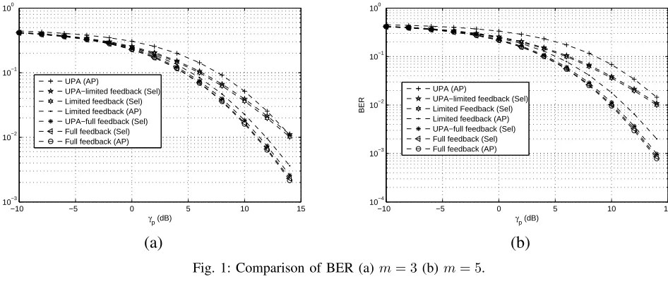
Fig. 1: Comparison of BER (a)m= 3(b) m= 5.
IV. NUMERICAL RESULTS ANDDISCUSSION
We present numerical results for the schemes discussed in this section. In the numerical results, all the noise variances are taken to be equal, i.e. σ2
sd = σsi2 = σ2id = σ2. The average SNR of all the links are
set at 0.5, i.e. γ¯αi = ¯γβi = 0.5, for i. All the shape parameters are taken to be 1 except when indicated
otherwise. The peak individual constraints are set as Emax
s = 3 and Eimax = 3 for all i. For OPA, Etot
is taken to be 5.5 and for energy-efficiency, γth is taken to be 10 dB. Also, for the energy-efficiency problem, it might be the case that due to channel conditions the constraint on the end-to-end SNR cannot be met. In that case all transmitting relays and the source transmit at their maximum power. The relay gain is modeled as ai = Emax 1
s kα0γ¯α0+σsi2 .
Figure 1 shows the comparison of the SER for the different schemes for BPSK as a function of
γp = Eσtot2 , which is a measure of the SNR, for m = 3 and m = 5. Firstly, we compare among the AP
and selection schemes for the different cases of CSI at the relays. It is evident from Figure 1 that the two OPA AP schemes comfortably provide better performance than uniform power allocation (UPA(AP)). Full feedback (AP) gives the greatest gain, as one would expect, of more than 4 dB and more than 3 dB for m = 5 and m = 3, respectively, over UPA (AP) at a BER of 10−2, while limited feedback (AP)
displays a gain of more than 2.5 dB and more than 2 dB for m= 5 and m= 3, respectively, at the same BER. Moreover, at a BER of 10−2, the performance difference between full feedback (AP) and limited
−100 −5 0 5 10 15 0.2
0.4 0.6 0.8 1 1.2 1.4 1.6 1.8
γp (dB)
Throughput (bits/sec/Hz)
Full feedback (Sel) UPA−full feedback (Sel) Limited Feedback (Sel) UPA−limited feedback (Sel) Full feedback (AP) Limited feedback (AP) UPA (AP)
(a)
−100 −5 0 5 10 15
0.2 0.4 0.6 0.8 1 1.2 1.4 1.6 1.8
γp (dB)
Throughput (bits/sec/Hz)
Full feedback (Sel) UPA−full feedback (Sel) Limited feedback (Sel) UPA−limited feedback (Sel) Full feedback (AP) Limited Feedback (AP) UPA (AP)
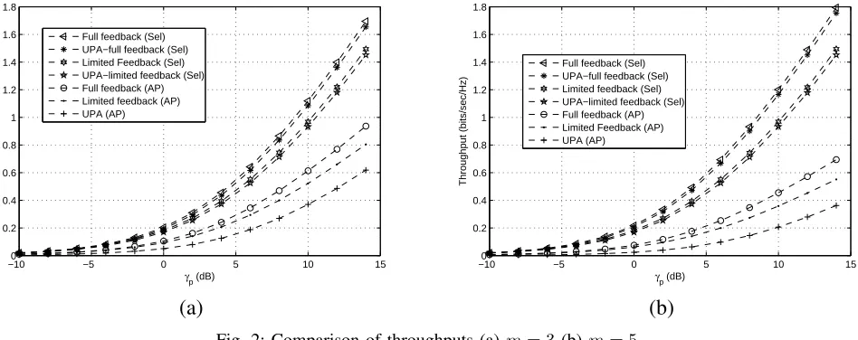
[image:21.612.69.543.62.250.2](b)
Fig. 2: Comparison of throughputs (a)m= 3 (b)m= 5.
relays which can be seen by comparing the increase in the performance gap between the two cases. Similar observations can be made for selective relaying. The two OPA schemes perform better than their UPA (Sel) counterparts for both cases of m = 3 and m = 5. However, the gain of full feedback (Sel) and limited feedback (Sel) over their UPA counterparts is small as compared to the AP case. But the gain of full feedback (Sel) over limited feedback (Sel) is quite large as compared to the AP case. Full feedback (Sel) outperforms limited feedback (Sel) by around 4 dB and 2.9 dB for m = 3 and m = 4, respectively. Thus, the decrease in performance due to limited feedback is severe in the case of selective relaying. Furthermore, full feedback (Sel) gives only a small degradation over full feedback (AP), while a large degradation is seen for the limited feedback scenario when moving from AP to selective relaying. An interesting point to note is that UPA (Sel) outperforms UPA (AP). This is due to the fact that even though AP has more relays, the total power is the same for both AP and selective relaying. For UPA (AP), this power is equally distributed among the relays and the source, however, for selective relaying the power is shared between only two nodes and moreover, the relay which maximizes the end-to-end SNR is selected. Thus, more power allocated to the relay which has better channel conditions and UPA (Sel) performs better than UPA (AP). However, as γp increases, all the relays see good channel conditions, in
general, and the gain of AP starts to manifest.
−100 −5 0 5 10 15 2
4 6 8 10 12 14
γs (dB) Etot
Full feedback (AP) Full feedback (Sel) Limited feedback (Sel) Limited feedback (AP)
(a)
−10 −5 0 5 10 15
10−3 10−2 10−1 100
γs (dB)
R
Limited feedback (Sel) Limited feedback (AP) Full feedback (Sel) Full feedback (AP)
[image:22.612.69.543.61.244.2](b)
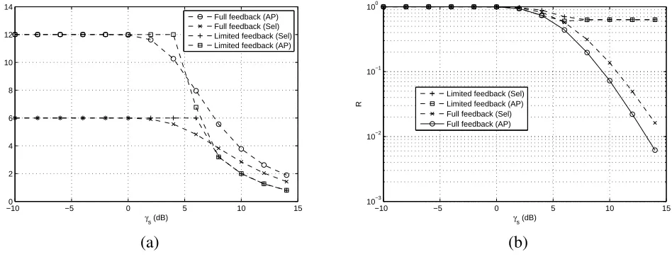
Fig. 3: Energy-efficiency form= 3(a)Etot (b)R.
in number of relays, while there is a decrease in throughput in the AP case. Furthermore, a similar pattern is observed for the throughputs as was seen for the SER case when comparing among the two relaying strategies, i.e full feedback achieves the best performance followed by limited feedback.
Jointly considering Figs. 1 and 2, it is clear that selective relaying is the preferred relaying strategy for the full feedback case. It provides the largest throughput and only leads to a small degradation in BER over full feedback (Sel). In addition, it requires less feedback then its AP counterpart, as in selective relaying only the selected relay needs to be informed of its power and no power feedback is required for the other relays. In the AP case, the power allocation is fed back to all the relays. In the case of limited feedback, the preference of relaying strategies depends upon the objective. If more robustness is required, then AP relaying should be performed. However, if higher data rates are required, then selective relaying seems to be the choice. Moreover, the from a feedback-performance trade-off point of view, there is a large gap in performance between the full feedback cases and limited feedback cases. However, the feedback is significantly reduced for limited feedback. Therefore, it depends mainly upon system specification which scheme to utilize. For example, if the quality of the feedback channels is quite poor on average, then feedback might not be possible in many scenarios. So, limited feedback can be utilized in this case.
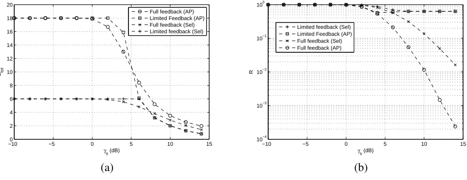
Figs. 3 and 4 show the results for the energy-efficiency problem for m = 3 and m = 5, respectively, as a function of γs = σ12, which is again a measure of the SNR. Except for some minor differences,
−100 −5 0 5 10 15 2
4 6 8 10 12 14 16 18 20
γs (dB) Etot
Full feedback (AP) Limited Feedback (AP) Full feedback (Sel) Limited feedback (Sel)
(a)
−10 −5 0 5 10 15
10−4 10−3 10−2 10−1 100
γs (dB)
R
Limited feedback (Sel) Limited Feedback (AP) Full feedback (Sel) Full feedback (AP)
[image:23.612.65.543.61.245.2](b)
Fig. 4: Energy-efficiency form= 5(a)Etot (b)R.
of the SNR, the system cannot achieve the minimum threshold on the end-to-end SNR for most channel realizations, hence, for AP relaying all the relays and the source transmit at their peak powers and for the selective relaying the source and the selected relay transmit at their peak powers. Thus in Fig. 3(a), the AP schemes transmit at 12 and the selection schemes transmit at 6 at low values of γs. Same in Fig. 4(a)
−100 −5 0 5 10 15 0.2
0.4 0.6 0.8 1 1.2 1.4 1.6 1.8
γp (dB)
Throughput (bits/sec/Hz)
Bound (AP) Limited Feedback (AP)
k=6 k=10
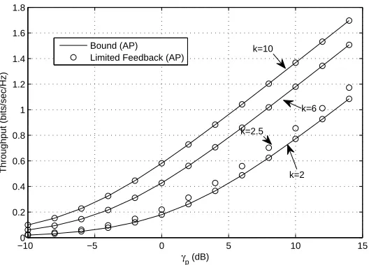
[image:24.612.172.436.63.253.2]k=2 k=2.5
Fig. 5: Effect of bounding the SNR form= 3andkαi=kβi=k.
They meet the end-to-end SNR constraint on average, however, don’t fulfill it instantaneously. Therefore, they don’t transmit at peak power even when the instantaneous SNR is below the constraint while the full feedback schemes transmit at peak powers and hence, consume more energy on average.
From Figs. 3 and 4, it can be concluded that, at low SNR, limited feedback (Sel) is the best scheme in terms of energy-efficiency and complexity. It achieves the same performance on average as the other schemes and requires less feedback and complexity. From medium SNR and onwards, full feedback (AP) is the best scheme. Even though it consumes more power, it achieves the constraint on the end-to-end SNR more frequently. This is particularly true for a system with large number of relays.
Fig. 5 shows the effect of bounding the the average end-to-end SNR10. It can be seen from Fig. 5 that for integer values of the Nakagami parameter, bounding the SNR has almost no effect. The upper bound on the average end-to-end SNR and the actual average end-to-end SNR give the same performance for all three values of the Nakagami parameter. Thus, for integer values, instead of using convex numerical optimization techniques, the closed-form expressions for the upper bound can be utilized without loss of performance. For the case of non-integer Nakagami parameter, the non-integer is first rounded down to the nearest integer less than the actual value. In this case, the bound gives the same performance as the actual one at low SNR. However, the gap in performance starts to grow with increase in SNR as can be seen from Fig. 5 for k = 2 and k = 2.5.
Fig. 6 shows the power allocation for both the considered problems for all scenarios. Fig. 6 (a) shows
0 0.1 0.2 0.3 0.4 0.5 0.6 0.7 0.8 0.9 0
0.5 1 1.5 2 2.5 3
Average SNR of the direct link
Power Allocation
Source Power (Full feedback −AP) Second Relay Power (Full feedback −AP) First Relay Power (Full feedback −AP) Source Power (Limited feedback −AP) Second Relay Power (Limited feedback −AP) First Relay Power (Limited feedback −AP) Source Power (Full feedback −Sel) Relay Power (Full feedback −Sel) Source Power (Limited feedback −Sel) Relay Power (Limited feedback −Sel)
(a)
0 0.1 0.2 0.3 0.4 0.5 0.6 0.7 0.8 0.9 1
1.2 1.4 1.6 1.8 2 2.2 2.4 2.6 2.8 3
Average SNR of the direct link
Power Allocation
Source Power (Full feedback −AP) Second Relay Power (Full feedback −AP) First Relay Power (Full feedback −AP) Source Power (Limited feedback −AP) Second Relay Power (Limited feedback −AP) First Relay Power (Limited feedback −AP) Source Power (Full feedback −Sel) Relay Power (Full feedback −Sel) Source Power (Limited feedback −Sel) Relay Power (Limited feedback −Sel)
[image:25.612.67.557.61.269.2](b)
Fig. 6: Power Allocation for (a) Energy-efficiency (b) optimal power allocation as function of the average SNR of the direct link with m= 2 and the average SNRs of the first relay are set as 0.8 and 1 for the two hops, respectively and the average SNRs of the second relay are set as 1 and 0.8.
the power allocation for the energy-efficiency problem with γs = 5 dB. Fig. 6 (a) clearly shows that, as
expected, the source power is the most important and is the highest for all the cases for all the values of the average SNR of the direct link. Furthermore, it can also be observed that the allocated source power decreases with better direct link. One interesting observation from Fig. 6 (a) is that, for the AP system, more power is allocated to the relay which has the better first hop when the direct link is of low quality and more power is allocated to the link which has the better second hop when the direct link has better quality11. The reason for this can be observed from equations (27) and (28) that the first term in (27) is a
decreasing function of the direct link and an increasing function of the first hop. Hence, when the direct link is low, this term dominated. However, when the direct link becomes better, the second term which is an increasing function of the second hop starts to have more influence. A similar behaviour is shown in Fig. 6 (b) for the problem of optimal power allocation to maximize the end-to-end SNR with γp = 5 dB.
However, in Fig. 6 (b), the source power increases with increase in the strength of the direct link due to more allocated to the link which has better channel conditions to maximize the end-to-end SNR12.
11This is more noticeable for the limited feedback case. For the full feedback case, as the values are very close, it is not exactly clear
from the plot.
12For further discussion on power allocation for both the problems, the interested reader is referred to [45] which is an extended version
V. CONCLUSIONS
We have studied power allocation to maximize the end-to-end SNR under a total power constraint and to minimize the the total power consumed while maintaining the end-to-end SNR above a required threshold for a fixed-gain AF relay network. We have studied both problems for the relay network operating in AP mode where all the relays participate in signal forwarding and operating in selection mode in which only the selected relay forwards the signal to the destination. Furthermore, we have also considered the cases of full feedback and limited feedback for both modes of operation and for both optimization problems. We demonstrated the convexity/concavity of all the problems. Moreover, for the full feedback case, closed-form expressions have been obtained for all the problems. For the limited feedback case, the optimization problems have been solved using convex programming. To alleviate the complexity of convex programming, we have utilized an upper bound on the average end-to-end SNR to obtain closed-form expressions for the limited feedback case too which give the same performance as the convex programming at integer Nakagami parameter. Furthermore, we demonstrate the gain achieved by allocating power optimally over UPA. We also give insight into the performance of the system for both problems, for both AP relaying and selective relaying and for the two cases of feedback. Additionally, we also develop inequalities in Appendix B which may prove to be useful in future works. Thus, we believe that our work is a valuable contribution to the already available literature on power allocation strategies for fixed-gain AF relays.
APPENDIXA
Writing down the objective function
γ =Es m
X
i=0
αi− m
X
i=1
αiζi
aiEiβi+ζi
!
. (47)
The objective function, in general, not convex and concave. However, as we show below, it is concave (its negative is convex) for the domain we are interested in.
Define vector E as
Now let us define
f(E) = [1 0 0. . .0]E=Es g(E) = m
X
i=0
αi− m
X
i=1
αiζi
aiEiβi+ζi
. (49)
Both f and g are positive and increasing on their domain. For f to be concave
f(θx+ (1−θ)y)≥θf(x) + (1−θ)f(y), (50)
where 0≤θ ≤1. The left hand side (LHS) in the above isθx1+ (1−θ)y1 and the right hand side (RHS)
is equal to θx1+ (1−θ)y1. As the LHS is equal to the RHS, f is concave. To show that g is concave,
forming the Hessian
Hg =
0 0 0 · · · 0
0 − Esα1ζ1a21β12
(a1E1β1+ζ1)3 0 · · · 0
0 0 − Esα2ζ2a22β22
(a2E2β2+ζ2)3 0 · · · 0
..
. ... . .. . .. ... ... ..
. ... . .. . .. ... ...
0 0 · · · − Esαmζma2mβm2
(amEmβm+ζm)3
. (51)
As the eigenvalues of Hg are non-negative,Hg is negative semi-definite, and hence g is concave. Now let
us define
h(E) =f(E)g(E) =Es m
X
i=0
αi− m
X
i=1
αiζi
aiEiβi+ζi
!
. (52)
For h to be concave (−h to be convex)
h(θx+ (1−θ)y)≥θh(x) + (1−θ)h(y). (53)
Therefore for concavity we have to show
∆≤0, (54)
where
As f and g are both positive and concave
(f g)(θx+ (1−θ)y)≥(θf(x) + (1−θ)f(y))(θg(x) + (1−θ)g(y)) (56) Substituting (56) in the expression of ∆ one has
∆≤θf(x)g(x) + (1−θ)f(y)g(y)−θ2f(x)g(x)−(1−θ)2f(y)g(y)
−θ(1−θ)f(x)g(y)−θ(1−θ)f(y)g(x).
(57) After some manipulation
∆≤θ(1−θ)D(x, y), (58)
where D(x, y) = (f(x)−f(y))(g(x)−g(y)). If D(x, y) ≤ 0, then the proof of concavity is complete. For optimal power allocation, if f(x) > f(y) then P
i∈yEi >
P
i∈xEi from the total power constraint.
Therefore, with power allocation, g(y) > g(x), as it g(.) is a concave functions of the relay powers, implying D(x, y)<0 and hence, concavity. Similarly, if g(x)> g(y), then power allocation means that
P
i∈xEi >
P
i∈yEi, which in turns means f(y)> f(x). Thus, D(x, y)<0 and the objective function is
concave.
APPENDIX B Recall
¯
γ =Es m
X
i=0
kαiγ¯αi −Es
m
X
i=1
¯
kαiγαiζi
Γ(kβi)¯γ
kβi βi
Z ∞
0
1
aiEiyi +ζi
yikβi−1e−
yi
¯
γβidy
i (59)
It is obvious that (59) is a concave function of Es. To check concavity with respect to Ej, let
ν(Ej) =
Z ∞
0
1
ajEjyj +ζj
yjkβj−1e−
yj
¯
γβj
dyj =
Z ∞
0
Pyj(Ej)Q(yj)dyj, (60)
where
Pyj(Ej) =
1
ajEjyj+ζj
Q(yj) = y
kβj−1
j e
−¯yj
γβj
. (61)
Therefore, to show thatγ¯is concave with respect toEj, one has to show thatν(Ej)is convex with respect
to Ej. It is straightforward to see that Pyj(Ej) is a convex and monotonically decreasing function of Ej
can be written
ν(θEj1+(1−θ)Ej2) =
Z ∞
0
Pyj(θE
1
j+(1−θ)E
2
j)Q(yj)dyj ≤
Z ∞
0
θPyj(E
1
j) + (1−θ)Pyj(E
2
j)
Q(yj)dyj.
(62) Hence
ν(θEj1+ (1−θ)Ej2)≤θν(Ej1) + (1−θ)ν(Ej2) (63)
and the proof of convexity is complete. Therefore, γ¯ is a concave function ofEj. The concavity of γ¯ also
implies from the second derivative condition
S(v, kβj)≥0 v >0, kβj >0, (64)
where v = ζj
ajEj¯γβj and
S(v, kβj) =−(2 +kβj)v
−kβj+1
−v−kβj+2+ Γ 1−k
βj, v
evv2+ 2kβjv + 2v+k
2
βj +kβj
. (65) Now using a similar argument as in Appendix A, the joint concavity of ¯γ can be established.
For the special case of Rayleigh fading, the proof of concavity establishes the relationship
E1(v)ev v2+ 2 + 4v
−v−3>0 v >0. (66) REFERENCES
[1] E. C. V. D. Meulen, “Transmission of information in a T-terminal discrete memoryless channel,” Ph.D. dissertation, University of
California, Berkeley, CA, 1968.
[2] ——, “Three-terminal communication channels,”Advances in Applied Probability, vol. 3, pp. 120–154, 1971.
[3] T. Cover and A. E. L. Gamal, “Capacity theorems for the relay channel,”IEEE Trans. Inf. Theory, vol. 25, no. 5, pp. 572–584, Sep.
1979.
[4] A. Sendonaris, E. Erkip, and B. Aazhang, “User cooperation diversity-Part I: System description,” IEEE Trans. Commun., vol. 51,
no. 11, pp. 1927–1938, Nov. 2003.
[5] ——, “User cooperation diversity-Part II: Implementation aspects and performance analysis,”IEEE Trans. Commun., vol. 51, no. 11,
pp. 1939–1948, Nov. 2003.
[6] J. N. Laneman and G. W. Wornell, “Distributed space-time-coded protocols for exploiting cooperative diversity in wireless networks,”
IEEE Trans. Inf. Theory, vol. 49, no. 10, pp. 2415–2425, Oct. 2003.
[7] M. O. Hasna and M.-S. Alouini, “End-to-end performance of transmission systems with relays over rayleigh-fading channels,”IEEE
[8] ——, “Harmonic mean and end-to-end performance of transmission systems with relays,” IEEE Trans. Commun., vol. 52, no. 1, pp.
130–135, Jan. 2004.
[9] P. A. Anghel and M. Kaveh, “Exact symbol error probability of a cooperative network in a Rayleigh-fading environment,”IEEE Trans.
Wireless Commun., vol. 3, no. 5, pp. 1416–1421, May 2004.
[10] M. O. Hasna and M.-S. Alouini, “A performance study of dual-hop transmissions with fixed gain relays,” IEEE Trans. Wireless
Commun., vol. 3, no. 6, pp. 1963–1968, Nov. 2004.
[11] H. Shin and J. Song, “MRC analysis of cooperative diversity with fixed-gain relays in Nakagami-m fading channels,” IEEE Trans.
Wireless Commun., vol. 7, no. 6, pp. 2069–2074, Jun. 2008.
[12] M. Di Renzo, F. Graziosi, and F. Santucci, “A comprehensive framework for performance analysis of dual-hop cooperative wireless
systems with fixed-gain relays over generalized fading channels,”IEEE Trans. Wireless Commun., vol. 8, no. 10, pp. 5060–5074, Oct.
2009.
[13] D. Senaratne and C. Tellambura, “Unified exact performance analysis of two-hop amplify-and-forward relaying in Nakagami fading,”
IEEE Trans. Veh. Tech., vol. 59, no. 3, pp. 1529–1534, Mar. 2010.
[14] J. Laneman, D. Tse, and G. Wornell, “Cooperative diversity in wireless networks: Efficient protocols and outage behavior,”IEEE Trans.
Inf. Theory, vol. 50, no. 12, pp. 3062–3080, Dec. 2004.
[15] Y. Jing and H. Jafarkhani, “Single and multiple relay selection schemes and their achievable diversity orders,”IEEE Trans. Wireless
Commun., vol. 8, no. 3, pp. 1414–1423, Mar. 2009.
[16] M. Elkashlan, P. L. Yeoh, R. H. Y. Louie, and I. B. Collings, “On the exact and asymptotic SER of receive diversity with multiple
amplify-and-forward relays,”IEEE Trans. Veh. Tech., vol. 59, no. 9, pp. 4602–4608, Nov. 2010.
[17] R. Pabst, B. Walke, D. Schultz, P. Herhold, H. Yanikomeroglu, S. Mukherjee, H. Viswanathan, M. Lott, W. Zirwas, M. Dohler,
H. Aghvami, D. Falconer, and G. Fettweis, “Relay-based deployment concepts for wireless and mobile broadband radio,” IEEE
Commun. Mag., vol. 42, no. 9, pp. 80–89, Sep. 2004.
[18] G. Kramer, M. Gastpar, and P. Gupta, “Cooperative strategies and capacity theorems for relay networks,” IEEE Trans. Inf. Theory,
vol. 51, no. 9, pp. 3037–3063, Sep. 2005.
[19] M. Shaqfeh and H. Alnuweiri, “Joint power and resource allocation for block-fading relay-assisted broadcast channels,” IEEE Trans.
Wireless Commun., vol. 10, no. 6, pp. 1904–1913, Jun. 2011.
[20] S. Cui, A. J. Goldsmith, and A. Bahai, “Energy-efficiency of MIMO and cooperative MIMO techniques in sensor networks,”IEEE J.
Sel Areas. Commun., vol. 22, no. 6, pp. 1089–1098, Aug. 2004.
[21] Z. Zhou, S. Zhou, J.-H. Cui, and S. Cui, “Energy-efficient cooperative communication based on power control and selective single-relay
in wireless sensor networks,”IEEE Trans. Wireless Commun., vol. 7, no. 8, pp. 3066–3078, Aug. 2008.
[22] H. Hu, H. Yanikomeroglu, D. D. Falconer, and S. Periyalwar, “Range extension without capacity penalty in cellular networks with
digital fixed relays,” inProc. IEEE Global Commun. Conf. (GLOBECOM’2004), Dallas, TX, Nov-Dec, 2004, pp. 3053–3057.
[23] Y. Yang, H. Hu, J. Xu, and G. Mao, “Relay technologies for WiMAX and LTE-Advanced mobile systems,” IEEE Commun. Mag.,
vol. 47, no. 10, pp. 100–105, Oct. 2009.
[24] H. Ekstrom, A. Furuskar, J. Karlsson, M. Meyer, S. Parkvall, J. Torsner, and M. Wahlqvist, “Technical solutions for the 3G long-term
evolution,”IEEE Commun. Mag., vol. 44, no. 3, pp. 38–45, Mar. 2006.