Low frequency strip waveguide array for flow measurement in hostile environments

(1)

University of Warwick institutional repository:

http://go.warwick.ac.uk/wrap

A Thesis Submitted for the Degree of PhD at the University of Warwick

http://go.warwick.ac.uk/wrap/77475

This thesis is made available online and is protected by original copyright.

Please scroll down to view the document itself.

(2)

Low Frequency Strip Waveguide Array for Flow

Measurement in Hostile Environments

by

Michael Richard Laws

Thesis

Submitted to the University of Warwick

for the degree of

Doctor of Philosophy

Physics

(3)

List of Figures

2.1 A schematic diagram of a classical orifice meter. . . 9

2.2 A schematic diagram of a classical Venturi meter. . . 10

2.3 A schematic diagram of a classical turbine meter. . . 11

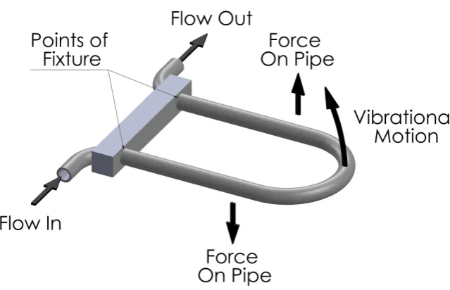
2.4 A schematic diagram of a U-shaped coriolis meter. . . 13

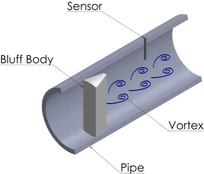
2.5 A schematic diagram of a vortex-shedding meter. . . 14

2.6 A schematic diagram of a electromagnetic meter. . . 15

2.7 A schematic diagram of a ITMF meter. . . 17

2.8 A schematic diagram of an ultrasonic Doppler meter. . . 18

2.9 A schematic diagram of an ultrasonic transit time meter. . . 20

(8)

3.2 The thickness resonances of a piezoelectric crystal demonstrated as a superposition of waves. The two edges of the PZT oscillate symmetri-cally about the centre of the element, with the yellow wave travelling to the left and the black wave travelling to the right. When the thick-ness of the PZT is equal to an odd multiple of half wavelengths the waves constructively interfere within the element, giving rise to an

enhancement in the efficiency of the transducer. . . 29

3.3 A schematic diagram of the structure of a EMAT. . . 31

3.4 A schematic diagram of the structure of a CMUT. . . 33

3.5 A schematic diagram of a simple laser vibrometer. . . 35

3.6 The element layout of a one dimensional/linear array. The array consists of several individual PZT elements, of lengthL, widthaand thicknesst, separated by a kerf ofK. . . 37

3.7 A schematic diagram demonstrating steering on a 1D linear array. . 38

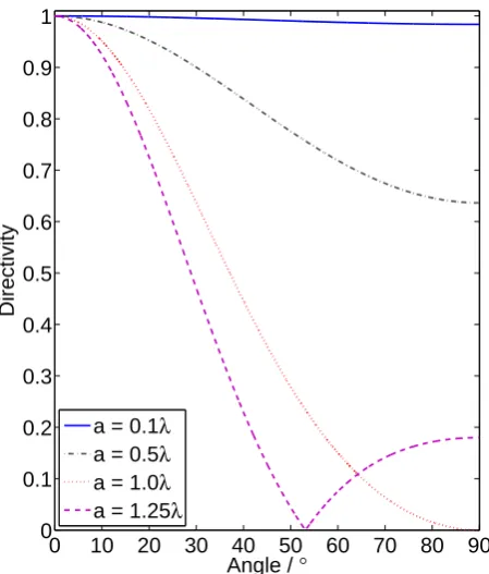
3.8 The directivity of a transducer element as the size of the element, a, is varied relative to the wavelength. . . 40

3.9 A selection of waveguide geometries which have been used to isolate piezoelectric materials from hostile environments: (a) a simple rod [1– 5], (b) a bundle of narrow rods [6, 7], (c) a threaded rod [4], (d) a hollow cylinder [8], (e) a spiralled plate [9] and (f) a thin strip [6,10,11]. 42 4.1 A schematic diagram of the displacement of the surfaces of a thin plate due to Lamb waves. The motion of the individual particles in the plate, along elliptical paths, is also shown to demonstrate the origin of these mode shapes. . . 52

(9)

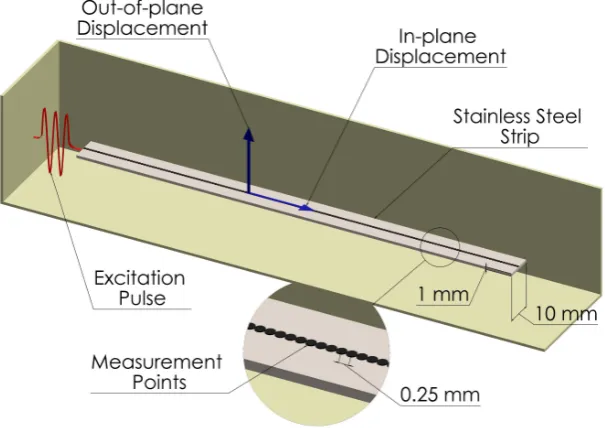
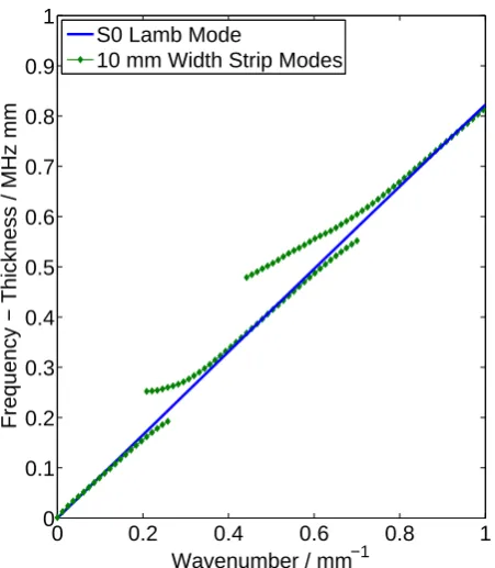
5.1 Schematic diagram of the FE model used to obtain dispersion curves. The model consisted of a single stainless steel strip driven with a nar-rowband excitation. The in-plane displacement was then measured at a series of points, 0.25 mm apart, along the centre of the strip. . . 62 5.2 The simulated dispersion curves for a stainless steel strip waveguide

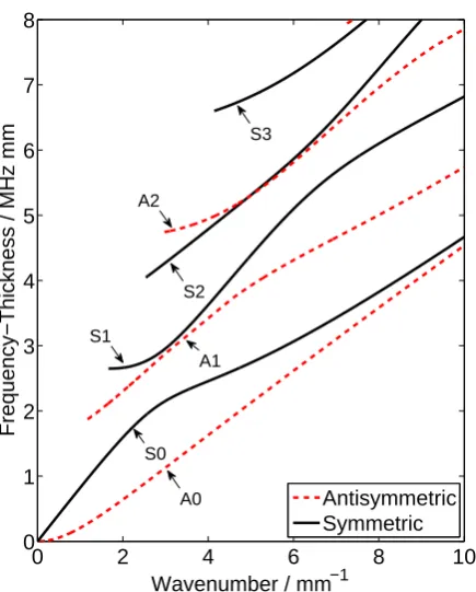
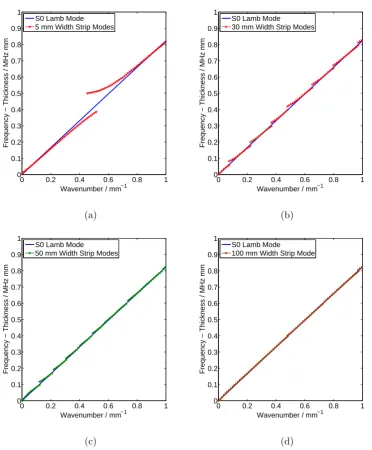
with a rectangular cross-section (1 mm x 10 mm). Also shown is the S0 Lamb mode for a 1 mm thick stainless steel plate for comparison. 63 5.3 The simulated dispersion curves for 1 mm thick stainless steel strips

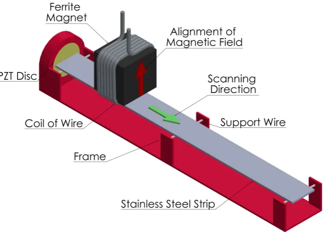
with of widths: (a) 5 mm, (b) 30 mm, (c) 50 mm and (d) 100 mm. The S0 Lamb mode for a 1 mm thick stainless steel plate is also shown for reference. . . 64 5.4 A schematic diagram of the experimental configuration used to

mea-sure the dispersion curves of a waveguide strip using an EMAT, con-sisting of a coil of wire and a magnet. . . 66 5.5 Experimentally measured dispersion curves for a 10 mm width, 1 mm

thick, 300 mm long stainless steel strip compared to those obtained from a FE model of a similarly dimensioned strip. Good agreement can be seen between the experimental data and the model. . . 68 5.6 A schematic of a waveguide strip with a taper along the length. The

front face of the waveguide where it contacts the fluid has a fixed width of 10 mm and the strip width is allowed to vary along the remaining length. . . 69 5.7 The simulated dispersion curves obtained from FE modelling of a

(10)

5.8 Front face displacement measured with a laser vibrometer for a 10 mm straight strip (top), a strip with a 0.2° taper along the length (mid-dle), and a strip with a 0.5° taper (bottom). . . 71 5.9 The frequency content of the front face displacement measured with

a laser vibrometer for a 10 mm straight strip, solid line, and a strip with a 0.5° taper along the length, dashed. . . 73

6.1 Lamb wave dispersion curves for a 316 stainless steel plate at a range of temperatures. . . 77 6.2 Schematic diagram of the experimental set-up used to investigate

the effect of the thermal gradient on wave propagation within the waveguide strips. . . 79 6.3 An example of an image of the strip taken with IR camera showing

the thermal gradient along the strip. . . 80 6.4 An example of the displacement measured at the front face of the

waveguide strip using the laser vibrometer. At the top the initial wave packet has been isolated, below a longer trace is shown which includes the series of internal reflections. . . 81 6.5 The resulting frequency spectra from applying an FFT to both the

initial wave packet, shown with a dashed line, and the whole wave train including the reverberations, shown with a solid line . . . 82 6.6 The change in average speed with increasing temperature calculated

(11)

6.7 The experimentally measured temperature profile along the length of a 1 mm x 10 mm x 300 mm strip, solid line, and the temperature pro-file from a computational fluid dynamic model of a similarly heated strip, the dashed line. . . 85 6.8 Shown here is the variation in the temperature with length between

the strip in the centre of the bundle and a strip at the edge of the bundle, inside a sealed housing. It can be seen that as the spacing between the strips is increased the variation increases. However a spacing greater than 0.8 mm causes a reduction in temperature vari-ation. . . 86

7.1 The acoustic impedance, density and velocity for stycast loaded with tungsten at a range of mass ratios. . . 96 7.2 The acoustic impedance, density and velocity for bakelite loaded with

tungsten at a range of mass ratios. . . 97 7.3 A schematic diagram of the FE model used to study the effect of

the matching layer thickness on the emitted pressure from a stainless steel waveguide. . . 99 7.4 The effect of matching layer thickness on the emitted amplitude for

stycast, bakelite and their loaded counterparts from FE modelling. 100 7.5 The affect of the waveguide length on the optimum matching layer

thickness. . . 102 7.6 A schematic diagram of the experimental set up used to measure the

emitted pressure from the waveguide assembly. . . 103

(12)

8.2 The directivity profile from 2D FE model of the five element strip waveguide array transducer with a pitch of 1.25 mm, steered to (a) 0°, (b) 10°, (c) 20° and (d) 30°. . . 111 8.3 A schematic diagram of the individual elements in the strip array,

consisting of a stainless steel waveguide strip and a cylindrical piezo-electric element. . . 114 8.4 The displacement of the front face of the waveguide strip, driven

with a thickness mode of a piezoelectric element, top, and the radial displacement of a cylindrical piezoelectric element, bottom. . . 115 8.5 The frequency content of the displacement signals when the strip

waveguide is driven with a thickness mode piezoelectric element, top, and when driven with the radial motion of a cylindrical piezoelectric element, bottom. . . 116 8.6 A simplified block diagram showing the operation of the LF-PAC. A

PC is used to program the waveform generated by the FPGA on the TxGEN board. The FPGA has 16 channels of output. Each of these channels includes a pair of differential signals and a separate analogue voltage signal. . . 117 8.7 Digital differential signalling and transformer secondary output voltage.118 8.8 Transducer voltage generation circuit. The output pulse amplitude

(13)

8.9 A schematic diagram showing the geometry of the array with the waveguide strips positioned at an angle to one another to allow for the diameter of the cylindrical piezoelectric elements. . . 120 8.10 A schematic diagram of the experimental set up used to measure the

directivity of the strip waveguide array transducer. The five strip array was fixed whilst a wideband microphone rotated about the ra-diating face of the strip waveguide array at a distance of 200 mm. . 121 8.11 The experimentally measured directivity profile of the strip waveguide

array transducer electronically steered to (a) 0°, (b) 10°, (c) 20° and (d) 30° respectively. . . 123 8.12 The directivity profile for the five element strip waveguide array

trans-ducer electronically steered to 45°. . . 124 8.13 The displacement measured at the front face of the driven strip is

shown in the upper graph, whilst the lower graph is the measured displacement from the adjacent element in the strip waveguide array transducer. . . 126 8.14 The frequency content of the displacement measurements from a

(14)

Acknowledgments

First of all I would like to thank Dr Nishal Ramadas and Professor Steve Dixon for all of the help and support they have given me during my PhD and the many amazing opportunities they have provided me with. I would also like to thank Larry Lynnworth for his advice and input as well as Elster Instromet for the support they have provided for my project.

A big thank you goes out to everyone else, both within the Warwick Ultra-sound Group and that I have had the pleasure of sharing an office with. Special mentions go to: Sam Hill, for both his constant EMAT advice and constant enter-tainment in the office; Kevin McAughey, for all the help both with MATLAB and finding a never ending supply of funny videos and of course to Tobias Eriksson, for both our many collaborations and our many “romantic holidays”.

(15)

Declarations

(16)

Abstract

A low frequency, waveguide array transducer, for operation in hostile envi-ronments, is studied and optimised for operation in fluids. The design consists of multiple stainless steel, rectangular cross-section strips which are used to support Lamb-like guided waves, which with appropriate delays allows the steering of the emitted beam.

Wave propagation within the waveguide strips is discussed and the effect of the strip geometry on the supported wave modes is studied using comprehensive finite element modelling that is validated experimentally. Deviations from Lamb wave behaviour is observed due to coupling that occurs across the finite width of the strip, leading to dispersive behaviour that is slightly different to that of Lamb waves in a plate of the same thickness. As a result of this study, suggestions are made for modifications to the waveguide geometry that may favourably change this dispersive behaviour, over a desired frequency range.

The effect of thermal gradients on the propagation of ultrasonic waves within the waveguide strips is also studied. Using Lamb waves as a basis for the analysis, general trends in the wave behaviour were identified before a series of experiments were conducted to demonstrate similar effects in the waveguide strips. Computa-tional fluid dynamics models were also used to study the heat distribution within the waveguide strips of the transducer to allow the influence of these effects in a practical application to be assessed.

(17)

Abbreviations

2D-FFT Two-Dimensional Fast Fourier Transform CFD Computational Fluid Dynamics

CMUT Capacitive Micromachined Ultrasonic Transducer EMAT Electromagnetic Acoustic Transducer

FE Finite Element

FPGA Field Programmable Gate Array FWHM Full Width at Half Maximum IR Infra-Red

ITMF In-Line Thermal Mass Flow

LF-PAC Low Frequency Phased Array Controller MEMS Microelectromechanical System

NDT Nondestructive Testing PZT Lead Zirconate Titanate

(18)

Chapter 1

Introduction

1.1 Motivation

(19)

may eventually lead to the PZT becoming depoled, and ceasing to function entirely. The a common approach to solving this issue involves placing a buffer be-tween the sensitive piezoelectric element and the hostile environment to thermally isolate the PZT. Several constraints are immediately placed on the design of such a buffer from conception. Firstly, the target environment; the buffer material must be robust enough to survive in the extreme temperatures, high pressures and poten-tially corrosive conditions of the test fluid. Secondly, the buffer must suitably isolate the sensitive piezoelectric element from the target environment, while retaining a reasonable size (say below 500 mm length) which constrains the material selection based on its thermal conductivity. These criteria usually limit the possible mate-rial selections to either a metal or a high temperature ceramic, with titanium and stainless steel being commonly chosen [12]. Additionally, for many applications it is desirable that the addition of the thermal buffer has a minimal impact on the transmitted ultrasonic waves, both in terms of pulse shape and amplitude. This limits the modifications that would be required to the standard data processing techniques that are used to obtain the flow information from the measurements. It is therefore common to design the buffer in such a way that it can support guided waves, with minimal dispersion. This is usually achieved using designs based on two geometries: either thin rods or thin plates [1–7]. These constraints will for the basis of the transducer design discussed in this thesis.

1.2 Aims and Contributions to the Field of Ultrasonics

(20)

has been studied together with the influence of the waveguide geometry on the prop-agation of ultrasound. This will assist in the design of such waveguides, allowing optimisation of the waveguide to suit ultrasonic waves of a particular frequency, for each specific application.

In addition to the protection provided by the thermal buffer, the multiple waveguide strip design can facilitate the operation of the transducer as a phased array. Ultrasonic waves may be generated in each of the strips individually with arbitrary delays. This provides the possibility of steering the emitted wave front, allowing both electronic correction of the beam path in high flow conditions and the ability to interrogate multiple paths through the test fluid using only a single pair of transducers. Due to the low wave velocities and frequencies often associated with operating in fluids, such as air, constructing a phased array transducer which satisfies the traditional array design rules is difficult; large piezoelectric elements are often required with a small array pitch. The use of waveguides in the transducer presented in this thesis allows the array to approximately satisfy these constraints, at frequencies as low as 150 kHz operating in air. The geometry at the radiating face may be different from the geometry at the other end of the waveguides where the piezoelectric material is mounted. This allows for both a simpler construction and improvements to the beam profile from the array.

1.3 Outline of Thesis

(21)

final conclusions.

In Chapter 2, a general introduction to industrial flow measurement will be given. In this chapter a range of current flow measurement techniques will be discussed, including mechanical, electromagnetic, thermal and ultrasonic methods. From this, the benefits offered by the use of ultrasonic methods will be demonstrated, as well as highlighting the issues with current methods, many of which may be dealt with using the transducer that will be described in this work.

Chapter 3 introduces several of the most common methods of generating and detecting ultrasonic waves. The primary focus of the chapter will be on the use of piezoelectric materials as this is the most common method used in the work. How-ever, other techniques which rely on electromagnetic effects and lasers will also be discussed. This chapter aims to give an introduction to both the operating principles of each of these methods as well as the strengths of each method, factors which were considered when determining which techniques to use in each experimental section of this thesis. Ultrasonic arrays will also be introduced in this chapter detailing the theory of generation using an array transducer and the design constraints which will be used later in Chapter 8.

Analytical models of the propagation of ultrasonic waves will be discussed in Chapter 4. This will begin with the general case of propagation of waves in bulk solids and fluids. This will then be developed into a description of Lamb waves. This model will be used as a simplified version of the waveguide strips used in the array transducer, allowing the general trends in wave propagation for the more complex strip waveguides to be identified. This chapter will also introduce dispersion curves, a clear understanding of which will be essential for the following chapters.

(22)

influence of the strip geometry on propagation within the waveguides was studied. Additionally, experimental validation of these finite element models is also presented. Thermal effects on the propagation of guided waves will be discussed in Chapter 6. The thermal gradient that would be produced along the length of the waveguide strip will cause variations in wave speed. To begin, an analytical model of a heated plate was used to identify the general trends expected in the behaviour of the guided waves, followed by an experimental study of with a single strip with a range of thermal gradients along the length. In addition to this, a computational fluid dynamics model will be discussed, which was used to identify any variation between the individual strips in the array when heated, as this could interfere with the phased array operation of the array.

In Chapter 7 the design of a matching layer for this transducer is discussed. The use of a stainless steel waveguide allows the isolation of the piezoelectric el-ements from the test fluid. However, it also causes a large mismatch in acoustic impedance, between the waveguide material and the target fluid. Several materials are suggested as potential matching layers, with both a suitable acoustic impedance and thermal resistance. These materials were then characterised and their proper-ties tailored, forming a composite material by loading them with other materials in order to optimise transmission into water, which was selected as a test fluid. Each of the materials was then evaluated in terms of their effectiveness as a matching layer, using both finite element modelling and experimental measurements.

(23)

transducer described in this work operates. These electronics were combined with a prototype strip waveguide array transducer to demonstrate the beam steering capabilities of the array experimentally.

Finally, in Chapter 9 some overall conclusions will be drawn, along with sug-gestions of potential developments which could be made based on the work presented in this thesis.

1.4 Publications Arising from the Thesis

1. M. Laws, S. N. Ramadas, S. Dixon, and L. C. Lynnworth, A Strip Waveg-uide Array Transducer for Fluid Coupled Applications,IEEE Transactions on Ultrasonics, Ferroelectrics, and Frequency Control, (Submitted March 2015) 2. M. Laws, S. N. Ramadas, S. Dixon, and L. C. Lynnworth,Parallel strip

waveg-uide for ultrasonic flow measurement in harsh environments, IEEE Transac-tions on Ultrasonics, Ferroelectrics, and Frequency Control, vol. 62, no. 4, p. 697 - 708, 2015.

3. M. Laws, S. Ramadas, and S. Dixon,Matching layers design for a plate waveg-uide ultrasonic transducer for flow measurement in hostile environments, in Proceedings of 2014 IEEE International Ultrasonics Symposium, pp. 2498 -2501, 2014.

4. M. Laws, S. Ramadas, and S. Dixon,High temperature studies of a rectangu-lar cross-section waveguide for flow measurement applications, in 14th Asia Pacific Conference on Non-Destructive Testing Proceedings, 2013.

(24)

6. M. Laws, S. Ramadas, and S. Dixon,A plate waveguide design for ultrasonic flow measurements in hostile environments, in Proceedings of 2012 IEEE In-ternational Ultrasonics Symposium, pp. 1718 - 1721, 2012.

(25)

Chapter 2

Flow Measurement Techniques

2.1 Overview of Flow Measurement Techniques

We shall begin here with a brief description of several of the most common types of non-ultrasonic flow meters used in industrial settings. A brief introduction to the operating principle of each type will be given, along with the types of applications where such a meter may be used. Additionally the advantages and disadvantages of each type of meter will also be discussed.

2.1.1 Orifice Plates and Venturi Meters

(26)

Figure 2.1: A schematic diagram of a classical orifice meter.

recovers further downstream; however there is usually a substantial pressure loss. The mass flow rate can then be obtained by taking two pressure measurement. The first measurement is taken one pipe diameter before the plate, as the plate should have a minimal effect on the flow at this distance. The second pressure measurement is usually taken at a distance of half a pipe diameter after the plate, which would be inside the recirculation zone. The mass flow rate can then be calculated from the pressure drop between these two measurements [13].

(27)

Figure 2.2: A schematic diagram of a classical Venturi meter.

(28)

Figure 2.3: A schematic diagram of a classical turbine meter.

are measured to allow the calculation of the mass flow rate. As before, the first measurement is taken in a region before the meter, however the second pressure measurement is taken in the throat region, where the velocity is highest and the pressure variation is greatest.

Like an orifice plate, venturi flow meters may be used with a wide range of fluids, including many multi-phase fluids [16, 17]. The main advantage of this type of flow meter rather than a simple orifice plate is the conservation of energy across the meter, which can be beneficial in some applications. This comes at the cost of increased complexity, affecting both the cost of manufacture and ease of installation.

2.1.2 Turbine

(29)

to mechanical wear. A range of electromagnetic methods may be used for this monitoring, including the detection of variations in a magnetic field due to the motion of the blades and optical methods where the motion of the blades physically blocks a beam of light [20,21]. Regardless of the specific technique used, the rotation of the rotor is converted into a series of electrical pulses which may then be used in the calculation of the flow velocity.

Turbine meters can be manufactured relatively cheaply and can be quite compact, when compared to other types of meters. Whilst the pressure loss across a turbine meter is less than that of an orifice plate it can still be significant [13]. The design of such a meter is also quite complex as the drag from the blades and the central hub of the rotor as well as the bearing must be accounted for in order to allow calculation of the flow [22–24]. Ultimately, the disadvantage of this type of flow meter is the susceptibility of the components to mechanical wear, leading to degradation in accuracy and eventual failure of the meter. This can be a particular issue when the fluid is of a non lubricating nature, which may lead to the need for regular maintenance.

2.1.3 Coriolis

(30)

[image:30.595.162.482.147.353.2]

Figure 2.4: A schematic diagram of a U-shaped coriolis meter.

the fluid combined with this vibrational motion gives rise to a coriolis force, which acts in opposite directions on the two sides of the U-shaped pipe, with the first half forced down and the second half forced up, causing the pipe to twist. Of course, during the second half of the vibrational cycle both the direction of the vibrational motion and the forces will be the opposite of those shown in figure 2.4. The de-flection caused by this twisting motion can be measured, often with some type of magnetic position sensor, allowing the flow rate to be measured.

(31)

[image:31.595.203.402.134.303.2]

Figure 2.5: A schematic diagram of a vortex-shedding meter.

discussed meters, coriolis techniques can suffer from large pressure drops, depen-dent on the application [26]. Maintenance can also be an issue with some of the more complex geometries, as removing blockages in the pipes can become problem-atic. Large thermal variations can also change the material properties of the meter, changing the distortions, which can add uncertainty to the measured velocity, if not also accounted for.

2.1.4 Vortex-Shedding

(32)

Figure 2.6: A schematic diagram of a electromagnetic meter.

velocity. A wide range of designs have been used for the bluff body, from simple cylinders to T-shapes and even more complex designs with multiple bodies [29, 30]. Low flow velocity limits the use of this type of meter, as at these velocities too few measurable vortices will be generated and the accuracy of the measurements would come into question. Vortex-shedding meters are also susceptible to errors from vibration of the pipes and pulsation of the fluid, both of which can interfere with the accurate measurement of the vortex-shedding frequency. However, if these problems can be avoided, such a meter can be a robust option for a wide range of fluids and, depending on the type of sensor used, temperatures.

2.1.5 Electromagnetic

(33)

on Faraday’s law of induction to allow the measurement of the flow of a conducting fluid, with the benefit of having no moving parts and a minimal impact on the flow. Such a flow meter has two main components, a pair of field coils which generate an, ideally uniform, magnetic field through the pipe, and a pair of electrodes aligned perpendicularly to the magnetic field, as shown in figure 2.6. As the conducting fluid flows through the field a voltage is generated across the pipe between the two electrodes. The magnitude of this voltage has been shown to be linearly proportional to the mean velocity of the fluid, allowing the velocity to be easily measured by monitoring the voltage between the pair of electrodes.

For the flow meter to function correctly the pipe material must be non-magnetic (for example some type of austenitic steel) to allow the field to penetrate the pipe wall. Additionally the interior of the meter must be lined with an electrically insulating material to prevent the generated voltages from shorting. Commonly used liner materials include rubber, neoprene, PTFE and a range of other polymers and ceramics [13]. These liner materials are susceptible to wear over time, which would damage the meter, so selection of the correct liner material for the fluid is essential, though additional techniques have been developed to enhance the longevity of the liner material [35]. Another limit on the potential applications often imposed by the liner material is the operating temperature, as the most commonly used materials are only suitable up to around 200°C [14, 36].

2.1.6 Thermal

(34)

Figure 2.7: A schematic diagram of a ITMF meter.

containing only a temperature sensor, is positioned a small distance away, but often in the same pipe cross-section. The temperature difference between the two probes is measured and electronically fixed. As the fluid flow is increased a greater amount of heat is absorbed by the passing fluid, to retain the fixed temperature difference the more power must be supplied to the heater. By monitoring the power supply to the heater it is possible to calculate the mass flow rate.

(35)

[image:35.595.170.453.146.355.2]

Figure 2.8: A schematic diagram of an ultrasonic Doppler meter.

2.2 Ultrasonic Flow Measurement Techniques

As the focus of this work is designing a transducer for ultrasonic flow measure-ment, the discussion of these techniques will be in greater depth than the previously mentioned techniques, with particular focus on the time transit technique.

2.2.1 Doppler

(36)

outside of a pipe, shown in figure 2.8. The transmitting element generates ultrasonic waves which pass through the pipe wall and in to the fluid. For a Doppler meter to function there must be some type of reflectors in the fluid, such as gas bubbles or suspended particles, which can reflect the incident ultrasonic waves back towards the sensor. The reflected ultrasonic waves are then detected by the second transducer and the frequency shift can then be used to determine the velocity of the scatterers. In application it is rarely this straight forward, as the reflecting particles would have a distribution of velocities, there is a range of angles at which the transmitted ultrasonic wave will interact with the particles in the fluid and additional effects due to the surrounding pipe geometry which results in a broadening of the frequency spectrum of the signal [37]. As such, the mean velocity of the fluid must be calculated form an estimation of the mean shift, accounting for these factors, which can lead to large uncertainties in the measurements. Additionally, with Doppler flow meters it can be difficult to know which region of the flow is being probed, as this is dependent on both the distribution of the reflectors and the attenuation of the ultrasonic signal. Thus, relating the velocity measured using this technique to the mean velocity of the fluid in the pipe a non-trivial issue. Another problem that may occur is that the reflecting particles may be propagating at a different velocity to the surrounding fluid.

2.2.2 Transit Time

(37)

Figure 2.9: A schematic diagram of an ultrasonic transit time meter.

discussing the wetted type, but many of the details being discussed are applicable for both types.

In order to obtain a flow measurement, an ultrasonic pulse is first transmitted from one of the transducers along the path, L shown in figure 2.9, and is received on the opposite transducer, and the transit time is recorded. A second pulse is then transmitted with the roles of the two transducers reversed and a second transit time obtained. With no flow, these transit time measurements should be identical, t=L/c, wherecis the sound speed in the fluid. However, when the fluid is in motion with a velocity vf it can be resolved such that it has a component along path L,

effectively modifying the sound velocity depending on if the ultrasonic waves are travelling upstream or downstream giving the following:

tup=

L

c−vfcosθ

(2.1)

tdown=

L

c+vfcosθ

(38)

These equations may then be combined to obtain an expression for the flow velocity:

vf =

L 2 cosθ

1 tdown − 1 tup . (2.3)

By eliminating the sound speed,c, from these equations the measurement becomes independent of pressure, temperature and the composition of the fluid and purely dependent on the geometry of the meter and the accuracy of the time measurements. In addition to calculating the flow velocity the two time measurements can also be used to calculate the sound speed in the fluid:

c= L

2 1 tdown + 1 tup . (2.4)

This additional information can be used to assist in the calibration of the meter [38]. In many applications, such as the petrochemical industry, it is usually desired that the mass flow rate is obtained, rather than the flow velocity. It may seem that this may be obtained my multiplying the flow rate calculated using equation 2.3 by the cross-sectional area of the pipe, and the density of the fluid, however this would only yield an accurate value if the flow profile was uniform. In most real applications this is not the case, and as such, the velocity calculated using equation 2.3 is in fact the mean velocity of the fluid along the path L. Assuming this path crosses the centre of the pipe this can cause the mass flow rate to be over estimated by as much as 33 % [39, 40]. To obtain an accurate value for the mass flow rate an additional correction factorK must be included which compensates for the profile of the flow along the particular path. This leads to the following expression:

Qm =

L 2 cosθ

1 tdown − 1 tup

AKρ(P, T), (2.5)

whereQm is the mass flow rate,Ais the cross-sectional area of the pipe andρ(P, T)

(39)

ThoughK can be used to correct for this variation, there is still an inherent uncertainty associated with the value, due to assumptions made about the profile of the flow in the pipe. One way in which this uncertainty may be further reduced is to use transit paths offset from the centre of the pipe, which has been shown to give more accurate measurements for a range of flow profiles [41].

An additional way that the uncertainty of the measurement may be reduced is by the use of multiple pairs of transducers to take measurements along several different paths. Each of the paths will give a different velocity value. The informa-tion from these paths may then be used to obtain a more accurate representainforma-tion of the flow profile, allowing more precise correction factorK to be obtained. Multiple path flow meters also allow other details about the flow to be obtained. There is no limitation to direct paths, many multiple path meters include paths with one or more reflection off the pipe wall, which allow addition features of the flow, such as swirl and asymmetry to be investigated.

(40)

2.3 Issues with Current Ultrasonic Methods and

Opportunities

Transit time ultrasonic meters are not without issue though, bubbles and particulate matter in the fluid can attenuate the ultrasonic waves, preventing the signal from being detectable at the other end of the path and making a measurement impossible, which limits the application. High flow rates can also pose an issue for transit time meters, as this can cause beam drift, where ultrasonic waves are carried in the direction of flow [42–45]. This is a particular issue in large diameter pipes and gas applications, where the sound speeds are lower and the transit times are larger, allowing the fluid velocity to have a greater effect. In many cases this beam drift will result in reduction in the amplitude detected, as only the edge of the beam will reach the detector. In more extreme cases the transmitted beam can entirely miss the transmitter. This is particularly common when there are multiple reflections in the path between the transmitter and receiver, as even a small shift in the incident angle on the pipe wall can significantly alter the beam path.

The transducer design discussed in this thesis uses an array of waveguides, allowing electronic steering of the transmitted beam. This could be used for multiple applications. Firstly, the steering could be used to correct for beam drift. This would allow the operation of the flow meter at higher flow rates, even in large pipes with low sound speed gases. Additionally, as the steering angle could be varied rapidly using a purely electronics based system, it would be possible for the flow meter to find the optimum transmission angle, automatically correcting itself when the beam begins to drift.

(41)

(42)

Chapter 3

Ultrasonic Transduction

Techniques

There are a wide range of techniques available for generating and detecting ultra-sound. When operating in a fluid however the options become much more limited. All current industrial ultrasonic flow meters rely on transducers based upon piezo-electric materials, though work is currently being conducted to investigate other possible, non piezoelectric based, transducers for ultrasonic flow metering.

(43)

Figure 3.1: The perovskite structure of PZT. On the left, the symmetric structure of the PZT when the material is above the Curie temperature is shown. On the right the polarised PZT structure is shown. The central atom is shifted from the geometric centre of the unit cell, creating a net polarisation.

3.1 Piezoelectric Transduction

(44)

structure is symmetric with no dipole moment. At lower temperatures, the structure of the unit cell changes, causing the central atom to be shifted away from the centre of the structure, imparting a dipole moment on the unit. When large piezoceramics are manufactured it normally contains some form of grain structure [54], consisting of small regions polarised in the same direction, but randomly oriented relative to the surrounding grains, resulting in no net polarisation. To make a functional device these domains must first be aligned. This is achieved by applying a large DC voltage across the ceramic in the desired poling direction, often at an elevated temperature to allow easier alignment of the individual domains [55]. The temperature of the ceramic can then be reduced while the voltage is kept fixed, leaving a polarised ce-ramic. Due to the initially random orientation of the grains, a perfect alignment of the individual dipoles cannot be achieved. However a good enough alignment can be achieved to give the ceramic a net polarisation. As a result, piezoceramic materials are sensitive to elevated temperatures. As the temperature is increased, individual grains can lose alignment, causing a reduction in the effectiveness of the material even belowTC, as the individual grains retain the local alignment of their

(45)

equations which relate the electrical and mechanical properties of the material [56]:

D=dT +TE, (3.1)

S =sET+dtE. (3.2)

HereD is the electric displacement,T is the elastic stress,T is the permittivity of

the piezoelectric material under a constant stress, E is the electric field, S is the elastic strain, sE is the mechanical compliance in a constant electric field and dt

is the transposed piezoelectric charge constant, the ratio of the applied mechanical stress and the generated electric polarisation.

Many models exist which relate the electrical input to the mechanical re-sponse of practical piezoelectric devices. This is often achieved by constructing an equivalent circuit, using some arrangement of resistors, capacitors and induc-tors [57–59]. One of the key points of these models is the presence of resonances at which a particular piezoelectric would most efficiently convert electrical energy to mechanical energy. The mathematical equations, and associated derivations, which describe the frequencies at which these resonances occur will be omitted here, however they may be found in many textbooks on the subject of piezoelectric ma-terials [51, 60].

(46)

Figure 3.2: The thickness resonances of a piezoelectric crystal demonstrated as a superposition of waves. The two edges of the PZT oscillate symmetrically about the centre of the element, with the yellow wave travelling to the left and the black wave travelling to the right. When the thickness of the PZT is equal to an odd multiple of half wavelengths the waves constructively interfere within the element, giving rise to an enhancement in the efficiency of the transducer.

waves from each of the surfaces will constructively interfere, leading to a resonance. As the width is further increased, the phase difference between the waves from each of the faces increases, until when the thickness of the block reachesλthe waves will destructively interfere [61,62]. The cycle of constructive and destructive interference will continue with increasing thickness, with additional higher frequency harmonics when the thickness of the block is equal to an odd multiple of half wavelengths:

fn=

(2n−1)c

L (3.3)

wheren= 1,2,3....and c is the sound speed in the piezoelectric material.

(47)

material and the target material. This mismatch is particularly large in fluid coupled applications, leading to large amounts of energy being reflected from the interface between the two materials. Liquids typically have acoustic impedances on the order of 1-2 MRayls, for example water has an acoustic impedance of 1.5 MRayls, com-pared to PZT which is typically around 35 MRayls. Effective coupling into gases is much more difficult as gases tend to have significantly lower acoustic impedances, for air 0.43 kRayls, giving a mismatch of approximately 5 orders of magnitude. Of-ten this effect is minimised by the addition of a matching layer with an intermediate impedance to the front of the piezoelectric material, this will discussed in more de-tail in Chapter 7. In applications where the piezoelectric material is radiating into a solid, there is an added issue of coupling. In almost all such applications some type of couplant material, usually a liquid or gel, is required to allow the ultra-sound to be transmitted effectively into the test medium, as even a thin layer of air can significantly reduce the effectiveness of the transducer. This can also lead to inconsistencies in measurements if there is variation between the coupling of the piezoelectric element.

3.2 Electromagnetic Transduction

Electromagnetic acoustic transducers (EMATs) provide a non-contact technique for generating ultrasound in an electrically conductive solid. Though EMATs may not be ideally suited to flow applications as they are unable to generate ultrasound in a fluid directly, they have been used several times in this work to both generate and detect ultrasonic waves in the metallic waveguide strips, in Chapters 5 and 7. As such it is beneficial to explain the principles of EMAT operation here.

(48)

Figure 3.3: A schematic diagram of the structure of a EMAT.

(49)

Detection of ultrasonic waves using EMATs also occurs via the Lorentz force mechanism. The incident wave causes the material in the sample to oscillate, both the nuclei and electrons. The presence of the large static magnetic field causes the motion of these particles to generate a Lorentz force which acts upon them, causing them to accelerate. This acceleration gives rise to an electric field, which in turn induces a current in the coil of an EMAT placed close to the surface. As the electrons have a much smaller mass than the nuclei the Lorentz force will cause them to experience a much greater acceleration, making the electrons primarily responsible for EMAT detection of ultrasonic waves. Much like when generating ultrasonic waves with an EMAT, the alignment of the coil relative to the magnetic field changes the direction in which the EMAT is sensitive to the motion of the electrons, allowing both the in-plane and out-of-plane velocities of the electrons to be probed separately. EMAT detection of ultrasonic waves is often more efficient than generation, as both the electrons and nuclei are set in motion by the incident wave, removing the need for momentum transfer between the two by way of collisions.

As EMATs use electromagnetic waves to transmit and detect ultrasound there is no need for any additional couplant material and EMATs can even func-tion effectively with a small lift-off between the transducer coil and the sample surface [64–66]. However, EMATs are much less efficient than piezoelectric based transducers, requiring large currents to generate ultrasonic waves, which can prevent the use of EMATs in some applications, both due to the high power requirements and the potential dangers related to high currents.

3.3 Electrostatic Transducers

(50)

mem-Figure 3.4: A schematic diagram of the structure of a CMUT.

brane with a thin electrode suspended over a doped silicon substrate, which acts as the second electrode, with a small vacuum filled cavity between the two. A cross-section of a CMUT cell is given in figure 3.4, along with some dimensions intended to give an indication of the sizes involved in CMUT devices [68]. To generate ultrasonic waves a DC bias is applied to the electrodes, causing the membrane to be attracted towards the substrate which is resisted by stresses in the membrane. An additional AC voltage is then applied which causes the membrane to oscillate. Detection with a CMUT also requires a DC bias voltage. An incident ultrasonic wave causes the membrane to oscillate, which produces a current as the capacitance of the CMUT varies while subjected to a fixed DC voltage across the electrodes.

(51)

simple to consistently produce in large quantities as they use the same fabrication techniques used in standard integrated circuitry [68].

3.4 Laser Generation

Pulsed lasers can provide a non-contact method for producing ultrasonic waves, generally used in solid materials, though some work has been conducted with flu-ids [72, 73]. Again, though this technique is not ideal for directly generating in a fluid; it could potentially be used in conjunction with some type of waveguide, as such it is mentioned briefly here.

Generation of ultrasound using lasers may occur as a result of two effects; thermal expansion or ablation. In both cases a high power laser beam pulse is directed at the surface of a sample. Some of the incident laser energy is absorbed by the surface of the material, with the remainder either lost via reflections or scattering. For lower laser beam energy densities, the incident laser light absorbed by the surface will cause localised heating, this will cause a rapid thermal expansion. This will create thermoelastic stresses. These stresses will lead to the generation of elastic waves in the bulk of the material, with the frequency content dependent on the duration of the laser pulse and the properties of both the target material and the laser.

Ablative laser generation functions in a similar manner, using a pulsed laser beam, however in this case the power of the laser is generally higher. This higher power laser causes the area struck by the laser beam to ablate, causing surface damage to the target material typically extending to a depth of several microns. The resulting stresses then lead to the generation of ultrasonic waves [73].

(52)

Figure 3.5: A schematic diagram of a simple laser vibrometer.

in very precise locations and on a range of surface geometries. However, the power requirements for such laser systems are high, as is the cost of the laser equipment required to generate the ultrasound. Additionally, lasers bring with them a large number of safety concerns, which can render these techniques difficult to use in an industrial setting.

3.5 Laser Detection

Though laser generation is not used in this work, laser detection of ultrasound is used throughout, in the from of laser vibrometry. Laser vibrometry has many advantages, including non-contact detection, preventing any mass loading which could influence the measurement, a wide bandwidth and precise measurement locations. Also, for detection only applications, the lasers used can be of much lower power, making them smaller, cheaper and inherently safer.

(53)

measure-ments, this beam passes through a beam splitter, forming two separate coherent beams; a measurement beam and a reference beam. The measurement beam con-tinues on through a lens which focuses the beam onto the surface of the sample in which the ultrasonic waves are to be measured. The laser is then reflected by the sample surface, the motion of which causes a shift in the frequency of the laser light ∆fD, given by:

∆fD =

2v

λ, (3.4)

wherev is the velocity of the target, andλis the wavelength of the laser.

The Doppler shifted light then passes back into the vibrometer, where it is reflected towards a photodetector. Before reaching the detector the reference beam and the measurement beam are combined at a beam splitter. At the detector, either the velocity of the target material or the relative displacement may be measured.

As an ultrasonic wave passes through the point monitored by the laser vi-brometer the length of the measurement beam path varies. This variation in the path length causes a modulation in the intensity of the combined beam given by [73]:

IT =IM +IR+ 2

p

IMIRcos

2π(LM −LR)

λ

. (3.5)

Here IT is the intensity of the summed beam; IM and IR are the intensities of the

reference and measurement beams respectively; andLM and LR are the respective

path lengths for the measurement and reference beams. The velocity and displace-ment measuredisplace-ments may then be monitoring the modulation of the intensity in time.

(54)

Figure 3.6: The element layout of a one dimensional/linear array. The array consists of several individual PZT elements, of lengthL, widthaand thicknesst, separated by a kerf ofK.

direction of the vibration to be distinguished.

3.6 Ultrasonic Phased Arrays

A phased array transducer is a more advanced method of generating ultrasound, which allows a much greater control over the emitted wavefront. An array trans-ducer is made up of multiple individual transtrans-ducer elements, each of which may be fired separately. This allows variable delays to be added to the ultrasonic waves transmitted from each of the elements, allowing the possibilities of electronic steering and focusing which have facilitated a huge range of new applications of ultrasonic techniques in fields such as NDT and medical imaging [52, 74–77]. Ultrasonic arrays may have a range of designs, including one dimensional linear arrays, two dimen-sional arrays and annular arrays. Primarily one dimendimen-sional arrays will be discussed here, as this is the simplest and most common design.

(55)

dis-Figure 3.7: A schematic diagram demonstrating steering on a 1D linear array.

tributed rectangular elements, with an inter-element spacing (also known as kerf) of K, as shown in figure 3.6. The length of each individual element, L is generally much larger than the widtha, allowing the length of the elements to be considered as effectively infinite such that the emission from the array may be considered on a two dimensional plane.

To steer the output from the array, appropriate delays, or focal laws, are calculated for each of the individual elements such that the waves from each element constructively interfere along the desired steering angle or focal point. For steering to an angleθ, the delay required for each element, ∆tn, is given by [76]:

∆tn=

nd

c sinθ+t0. (3.6)

Here, n = 0,±1,±2, ..., which refers to the position of each element in the array, relative to the central element; d is the array pitch, the separation between the centres of adjacent elements;cis the sound velocity in the target medium; andt0 is

(56)

are unphysical. To focus a linear array at a specific point, the individual element delays may be calculated using [78]:

∆tn=

rn−r0

c +t0, (3.7)

where rn is the distance between the element n and the focal point and r0 is the

distance between the central element and the focal point. Though equations 3.6 and 3.7 describe the delays required for a one dimensional array, they may be modified to accommodate steering and focusing in additional dimensions, for example in the case of a two dimensional array [79].

To allow the output from the array to be steered or focused ideally, the array would be required to have an infinite number of elements, each of which acts as a point source, which is clearly is not practical. As such the finite number of elements and finite size of each of the elements will affect the field emitted by the array and limit the ability to manipulate the field through the use of delays. A more realistic model considers each element as a line source than as a point source. This causes each element to emit waves with a preferred direction, known as the directivity of the element. This is calculated by integrating the fields of a line of point sources, radiating uniformly in two dimensions [80, 81]:

D(ω, θ) = 1

a ∞ Z −∞ Rect x a

e−ikxdx

= 1 a a 2 Z −a 2

e−ikxdx

= sinc ka 2 = sinc

πasinθ

λ(ω)

.

(3.8)

(57)

0 10 20 30 40 50 60 70 80 90 0

0.1 0.2 0.3 0.4 0.5 0.6 0.7 0.8 0.9 1

Angle / °

Directivity

[image:57.595.202.427.125.389.2]

a = 0.1λ a = 0.5λ a = 1.0λ a = 1.25λ

Figure 3.8: The directivity of a transducer element as the size of the element, a, is varied relative to the wavelength.

discussed in this work. From this equation it is clear that the width of the element, a relative to the wavelength, λ, will significantly affect the directivity of the ele-ment [82]. Whenais is small relative toλthe element will radiate almost uniformly in all directions. As ais increased, the emitted energy will become focused around θ= 0, as shown in figure 3.8. Additionally, when ais larger thanλthe term inside the sinc function can take values larger than π, which causes side lobes to occur at high angles. An example of these side lobes can be seen in figure 3.8 for the case of a = 1.25λ. Such side lobes not only divert energy away from the desired direction, but can also give rise unwanted signals. As such, when designing arrays it is desirable to have elements with a width less than one wavelength to suppress these effects.

(58)

the emission from the array is the element spacing, d. Due to the periodic nature of a typical array, constructive interference may occur between the waves emitted from adjacent elements. This causes the array to behave like a diffraction grating, with grating lobes emitted at an angle ofθG [83]:

sinθG=

nλ

2d. (3.9)

From this equation it is clear that in order to suppress these grating lobes the array should be designed such that the element spacing is less than λ/2. In many

applications ultrasonic arrays are driven with short pulses, rather than continuous wave signals, which lessens the effect of grating lobes, allowing theλ/2 condition to

be relaxed [84].

3.6.1 Waveguide Buffers

Waveguides have been in use as a thermal buffers since the 1930s, to overcome the difficulties associated with using piezoelectric materials at elevated temperatures [8]. In some of the earliest applications of such waveguides metallic cylinders were used to measure the specific heat of gaseous carbon dioxide at temperatures of up to 1000°C. Since this early work, ultrasonic waveguides with a wide array of geometries have been used in a range of applications.

(59)

Figure 3.9: A selection of waveguide geometries which have been used to isolate piezoelectric materials from hostile environments: (a) a simple rod [1–5], (b) a bundle of narrow rods [6, 7], (c) a threaded rod [4], (d) a hollow cylinder [8], (e) a spiralled plate [9] and (f) a thin strip [6, 10, 11].

waveguide [4]. Though these techniques have been shown to be effective, they have the drawback of introducing additional noise into the signal. More recent techniques attempt to retain some of these benefits, while avoiding the increased noise involve the addition of a layer of cladding around the central waveguide core [86–88].

(60)

this, waveguide transducers were developed which incorporated many of these thin waveguides into a bundle [6,7]. Such a design has been shown to remain substantially dispersion free, despite the contact between the individual rods.

In comparison to rod based waveguide buffers, much less work has been con-ducted using thin plate based waveguides, due to a range of practical limitations. In a similar manner to the rod waveguides, propagation with low dispersion requires that the thickness of the waveguide plate be small, compared the wavelength of the ultrasonic waves, exciting guided Lamb waves. However, to excite these modes it is also required that the other dimensions of the plate are much larger than the wavelength, reducing any interactions with these boundaries. Designing such a waveguide is feasible for high frequency applications, >2 MHz, where the wave-lengths are small, allowing rectangular cross-section waveguides to be used in fields such as NDT [90] with little dispersion. For lower frequency applications, such as fluid-coupled ultrasonics, where frequencies below 1 MHz are commonly used, the wavelengths are significantly larger, on the order of 10 mm for common waveguide materials. This makes designing a practical device difficult, as the width dimen-sion will generally be comparable to the wavelength, leading to some dispersive behaviour. There have been some attempts to overcome this limitation, for example by coiling the plate inside a cylindrical housing, allowing the exploitation of the plate like characteristics while allowing a large energy transfer in a small area [9]. Other plate based designs, instead utilise shear waves inside the waveguide in an effort to avoid dispersive behaviour. These designs have been shown to be usable in air coupled flow metering applications [6, 10, 11].

3.7 Conclusions

(61)

(62)

Chapter 4

Ultrasonic Wave Propagation

In the previous chapter a range of methods of generating and detecting ultrasound were introduced. This chapter will be concerned with how ultrasonic waves propa-gate once they have left the transducer and entered another material. When consid-ering propagating ultrasonic waves there are two fundamentally separate categories of waves which should be considered, bulk waves and guided waves [51, 91, 92]. The majority of this work will be concerned with guided waves, but to be able to un-derstand guided waves, it is useful to start with an introduction to the general case of bulk waves. In this chapter bulk waves in both solids and fluids will be dis-cussed, followed by an introduction to Lamb waves, a group of guided waves that can propagate in thin plates.

4.1 Ultrasonic Waves in Bulk Media

(63)

4.1.1 Bulk Waves in Elastic Solids

An ultrasonic wave propagating in a solid may be considered as a deformation resulting from the application of a force. At a particular point in time, this defor-mations may be described by the strain,, and stress,σ, tensors respectively, which in Cartesian coordinates may be written as [51]:

=      

11 12 13

21 22 23

31 32 33

      , (4.1) σ =      

σ11 σ12 σ13

σ21 σ22 σ23

σ31 σ32 σ33

      . (4.2)

The components of strain tensor, equation 4.1, correspond to an extension in the direction of the first index, per unit length in the direction denoted by the second index. For the stress tensor, the first index corresponds to direction of an applied force and the second corresponds to the direction perpendicular to plane to which the force is applied. In the elastic regime, which is considered to be the case for solids considered in this work, these two quantities are proportional, through Hooke’s Law [91].

Hooke’s law may be obtained by expanding the stress tensor as a Taylor series in terms of the strain tensor:

σij =σij(0) + ∂σij ∂kl kl=0 kl+

∂2σkl

∂ij∂mn

ij=0,mn=0

ijmn+. . . (4.3)

When evaluated at ij = 0, the first term σij(0) ≡ 0, due to the nature of elastic

(64)

equation 4.3 to be represented as:

σij =cijklkl, (4.4)

where

cijkl=

∂σij ∂kl kl=0 . (4.5)

This is often known as the stiffness tensor and is a three dimensional representation of Hooke’s law, relating stress and strain. The general form of this can be represented as:

cIJ =

               

c11 c12 c13 c14 c15 c16

c21 c22 c23 c24 c25 c26

c31 c32 c33 c34 c35 c36

c41 c42 c43 c44 c45 c46

c51 c52 c53 c54 c55 c56

c61 c62 c63 c64 c65 c66

                . (4.6)

However, (by applying the symmetry relations for and σ) cIJ for an isotropic

material may be represented as:

cIJ =

               

λ+ 2µ λ λ 0 0 0

λ λ+ 2µ λ 0 0 0

λ λ λ+ 2µ 0 0 0

0 0 0 µ 0 0

0 0 0 0 µ 0

0 0 0 0 µ

                , (4.7)

(65)

Table 4.1: The conversion between the four index notation to the reduced, two index, notation.

I, J ij, kl

1 11

2 22

3 33

4 23 = 32 5 31 = 13 6 12 = 21

a single index, simplifying the notation [51].

Hooke’s law, equation 4.4, can then be combined with Newton’s second law,

∂σij

∂xj

=ρ0

∂2ui

∂t2 , (4.8)

wherexjindicates direction,ρ0is the density anduiis an extension in theidirection,

to obtain the wave equation. For the isotropic material previously discussed, this takes the form:

ρ∂

2_u

i

∂t2 =

∂

∂xi

(c11−c44)

∂ui

∂xi

+c44

∂2ui

∂x2

j

+c44

∂ ∂xi ∂ui ∂xj . (4.9)

This equation can be separated into two parts, one which describes longitudinal waves, and a second which describes transverse waves:

∂2_u

L

∂t2 =c

2

L∇2uL, (4.10)

∂2uT

∂t2 =c

2

(66)

where the longitudinal and transverse velocities are given by:

cL=

r_c

11

ρ , (4.12)

cT =

r

c44

ρ . (4.13)

4.1.2 Bulk Waves in Fluids

When considering wave propagation in fluids, a slightly different approach to deriv-ing the wave equations is needed, as Hooke’s Laws is no longer valid. For fluids we base our approach on pressure,P, as this is a quantity which is commonly measured experimentally. It is simplest to begin by considering only a single dimension which may later be extrapolated into the full three-dimensional case. A one dimensional force, applied to a singular volume element, betweenx andx+dx, will give rise to a pressure increase in that region:

dFx=

P(x)−

P(x) + ∂P

∂xdx

A=−∂P

∂xdxA. (4.14)

Here dFx is the change in the force in the x direction and A is the cross-sectional

area of the volume element. The mass of this volume element is give by ρ0dxA,

which allows equation 4.14 to be combined with Newton’s law, to give:

∂P

∂x =−ρ0

∂2u

∂t2. (4.15)

A new term, compressibility, χ, can be defined to link the pressure change to a volume change:

χ=−1

(67)

This term can then be substituted into equation 4.15 to give an alternate form of the wave equation:

∂2u

∂t2 =V

2 0

∂2u

∂x2, (4.17)

where

V₀2 = 1

ρ0χ

= ∂P

∂ρ, (4.18)

which is the sound velocity in the fluid.

4.2 Ultrasonic Guided Waves

Unlike bulk waves, a guided wave has its energy and motion restricted by a set of boundaries. This results in the creation of an infinite number of individual propa-gation modes which may be calculated by solving the wave equation with specific sets of boundary conditions. For many applications, such as in the field of NDT, the beneficial properties of particular guided wave modes are exploited, in order to allow ultrasonic waves to travel large distances with minimal dispersion while losing minimal energy.

4.2.1 Dispersion of Guided Waves

Dispersion occurs when the velocity of an ultrasonic wave has a dependence on frequency. This is not usually an issue with bulk waves, but dispersion is common in many types of guided waves. Dispersion causes a propagating ultrasonic pulse to spread out in space and time, as the individual frequency components within the pulse propagate with slightly different velocities.

(68)

measurement, as cross-correlation is commonly used to determine transit times that are required to calculate flow rates [94]. Such distortion of the transmitted signal, introduced by dispersion in a waveguide, can increase the difficulty of obtaining an accurate measurement of a flow velocity.

Guided wave modes are not equally dispersive at all frequencies, and by selecting the correct frequency for a specific geometry it is possible to limit the dispersion of a guided wave. For many applications, thin rods and plates are often used as waveguides, as the modes in such geometries are well understood and they support modes with low dispersion regions [92].

This thesis is primarily concerned with waveguides consisting of thin metallic strips with a rectangular cross-section. It is expected that the modes supported by such strips should be similar to those in a semi-infinite thin plate. Therefore it is helpful to start by discussing guided waves in such thin plates, as they are well understood and straightforward.

4.2.2 Lamb Waves in Thin Plates

Lamb waves are a type of guided wave that can propagate in a thin plate, which are described by the Rayleigh-Lamb equations [91, 92, 95]. In order to derive these equations we must first state several assumptions about the material. Firstly, it is assumed that the material is isotropic and homogeneous. Next, the surfaces of the plate being considered should be traction free, meaning that there is no stress on these boundaries. Finally, the plate is assumed to be “semi-infinite”. In practical terms, this means that the dimensions of the plate, other than the thickness, are much larger than the particular wavelength of interest. This allows any additional boundaries to be neglected which simplifies the calculation.

(69)

Figure 4.1: A schematic diagram of the displacement of the surfaces of a thin plate due to Lamb waves. The motion of the individual particles in the plate, along elliptical paths, is also shown to demonstrate the origin of these mode shapes.

displacements about the mid plane, the A-modes, given here respectively:

tan(qa)

q +

4k2ptan(pa)

(q2₋_k2₎2 = 0, (4.19)

qtan(qa) + (q

2₋_k2₎2_tan(_pa₎

4k2_p = 0, (4.20)

where k is the wavenumber (the spatial frequency of the wave, k = 2_λπ), 2a is the thickness and the variablespand q are defined as:

p2 =

ω

cL

2

−k2, (4.21)

q2 =

ω

cT

2

−k2. (4.22)

Hereω is the angular frequency and cL and cT are the longitudinal and transverse

Low frequency strip waveguide array for flow measurement in hostile environments

University of Warwick institutional repository:

http://go.warwick.ac.uk/wrap

A Thesis Submitted for the Degree of PhD at the University of Warwick

http://go.warwick.ac.uk/wrap/77475

This thesis is made available online and is protected by original copyright.

Please scroll down to view the document itself.

Low Frequency Strip Waveguide Array for Flow

Measurement in Hostile Environments

Michael Richard Laws

Physics

Contents

List of Figures

Acknowledgments

Declarations

Abstract

Abbreviations

Chapter 1

Introduction

1.1

Motivation

1.2

Aims and Contributions to the Field of Ultrasonics

1.3

Outline of Thesis

1.4

Publications Arising from the Thesis

Chapter 2

Flow Measurement Techniques

2.1

Overview of Flow Measurement Techniques

2.2

Ultrasonic Flow Measurement Techniques

2.3

Issues with Current Ultrasonic Methods and

Opportunities

Chapter 3

Ultrasonic Transduction

Techniques

3.1

Piezoelectric Transduction

3.2

Electromagnetic Transduction

3.3

Electrostatic Transducers

3.4

Laser Generation

3.5

Laser Detection

3.6

Ultrasonic Phased Arrays

3.7

Conclusions

Chapter 4

Ultrasonic Wave Propagation

4.1

Ultrasonic Waves in Bulk Media

4.2

Ultrasonic Guided Waves