warwick.ac.uk/lib-publications
Original citation:Sanborn, Adam N. and Hills, Thomas Trenholm. (2014) The frequentist implications of optional stopping on Bayesian hypothesis tests. Psychonomic Bulletin & Review , Volume 21 (Number 2). pp. 283-300.
Permanent WRAP URL:
http://wrap.warwick.ac.uk/64309
Copyright and reuse:
The Warwick Research Archive Portal (WRAP) makes this work by researchers of the University of Warwick available open access under the following conditions. Copyright © and all moral rights to the version of the paper presented here belong to the individual author(s) and/or other copyright owners. To the extent reasonable and practicable the material made available in WRAP has been checked for eligibility before being made available.
Copies of full items can be used for personal research or study, educational, or not-for profit purposes without prior permission or charge. Provided that the authors, title and full bibliographic details are credited, a hyperlink and/or URL is given for the original metadata page and the content is not changed in any way.
Publisher’s statement:
“The final publication is available at Springer via http://dx.doi.org/10.3758/s13423-013-0518-9
A note on versions:
The version presented here may differ from the published version or, version of record, if you wish to cite this item you are advised to consult the publisher’s version. Please see the ‘permanent WRAP url’ above for details on accessing the published version and note that access may require a subscription.
Bayesian Hypothesis Tests
Adam N. Sanborn
Thomas T. Hills
Department of Psychology, University of Warwick
Abstract
Null hypothesis significance testing (NHST) is the most commonly used statistical methodology in psychology. The probability of achieving a value as extreme or more extreme than the statistic obtained from the data is evaluated, and if it is low enough then the null hypothesis is rejected. However, because common experimen-tal practice often clashes with the assumptions underlying NHST, these calculated probabilities are often incorrect. Most commonly, experimenters use tests that as-sume sample sizes are fixed in advance of data collection, but then use the data to determine when to stop; in the limit, experimenters can use data monitoring to guarantee the null hypothesis will be rejected. Bayesian hypothesis testing (BHT) provides a solution to these ills, because the stopping rule used is irrelevant to the calculation of a Bayes factor. In addition, there are strong mathematical guarantees on the frequentist properties of BHT that are comforting for researchers concerned that stopping rules could influence the Bayes factors produced. Here we show that these guaranteed bounds have limited scope and often do not apply in psycholog-ical research. Specifpsycholog-ically, we quantitatively demonstrate the impact of optional stopping on the resulting Bayes factors in two common situations: 1) when the truth is a combination of the hypotheses, such as in a heterogeneous population, and 2) when a hypothesis is composite–taking multiple parameter values–such as the alternative hypothesis in a t-test. We found that for these situations that while the Bayesian interpretation remains correct regardless of the stopping rule used, the choice of stopping rule can, in some situations, greatly increase the chance of an experimenter finding evidence in the direction they desire. We suggest ways to control these frequentist implications of stopping rules on BHT.
The standard statistical methods of psychological research, such as the ANOVA and the t-test, are examples of null hypothesis significance testing (NHST). These familiar frequentist methods compare a statistic calculated from the data, such as an F-test statistic or a t-test statistic, to a sampling distribution associated with the null hypothesis. If the probability of achieving a result
as extreme or more extreme than the one obtained is lower than a predetermined threshold–the probability of making a type I error,α–then the null hypothesis is rejected.
One of the difficulties of using NHST is that the relevant details of the experimental proce-dure, such as the reason that the experimenter stopped collecting data, are often unknown to the reader. The reported number of participants could have been collected in a variety of ways. It could be that the number of participants was fixed in advance, here called fixed stopping, or the experiment was stopped in response to the data collected, here calledoptional stopping. In the most extreme case of optional stopping, which we callpreferential stopping, researchers check the data as observations are collected and stop the experiment as soon as a significant result is acquired.
Optional stopping in these various forms is potentially quite common. In a recent survey, 58% of researchers admitted to having collected more data after looking to see whether the results were significant and 22% admitted to stopping an experiment early because they had found the result that they were looking for (John, Loewenstein, & Prelec, 2012). Participants playing the role of an experimenter have also shown high prevalence of this type of behavior (Yu, Sprenger, Thomas, & Dougherty, submitted). There are often good reasons for optional stopping. One possible reason for optional stopping is a high cost of continuing to collect more data (e.g., in fMRI experiments or medical trials), and thus early stopping following clear results can reduce the overall costs of doing research. In contrast, the data may be noisier than expected and more data may be required to observe an effect when it is present.
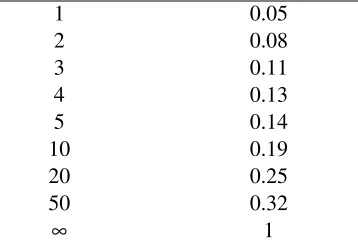
The statistical consequence of optional stopping is that, without appropriate corrections, the reported results will often be overstated. There are various NHST methods for sequential analysis of the data (e.g., Armitage, 1960; Wald, 1947), but they are rarely used. Instead, psychological researchers almost always use NHST methods that assume the sample size is fixed in advance of the experiment; this mismatch inflates the probability of erroneously obtaining a significant result when the null hypothesis is true. Table 1 (from Armitage, McPherson, and Rowe (1969) and used later in Jennison and Turnbull (1990), Pocock (1983), and Wagenmakers (2007)) gives a clear example of this inflation. Here the experimenter tests whether the mean of normally distributed data with known variance is equal to zero. The data are collected in equal-sized batches and preferential stopping is used: the test is performed after each batch is collected and if a significant result is found then the experiment is stopped. Using a test that assumes a fixed sample size, the probability of achieving a result ofp< .05 increases as a function of the number of times that the data are tested. Citing a p-value based on a fixed sample size after repeatedly checking data is a misrepresentation of the evidence and how it was acquired. Most disturbingly, the probability of a single experiment ’rejecting the null’ approaches unity with increasing numbers of tests – with NHST, experimenters who wish to reject the null hypothesis can be certain to do so if they commit themselves to collecting enough data.
Table 1: Probability of rejecting a true null hypothesis as a function of the number of tests
Number of tests Probability of rejectingH0
1 0.05
2 0.08
3 0.11
4 0.13
5 0.14
10 0.19
20 0.25
50 0.32
∞ 1
corrections are needed” (p.167).
As we review below, the Bayesian interpretation of the evidence does not depend on the stopping rule used, and thus is correct no matter the reason used to stop the experiment or whether the stopping rule is known or unknown. However, there is also the practical question of what the frequentist properties of BHT are, which govern how easy it is to produce evidence for or against a hypothesis. Indeed, some researchers have investigated the frequentist properties of the standard Bayesian hypothesis test–the Bayes factor–and found mathematical bounds on how often the Bayes factor will reach certain values. As stated by Edwards et al. (1963), ”...if you set out to collect data until your posterior probability for a hypothesis which unknown to you is true has been reduced to .01, then 99 times out of 100 you will never make it, no matter how many data you, or your children after you, may collect” (p. 239). These bounds seem to imply that BHT actually has better frequentist properties than NHST and researchers concerned about the frequency with which convincing Bayes factors could be produced can proceed without worrying about what sort of stopping rule the experimenter used. In this article, we will demonstrate that this is not always the case.
In particular, while the above quote about the bounds is correct, it applies only to very narrow situations (Mayo & Kruse, 2001; Royall, 2000, Rejoinder), situations that rarely occur in psycho-logical research. As a consequence, the above bound cannot always be used as a guide for the frequentist implications of using Bayes factors in psychological research, and it is possible that the probabilities of generating convincing Bayes factors are far higher than the quote implies. Even though Bayesian interpretations of Bayes factors do not depend on stopping rules, it may be possi-ble to use optional stopping to influence both the size and direction of the evidence produced in an experiment, which could be used by researchers, inadvertently or not, to generate results that suit their purposes. We feel it is important for researchers to understand these properties, in order to have a more complete understanding of how to best use BHT in practice.
when the true hypothesis is composite, such as the alternative hypothesis in a t-test. We investigate these cases with simulations to check how much the probabilities of generating convincing Bayes factors can be influenced by the choice of stopping rule, finding some situations in which it has a large effect and others in which the frequentist bound approximately holds. Finally, we discuss the frequentist implications of using Bayesian hypothesis tests and what techniques can be used to control the frequentist properties of these tests.
Bayesian Hypothesis Testing
BHT provides a way of evaluating two hypotheses by directly comparing how well they explain the data. To do so, a Bayes factor is computed, which gives a convenient and easily inter-pretable statistic. The Bayes factor is the likelihood ratio of two hypotheses, providing the relative probability that the data could have been produced by one hypothesis or the other. For two compet-ing hypothesesH1andH2,
BF=P(Xn|H1)
P(Xn|H2)
(1)
whereXnare the data collected overntrials. Thus, the Bayes factor tells us how much more likely it is that the data were generated by H1 than byH2. This follows from the fact that the Bayes factor is composed of a ratio of likelihood functions, which each represent conditional probability distributions associated with how likely the observed data would be given a specific hypothesis. According to thelikelihood principlethe likelihood function contains all the information relevant to inferences aboutH(Birnbaum, 1962; Hacking, 1965).
The computation of the likelihood, P(Xn|H), depends on the type of hypothesis, of which there are two types. Asimple hypothesishas no free parameters and consists of a single probability distribution defined over the possible data. For example, a coin with a fixed probability of heads (e.g., 0.55) is a simple hypothesis and one can easily compute the likelihood of any combination of heads or tails given this hypothesis. Null hypotheses can be simple hypotheses, an example of which is “the difference between two means is exactly zero1.”
The second type of hypothesis is acomposite hypothesiswith one or more free parameters, each of which can take a number of possible values. It consists of a set of probability distributions, with the values of the parameters determining which probability distribution is used. Alternative hypotheses are commonly composite hypotheses, for example, “the probability of heads does not equal one half” or “the difference between two means is not zero”. Computing the Bayes factor for a composite hypothesis makes use of a prior distribution over the free parameters. Ifθis a continuous free parameter, the priorP(θ|H1)indicates the belief in different values of the parameter before the experiment begins. Given this prior distribution, computing the likelihood is straightforward: the probability of the data given a hypothesis is essentially the average of the probabilities of the data over all values ofθ, weighted according to their prior probabilities,
P(Xn|H1) =
Z
θ
P(Xn|θ,H1)P(θ|H1)dθ. (2)
1This example is only a simple hypothesis when the variance is known. If the variance is unknown, the null hypothesis
After collecting data, the Bayes factor can be directly reported as the strength of the evi-dence in favor of one hypothesis or the other, and the Bayes factor contains all the information about the experiment needed for researchers to update their prior beliefs about the hypotheses. As we review in more detail in the Discussion, because of the likelihood principle the intentions of the experimenter or the use of certain stopping rules are irrelevant: the data are the data and the likelihoods are not subject to anything but the data (Berger & Wolpert, 1988; Good, 1982; Lind-ley, 1957). Moreover, the Bayes factor is a measure of relative evidence about two hypotheses, not an indication of how frequently a particular result would be attained given repeated experiments. The continuous nature of the evidence is perhaps confusing for researchers more familiar with the fixed p-value thresholds used in NHST. Possibly because of this, researchers have developed qual-itative labels indicating the strength of the evidence for different thresholds of Bayes factors. In what follows, we use one set of three thresholds, 3:1, 10:1, and 100:1, which have been respectively described as ’substantial,’ ’strong,’ and ’decisive’ evidence in favor of one hypothesis over another (Wetzels et al., 2011; though the somewhat arbitrary nature of label assignment has resulted in other slightly different schemes: Jeffreys, 1961; Kass & Rafferty, 1995; Royall, 1997).
Optional Stopping and the Universal Bound
A often-cited frequentist guarantee for Bayes factors is that there is a bound on how often any stopping rule, including preferential stopping, can result in evidence that supports a false hypoth-esis over the true hypothhypoth-esis (Birnbaum, 1962; Kerridge, 1963; Robbins, 1970; C. Smith, 1953). Because of its generality, this is known as theuniversal bound(Royall, 2000). Let us assume that an experimenter preferentially stops the experiment as soon as the Bayes factor reaches the value
k in support of his favored hypothesis, where k>1, or otherwise continues until he runs out of resources. If the experimenter is seeking evidence for the false hypothesis over the true hypothesis, the probability that he will be successful, no matter how long he continues, has a maximum upper limit,
p
P(Xn|F)
P(Xn|T)
>k
≤ 1
k (3)
whereFis the false hypothesis andT is the true, or data-generating, hypothesis. Thus, if an experi-menter aimed to find 10:1 evidence favoring a false hypothesis over a true hypothesis, in only 10% of all experiments could preferential stopping achieve this goal. This is certainly an advantage over NHST (see Table 1), for which the chances are 100%.
The proof of the universal bound is reproduced in the Appendix, and it holds for any stopping rule. It is the basis for the quote by Edwards et al. (1963) in the introduction, stating that no matter how long an experiment is run and no matter what stopping rule is used, there is a high probability that strong evidence for the false hypothesis can never be obtained. Even for the weakest criterion we consider, 3:1, there is only a 1/3 chance that the experimenter will ever be successful in stopping with evidence against a true hypothesis. This bound on the frequency of obtaining particular Bayes factors is a powerful tool for researchers interesting in controlling the frequentist implications of BHT.
literature (Mayo & Kruse, 2001; Royall, 2000, Rejoinder), but here we investigate the quantitative consequences of the limitations as well as go into greater depth as to where the universal bound remains a good guide. In the following two sections we explore the consequences of preferential stopping when the universal bound’s assumptions are not satisfied. In both sections, we demonstrate the violation first with a coin flipping example and then with a more practically relevant example from the psychological literature.
When the Truth is a Combination of the Hypotheses
Researchers often propose hypotheses that reflect a particular theoretical outlook. For exam-ple, researchers might believe that people are using heuristic or rational models of decision making (Gigerenzer & Todd, 1999; Lee & Cummins, 2004), or perhaps they are using an exemplar or proto-type representation to generalize their experiences (Medin & Schaffer, 1978; Nosofsky, 1986; Reed, 1972). These hypotheses are tested against one another to explain empirical data, but it is commonly understood that in describing such a complex system as the mind, no theory is ever completely true (Nester, 1996). It could well be that the population is heterogeneous, and that some hypotheses describe some individuals but not others. Indeed, it has been found that some individuals are bet-ter described by heuristics and others by more compensatory decision strategies (Lee & Cummins, 2004) and some individuals better described by a prototype model and others by an exemplar model (Bartlema, Lee, Wetzels, & Vanpaemel, submitted). Heterogeneity can occur even within an in-dividual: people can use different strategies at different times (e.g., Rieskamp & Hoffrage, 2008). Researchers often test “pure” hypotheses, while the true generating model might be a mixture of the hypotheses under consideration: for some trials or individuals one hypothesis is true and for the remaining trials or individuals the other hypothesis is true.
A related possibility is that the true generating model is actually an integrated combination of both of the hypotheses under consideration. One relevant example is human estimation of the joint probability of two independent events. The normative rule is to multiply the probabilities of the independent events together, but some researchers have instead proposed that people respond with the weighted average of the probabilities of the two independent events (Fantino, Kulik, Stolarz-Fantino, & Wright, 1997; Nilsson, Winman, Juslin, & Hansson, 2009). The normative rule and the weighted average rule are the usual hypotheses that are compared in these experiments. How-ever, other researchers have found that the best fitting model is an average of these two hypotheses (Jarvstad & Hahn, 2011; Wyer, 1976). In general, the behavior produced could well be a weighted average of the behavior predicted by each of the hypotheses, that is, the data generating hypothesis may be an integrated combination of the two hypotheses considered.
Deciding Between Two Biased Coins
Our first example will test between two specific hypotheses about the bias of a coin and investigate the frequency of achieving Bayes factor thresholds for a range of different biases that are not necessarily equal to the hypotheses that are considered. One of the hypotheses,CH, is that the coin is biased towards producing heads, withP(H|CH) =0.75. The other hypothesis,CT, is that the coin is equally biased towards producing tails, whereP(H|CT) =0.25. Given that the experimenter independently flips a coin n times, the probability of s heads for either of these coins follows a Binomial distribution,
P(s|n) =
n s
P(H)s(1−P(H))n−s. (4)
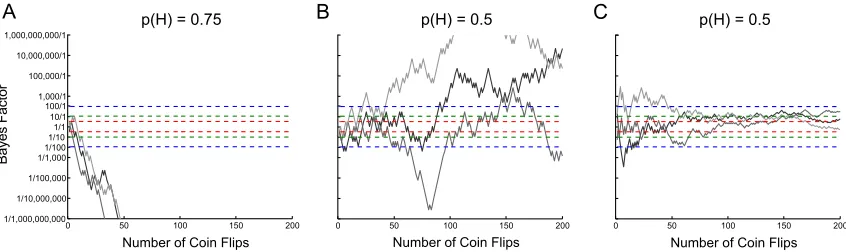
Suppose that data are generated such that each hypothesis is a combination of the hypotheses, either meaning that one of the two coins from the hypotheses is selected randomly with some proba-bility on each trial, or (equivalently as we have shown) that a single coin with a bias that lies between the two hypotheses is flipped on every trial. Letwindicate the weight for each hypothesis, with the probability of heads in the data beingP(H) =wP(H|CH) + (1−w)P(H|CT). Figure 1A shows how the Bayes factors change as the data are collected for three sample experiments, with each path showing the trial-by-trial value of the Bayes factor as the heads and tails are accumulated. These paths are shown relative to the thresholds for substantial, strong, and decisive evidence for each hypothesis. We show two cases: one for whichCHis true (P(H) =0.75) and one for whichw=0.5 (the two hypotheses are equally weighted and the coin is fair). WhenCH is true andP(H) =0.75, the assumptions of the universal bound hold. The Bayes factor for each example experiment drifts rapidly toward dominance for the true hypothesis and only 1/3 of the sample experiments exceed the 3:1 threshold for the false hypothesis. This example illustrates the principle ofconsistency: as the amount of data increases the Bayes factor converges on the correct hypothesis.
For w=0.5 and P(H) =0.5 in Figure 1B the evidence lies exactly between the two hy-potheses on average, and for these two models, neither of which generated the data (or includes a component that generated the data), the consistency principle no longer holds. Here the Bayes factors in the sample experiments do not remain close to the indifference line of 1:1, but instead swing wildly as the data accumulate: the Bayes factor for a single experiment can at times favor one hypothesis decisively and later favor the other decisively. Because neither model exactly gen-erated the data, the universal bound also no longer holds. These sample experiments illustrate the problem when truth is a combination of both hypotheses: preferential stopping would mean that the experimenter could find decisive evidence for his favored hypothesis.
0 50 100 150 200 1/1,000,000,000
1/10,000,000 1/100,000 1/1,0001/100 1/10 1/1 10/1 100/1 1,000/1 100,000/1 10,000,000/1 1,000,000,000/1
Number.of.Coin.Flips
B
ay
es
.F
ac
to
r
0 50 100 150 200
p(H).=.0.75 p(H).=.0.5
Number.of.Coin.Flips
A B
0 50 100 150 200
p(H).=.0.5
C
[image:9.612.95.518.89.215.2]Number.of.Coin.Flips
Figure 1. Changes in the Bayes factor as data are accumulated in example coin flipping experiments. In each plot, the three gray lines represent the Bayes factors in three example experiments. Values above one indicate evidence that favors the biased hypothesisCT and values below one favor the biased hypothesisCH. The dashed lines indicate standard Bayes factor thresholds for substantial (3:1 in red), strong (10:1 in green), and decisive (100:1 in blue) evidence. A) The probability of heads being generated is 0.75 (CHis true) where
P(H|CH) =0.75 andP(H|CT) =0.25. B) The probability of heads being generated is 0.5 (CH andCT are equally true). C) The probability of heads being generated is again 0.5, but two composite hypotheses that equally weightP(H) =0.5,CH0 withP(H|CH0 )∼Beta(20,1)andCT0 withP(H|CT0)∼Beta(1,20), are tested.
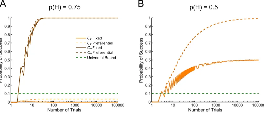
Returning to our two simple hypotheses, we investigated the probability of achieving Bayes factor thresholds systematically, by imagining two experimenters: one who prefersCH and stops the experiment if the Bayes factor favorsCHby 10:1, and the other who prefersCT and stops if the Bayes factor favorsCTby 10:1. Assume that our experimenters are willing to perform up to 100,000 coin flips, stopping the experiment as soon as the favored hypothesis reaches a Bayes factor of 10:1, but continuing otherwise. Because an experimenter can stop as soon as the threshold is reached, in many cases the experimenter will not need to collect all 100,000 trials.
Figure 2A presents the probability of success for our experimenters within 100,000 trials whenCHis true andP(H) =0.75. Here, the probability of success for the experimenter who favors the true hypothesis is near one. Alternatively, for the experimenter who favors the false hypothesis, the probability of success is quite low (<0.1). To see the advantage of preferential stopping, we compare these results to experimenters who choose the number of trials in advance of the experiment (fixed stopping rule). While preferential stopping does increase the probability of success for each of the experimenters over fixed stopping, the probability of success for the false hypothesis is far below the universal bound.
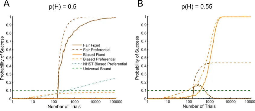
However, if each hypothesis is equally weighted, as in Figure 2B with w=0.5, the results change considerably. First, each of the experimenters who preferentially stop has a very high prob-ability of success, with either experimenter able to claim strong evidence for their preferred hypoth-esis with near certainty within 100,000 trials. Second, even using a fixed stopping rule is reasonably likely to result in evidence that strongly supports one hypothesis or the other, though the direction of the evidence is not determined in advance as it is for preferential stopping. The effect of preferential stopping can be seen as the difference between fixed and preferential stopping, which is here quite large. This is a striking departure from the case in which one of the hypotheses generated the data and the universal bound applies.
Figure 2. The probability of successfully using preferential stopping to support a hypothesis as the number of trials increases from 1 to 100,000 using a Bayes factor threshold of strong evidence (10:1). For the fixed stopping rule, the threshold is only checked at that particular trial number. For the preferential stopping rule, the probability of success is the proportion of experiments that have reached the threshold in favor of the preferred hypothesis at that particular trial or earlier. The dashed green represents the universal bound for the criterion. The jaggedness of the plots is mainly due to the discrete nature of the data, but above 100 trials not every trial is plotted, which smooths the plot. A) The probability of generating heads is 0.75 (CHis true). B) The probability of generating heads is 0.5 (CHandCT make equal contributions). The brown and orange lines lie on top of one another in this plot.
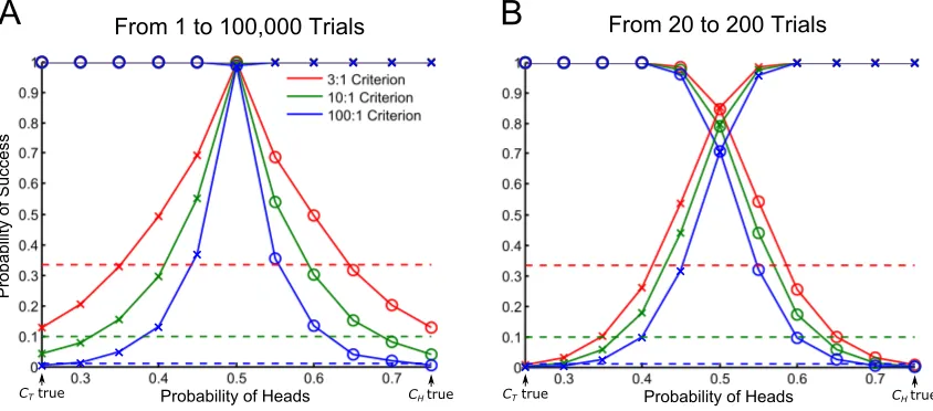
not limited to cases in which the two hypotheses are equally weighted. Figure 3A generalizes the findings of Figure 2, showing the probability of success for our two experimenters using preferential stopping, for various values ofP(H)that range betweenCH being true (P(H) =0.75) andCT being true (P(H) =0.25) and for our three threshold criteria. The universal bounds hold when one of the hypotheses is true, but the probability of generating the desired evidence rises sharply asP(H)
approaches 0.5. Critically, even when the data generating hypothesis is closer to one hypothesis, evidence that supports the other hypothesis can be generated with higher probability than one would expect if using the universal bound as a guide. For example, looking at the case ofP(H) =0.55, for which the evidence is slightly in favor ofCH, the experimenter who favors hypothesisCT will be successful more than half of the time for the strong evidence (10:1) threshold.
Figure 3. The probability of successfully using preferential stopping to find evidence forCH(x) or evidence forCT (o) given a specific true probability of heads and a specified Bayes factor threshold. The dashed lines are the universal bounds for each threshold. A) Probability of success when checking the Bayes factor after every trial from the first to 100,000th trial. B) Probability of success when checking the Bayes factor after every trial from the 20th until the 200th.
Exponential or Power Law Models of Memory Decay
The above case is artificial by design, demonstrating in a ‘toy’ environment that preferential stopping can greatly change the probability of achieving desired Bayes factors. Here we extend these findings to a problem more firmly in the domain of psychology, specifically, the mathematical description of memory. Establishing the mathematical form of forgetting (i.e., the forgetting curve) involves relating the probability of memory retention, R, to the time interval between study and test,t. The specific mathematical form of the relationship betweenRandtwas investigated more than 100 years ago by Ebbinghaus (1974), but remains an open question in memory research, with researchers comparing exponential and power law forms of memory decay (e.g., Wixted & Ebbe-sen, 1991) among other forms. Recent elegant work by Averell and Heathcote (2011) revisits this question using hierarchical Bayesian model selection to compare exponential decay and power law decay, finding evidence for power law decay. In the present analysis, we artificially place the truth somewhere between exponential and power law decay models. We have no particular reason to sus-pect that this reflects reality, but the example of forgetting functions suits our purpose by producing binary data (recalled or not recalled) and for having the tradition of testing various models against one another.
Specifically, we assume that the properties of forgetting are driven by a combination of both exponential and power-law processes. Following Averell and Heathcote (2011), we let the proba-bility of retention for exponential forgetting be
pe(t) =a+ (1−a)be−αt (5)
pp(t) =a+ (1−a)
b
(1+t)β (6)
where for both modelst is the time delay, bis the maxiumum probability of recall, and a is the minimum probability of recall.
We further assume that the observed probability of forgetting, for a given set of experiments, is a weighted function of the above two forgetting functions,
R(t) =wpe(t) + (1−w)pp(t) (7)
To simulate a typical study of this kind, we let each participant be tested for recall at five different time points (t=1,2,3,4,5). The number of items recalled at each time point was generated as the outcome of a random binomial sample with 20 possible items to recall, where the probability of recall for each item was equal toR(t), from Equation 7. We let each participant have the same underlying forgetting functions, fixing the parameters ata=0.2, b=0.8, α=.5 andβ=1. We
then simulated the outcomes of the two different experimenters as before, with one favoring the exponential hypothesis and the other favoring the power-law hypothesis. The two experimenters each collect independent data, first evaluating the Bayes factor after collecting 20 participants. From there forward, they evaluate the resulting Bayes factor after each participant until they reach the desired threshold Bayes factor, or until they have sampled 200 participants.
Figure 4 presents the probability of success for each of the experimenters, for different values ofwbetween 0 and 1. Notably, for values ofwthat are 0 or 1 and one of the hypotheses generated the data, the universal bound applies. However, for cases nearw=0.5 and neither hypothesis generated the data, in more than half of experiments preferential stopping can produce Bayes factors of up to 100:1 in support of whichever hypothesis the experimenter favors.
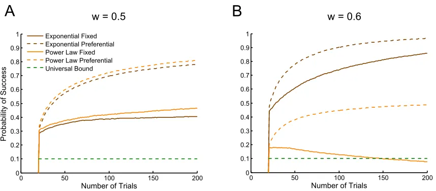
Once again, preferential stopping plays a considerable role in creating such favorable out-comes for our experimenters. As can be seen for the case ofw=0.5, presented in Figure 5A, the results for fixed stopping lie considerably above the bound, with ’strong’ evidence for each of the hypotheses more than a third of the time. However, including preferential stopping nearly doubles an experimenter’s chances of successfully finding support for their favored hypothesis. Even if the data slightly favor the exponential hypothesis (w=0.6, presented in Figure 5B), the chance of find-ing strong evidence for the power law hypothesis exceeds 10% for small numbers of trials and is greatly increased by preferential stopping.
Though the present case is still artificial in many respects (e.g., using simple hypotheses, meaning that each parameter is fixed), assuming more realistic scenarios – such as participants with different shaped forgetting functions and performing a hierarchical Bayesian analysis to account for heterogeneous behavior – does not remove the problem. Indeed, introducing free parameters (i.e., composite hypotheses) also violates the assumptions used to derive the universal bound. However, before we examine the consequences of introducing such composite hypothesis, we first briefly discuss the bounds on generating evidence when the truth is a combination of the hypotheses.
Bounds on Generating Evidence When the Truth is a Combination of the Hypotheses
Figure 4. Probability of finding threshold level Bayes Factor using preferential stopping in favor of either the exponential (o) or power law (x) hypothesis, for varying contributions of each of the two models to the generating data (w). Data are checked after each trial from the 20th and 200th trial. Dashed lines are the universal bounds for each criterion.
[image:13.612.93.522.391.579.2]near certainty that strong Bayes factors in favor of either hypothesis can be generated by preferential stopping.
We can obtain a slightly more general result by relating our Bayes factor forCH versusCT to a random walk. Combining Equations 1 and 4 with our two hypothesesP(H|CH) =0.75 and
P(H|CT) =0.25, we can derive the log Bayes factor,
logBF=log(3)(s−(n−s)) (8)
which is simply the number of heads minus the number of tails multiplied by a constant. This represents an unbiased random walk, with step lengths equal to the constantlog(3). When collecting infinite data, an unbiased random walk will eventually cross every threshold an infinite number of times (Feller, 1968, p. 360). For our situation, this means that ifCH andCT contribute equally to the data generating hypothesis, then any Bayes factor threshold is achievable in a single (potentially very long) experiment.
While the result is clear for the case ofCHandCT and both hypotheses make equal contribu-tions, deviations from this simple situation mean that the answer is more complex. One deviation is when the probabilities of the two hypotheses are not symmetric around 0.5, as is the case for the forgetting functions. Here we cannot construct such a simple random walk. A second deviation is when one neither hypothesis generated the data, but one hypothesis is closer to the data generating process than the other. Here the Bayes factor will eventually converge to support the closer hypoth-esis (Bernardo & Smith, 1994, pg. 287), so it is likely that the probability of generating evidence is governed by another, unknown bound. This is an area for future research.
When the Truth is Part of a Composite Hypothesis
In many sciences, including psychology, our hypotheses are not very precise. The most salient examples of this are the alternative hypotheses of NHST methods such as t-tests or ANOVAs. These alternative hypotheses state that there is some nonzero difference between conditions, without specifying precisely what the size of the difference might be. Because these alternative hypotheses are an aggregation of multiple possible states of the world, they are composite hypotheses.
Bayesian alternatives to these NHST tests often take the form of a comparison between nested models (Rouder, Speckman, Sun, Morey, & Iverson, 2009; Wagenmakers et al., 2010). Nested mod-els are used to determine if a parameter is necessary by comparing a null hypothesis that assumes the parameter is fixed at a particular value (often zero) to an alternative hypothesis that allows the parameter to vary. Like in the NHST cases above, this alternative hypothesis is always a composite hypothesis. We examine two examples of nested models in this section. The first is a coin flipping example in which we compare the hypothesis that the coin is fair to the hypothesis that the coin has an unknown bias. The second example investigates the properties of the Bayesian t-test, in which the hypothesis that the effect size is zero is compared to the hypothesis that the effect size is non-zero but unknown. Note that unlike in the previous section, in which we investigated a situation in which the truth was a combination of the hypotheses, in the following two cases a component of one of the two hypotheses always generates the data. However, the universal bound is violated as a result of employing composite hypotheses.
Fair and Biased Coins
Figure 6. The probability of successfully using preferential stopping to support a hypothesis as the number of trials increases from 1 to 100,000 using a Bayes factor threshold of strong evidence (10:1). For the fixed stopping rule, the threshold is only checked at that particular trial number. For the preferential stopping rule, the probability of success is the proportion of experiments that have reached the threshold in favor of the preferred hypothesis at that particular trial or earlier. The dashed green represents the universal bound for the criterion. The jaggedness of the plots is mainly due to the discrete nature of the data, though at larger trial numbers not every trial is plotted, which smooths the plot. A) The probability of generating heads is 0.5 (the coin is fair). B) The probability of generating heads is 0.55 (the coin is biased).
hypothesis, withP(H)unknown and allowed to range between zero and one, and we assume that each of these values is equally probable before the start of the experiment. To compute the Bayes factor in this case, we need to compute the likelihood of the data given each of the hypotheses. The likelihood of the data for the fair coin is the same as we used in Equation 4 using P(H) =
0.5. For the biased coin, each value ofP(H)produces a different likelihood and to find a single marginal likelihood value we integrate over the likelihood of the data from each of the possible values ofP(H) as in Equation 2. As in our previous examples, we simulated the results of two different experimenters who preferentially stop, one favoring the biased coin hypothesis and the other favoring the fair coin hypothesis.
The probabilities of success of the two experimenters are shown in Figure 6A for the case in whichP(H) =0.5 and the experimenters are willing to perform up to 100,000 coin flips. The results are reassuring in that the experimenter favoring the fair coin is nearly guaranteed to find strong evidence (10:1) for the fair coin hypothesis. On the other hand, the efforts of the experimenter favoring the biased coin are met dominantly with failure, and even with preferential stopping are clearly limited by the universal bound. This is an important case for which the universal bound holds, because (as illustrated in the figure) if the experimenter favoring the alternative hypothesis used p-values (p<0.01), the probability of success continues to grow with additional trials and will eventually, like in Table 1, reach unity.
Figure 6B shows comparative results for the case in which the coin is slightly biased,
cer-tainty, preferential stopping has a considerable effect on the probability of success for the experi-menter favoring the fair coin hypothesis. Even more surprisingly, by allowing up to 200 coin flips, the experimenter favoring the fair coin hypothesis and using preferential stopping has a higher prob-ability of success than the experimenter favoring the correct hypothesis that the coin is biased. The universal bound no longer applies for the false ‘null’ hypothesis and, indeed, even use of a fixed stopping rule produces a probability of success that exceeds our expectations from this bound.
This non-linear behavior in support of the null hypothesis requires additional comment. When the true state of the world is a slightly biased coin, for low numbers of trials it is impossible to produce strong evidence for the fair coin hypothesis and it is more likely that strong evidence for the biased coin hypothesis can be found. For an intermediate number of trials, it becomes possible to produce strong evidence for the fair coin hypothesis and for this range this false hypothesis is more likely to be supported than the alternative hypothesis. It is not until a very large number of trials have been collected that it is almost certain that strong evidence will be found for the correct biased coin hypothesis. The favoring of the null hypothesis at intermediate trials has been pointed out by other researchers (Atkinson, 1978; Matthews, 2011; Rouder et al., 2009; A. Smith & Spiegelhalter, 1980), and we consider it further later in this section and in the general discussion.
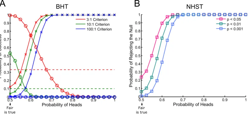
Now consider the probability of success for our experiments over a range of P(H) values from truly fair, P(H) =0.5, to completely biased, P(H) =1. Here we look at a more limited range of sample sizes from 20 to 200 and present results for all three criteria (see Figure 7A). As in Figure 6A, the bounds hold when the null hypothesis generated the data. However, when the null hypothesis is false, the experimenter favoring the null hypothesis can find substantial evidence (3:1) in support of the null in excess of the universal bound with coins that have a bias of up to
P(H) =0.7. For comparison, we also provide comparable p-values in Figure 7B. Again, we can see that when the null hypothesis generated the data, the probabilities of success exceed the true p-values. For slightly biased coins the number of trials is not large enough for either BHT or NHST to often find evidence that the coin is biased.
Though the results again show violations of expectations based on the universal bound, they also demonstrate another interesting property of BHT. Despite the apparent favorable outcome for the experimenter favoring the fair coin hypothesis when the coin is in fact fair, it can often take many trials before strong evidence can be found for the fair coin hypothesis. For example, Figure 7 shows that even the experimenter who preferentially supports the null hypothesis cannot find decisive evidence (100:1) within twenty to two hundred trials. Indeed, sometimes evidence for the fair coin hypothesis will lag behind evidence for the biased coin hypothesis. In Figure 6 when the coin is fair, it is possible to find strong evidence (10:1) for the biased coin within ten trials while it takes more than one hundred and fifty trials before strong evidence can be found for the fair coin hypothesis. This result comes about because until a large number of trials have been observed, there is no number of heads that produces strong evidence in favor of the fair coin hypothesis, while there are many possibilities (unlikely as they may be) that can produce strong evidence in favor of the biased coin hypothesis2.
2Johnson and Rossell (2010) note the slow accumulation of evidence for the null hypothesis and propose priors for the
Figure 7. The probability of successfully supporting either the fair coin or biased coin hypothesis with preferential stopping between the 20th and 200th trial. The fair coin hypothesis is only true ifP(H) =0.5. A) The probability of using BHT to successfully support the biased coin hypothesis (x) or support the fair coin hypothesis (o) given a specific true probability of heads and a specified Bayes factor threshold. The dashed lines are the universal bounds for each threshold. B) The probability of using NHST to successfully support the biased coin (squares) given a specific true probability of heads and a specified NHST threshold.
Bayesian t-tests
We now extend the results of fair and biased coins to the more practically relevant case of the t-test. The t-test is a basic statistical tool in psychology and is one of the first inferential methods taught to psychology students. As an alternative to the NHST t-test, a default Bayesian t-test has been developed by Rouder et al. (2009), and has recently been put in practice to compute Bayes factors for a wide range of previously published studies in psychology (Wetzels et al., 2011). This Bayesian t-test uses the same null hypothesis as the NHST t-test, an effect size of zero (δ=0), but
instead of merely specifying a non-zero effect size (δ6=0) as the composite alternative hypothesis,
a prior distribution is placed on the possible effect sizes. This allows researchers to compare the relative evidence for the alternative hypothesis against the null hypothesis and, unlike for NHST, allows researchers to quantify support for the null hypothesis using Bayes factors.
To investigate the consequences for preferential stopping for this case, we again assume two experimenters, one interested in finding support for the null hypothesis and the other interested in finding support for the alternative hypothesis. We assume the experimenters take a reasonable number of sequential samples (from 20 to 200) from a population with a particular mean,µ, and standard deviation equal to one, such that the effect size,δ, is equal to the mean,µ. Then we compute
the Bayes factor using the Bayesian t-test (Equation 1 from Rouder et al. (2009)). Experimenters stop if after any sample the Bayes factor exceeds their preferred criterion threshold.
considered a ’small’ effect size,δ=0.5 is a ’medium’ effect size, andδ=0.8 is a ’large’ effect size (Cohen, 1988). These labels ground the results of the simulations so that the probabilities of success can be associated with psychological effects for which the effect sizes are known. The same pattern of results was found as in the fair versus biased coin example; evidence for the alternative gradually increases with effect size, but reassuringly lies below the universal bounds when the null hypothesis generated the data (see Figure 8A).
This is an interesting result, both because it demonstrates where the probability of success appears bounded for BHT but not for NHST and also because the null hypothesis is not simple as it was in the fair coin case. Instead it is a particular kind of composite hypothesis, known as a point hypothesis, which fixes the effect size but allows the standard deviation to vary. This point null hypothesis becomes very similar to the simple hypothesis that generated the data after a number of trials because the point null hypothesis is a t distribution, which after a few hundred trials will be hard to distinguish from the data-generating Gaussian distribution. Here this unknown parameter has little effect – evidence against the null hypothesis remains below expectations based on the universal bound.
Once again, however, asδrises above 0, the results in Figure 8A indicate that evidence for
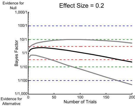
the null hypothesis can be above expectations based on the universal bound even when the effect size is non-zero. The probability of rejecting the null hypothesis using NHST is shown in Figure 8B as a comparison. We can also observe the non-monotonic mean path of Bayes factor in Figure 9, which shows how with a small effect size the Bayes factor initially favors the null hypothesis and later begins to favor the alternative hypothesis, an effect we explain in the next section and in the discussion.
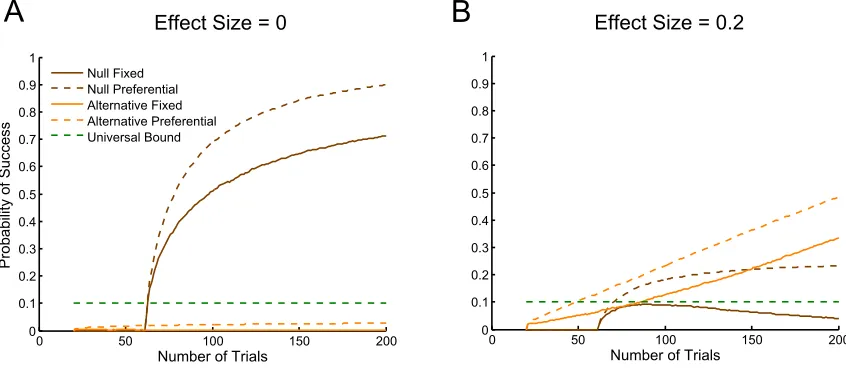
Figure 10 compares fixed and preferential stopping for data generated from the null hypothe-sis,δ=0, and using small effect sizes,δ=0.2, echoing the results of Figure 6. For a data generated
from the null hypothesis (Figure 10A), BHT is well behaved, with the caveat that more than fifty trials are needed before strong evidence for the null hypothesis can be found. The probability of generating strong evidence for the alternative hypothesis, even with preferential stopping, is below the values given by the universal bound. In contrast, when the effect size is small (Figure 10B), pref-erential stopping again influences the likelihood of an experimenter’s success beyond what would be expected if the universal bound applied.
Bounds on Generating Evidence When the Truth is Part of a Composite Hypothesis
Figure 8. The probability of successfully supporting either the null or alternative hypothesis with preferential stopping between the 20th and 200th trial. The null hypothesis is an effect size of zero (δ=0). A) The
probability of using the Bayesian t-test to successfully support the alternative hypothesis (x) or support the null hypothesis (o) given a specific data generating effect size and a specified Bayes factor threshold. The dashed lines are the universal bounds for each threshold. B) The probability of using NHST to successfully support the alternative hypothesis (squares) given a specific data generating effect size and a specified NHST threshold.
0 50 100 150 200
NumberdofdTrials
BayesdFactor
1/1,000 1/100 1/10 1/1 10/1 100/1 1,000/1
EffectdSized=d0.2
Evidencedfor Null
Evidencedford Alternative
[image:19.612.191.419.419.598.2]Figure 10. The probability of successfully using preferential stopping to support a hypothesis as the number of trials increases from 20 to 200 using a Bayes factor threshold of strong evidence (10:1). For the fixed stopping rule, the threshold is only checked at that particular trial number. For the preferential stopping rule, the probability of success is the proportion of experiments that have reached the threshold in favor of the preferred hypothesis at that particular trial or earlier. The dashed green represents the universal bound for the criterion. A) The true effect size is zero (the data were generated from the null hypothesis). B) the true effect size isδ=0.2 (the data were generated from a component of the alternative hypothesis).
and Seidenfeld (1996)) probability3. Helpfully, bounds on extensions to the fair and biased coins case have been proposed by Good (1967).
There are a couple arguments that have been put forward defending the intermediate favoring of the null hypothesis. The first is that researchers should not worry because the effect would have to so small as to have no practical relevance. For example, A. Smith and Spiegelhalter (1980) claimed that this behavior was not a problem because it would not have much of an effect on prediction4. We argue that the level of concern about the Bayesian t-test’s treatment of small effect sizes should de-pend on the implications of the hypotheses being tested. For hypotheses that are mainly of practical interest, such as whether a particular type of therapy is effective, small effect sizes are likely of little utility and methods that favor the null hypothesis should not be worrisome. However, some effects are of theoretical importance even if they are small. To take a recent extreme example, evidence that people could predict the future (Bem, 2011) would be interesting even if it only affected one in a billion trials. Though such a small effect would not be of practical use, it would still impact our understanding of not just psychology but also of biology and physics (Wagenmakers, Wetzels, Borsboom, & Maas, 2011). The second argument appeals to Occam’s razor, stating that simpler hypotheses should be favored when the data are weak and more complex hypotheses only if the
3Note that this holds to a lesser degree if the null hypothesis was not a point prior on an effect size of zero, instead
covering a range of possibilities that are narrower than the alternative. This is because the shrinking width of the likelihood with larger numbers of trials would exclude values that are probable under the null hypothesis as well. The point prior has been criticized (Cohen, 1994; Nester, 1996) and an alternative has been developed by Morey and Rouder (2011).
4More recent work has shown how prediction accuracy can be better maximized in this sort of situation (van Erven,
data are strong (Rouder et al., 2009). This argument has wider applicability and is reviewed in the discussion.
Finally, we note that in a particular sense the universal bound can apply to composite hy-potheses. In some situations, prior distributions can be constructed so that the prior probability on the parameters reflects the long run frequencies of these values occurring (Cox & Hinkley, 1974). For example, in psychology, it may be possible to construct a distribution of how often effect sizes of various magnitudes have occurred to use as the prior for the alternative hypothesis in a Bayesian t-test. We show in Appendix A that for such a composite hypotheses, the universal bound holds on average across experiments for these types of prior distributions. As an example, assume that a very thorough researcher interested in the reliability of an effect decided to replicate a variety of pub-lished studies that differ from one another, and replicated each of these studies many times. Assume as well that this researcher uses the distribution of effect sizes across these published experiments (and assuming the effect sizes are all perfectly estimated) as the prior of his alternative hypothesis in a Bayesian t-test. If the researcher examines only the set of replications of a single study, then the universal bound will not necessarily hold. However, on average across the entire set of replications of different types of materials, the universal bound will hold. There is no equivalent guarantee for NHST.
Discussion
We have shown that there are two common cases in psychological research for which the probabilities of finding convincing Bayes factors violate expectations based on the universal bound. These are 1) where the true hypothesis is not among the proposed hypotheses and 2) where a more general ‘composite’ hypothesis is true but the data lie close to the more constrained hypothesis. In both cases even fixed stopping can produce Bayes factors with probabilities greater than those given by the universal bound. Optional stopping, and particularly preferential stopping, can be used to further influence these frequencies. Though previous work has noted that the universal bound does not apply to composite hypotheses–e.g., in statistics (Mayo & Kruse, 2001; Royall, 2000, Rejoinder)–and the initial favoring of the null hypothesis in Bayes factors has been noted before in psychology and statistics (Atkinson, 1978; Matthews, 2011; Rouder et al., 2009), the work presented here provides a more thorough and general investigation of these findings, showing explicitly how they are related to violations of the assumptions of the universal bound. In particular, the present work demonstrates how large the influence of the choice of stopping rule can be.
Real Bayesians Don’t Need Frequentist Guarantees...
For Bayesians, Bayes factors represent nothing more than the relative likelihood of one hy-pothesis over another with respect to a particular set of data. Bayes factors obey the Likelihood Prin-ciple (Berger & Wolpert, 1988), meaning that they depend only on the data that have been actually observed rather than unobserved data, as frequentist methods do. Following from the Likelihood Principle is the Stopping Rule Principle: no matter what stopping rule is used by the experimenter, the relative evidence for the hypotheses (summarized by the Bayes factor) remains unchanged5 (Berger & Wolpert, 1988; Bernardo & Smith, 1994; Good, 1982; Jaynes, 2003; O’Hagan & Forster, 2004; Lindley, 1957). The is because Bayes factors are conditioned directly on the data and the data already tell us what the Bayes factor was at the time the experiment was stopped.
Even when the universal bound does not apply, the Bayes factors are correct. No modifica-tion should be made even if the experimenter used preferential stopping. Take, for example, the case in which neither hypothesis is true, such that the prior distribution over hypotheses gives zero weight to the process that generated the data. The Bayes factor still correctly describes the relative evidence for each of the hypotheses considered, whether or not the data generating hypothesis is also considered. The same is true for cases involving composite hypotheses. Furthermore, if the priors used match the beliefs of the researcher, then the initial favoring of the null hypothesis for small effect sizes is a feature, not a bug. As pointed out in Rouder et al. (2009), this initial favoring of the null hypothesis is an application of Occam’s razor – more data needs to be added into the same analysis for the more general alternative hypothesis to be supported. Comfortingly, enough data will eventually overcome most prior beliefs; consistency means that the best hypothesis will eventually win out.
...But It is Hard in Practice to Ignore Frequentist Implications
Despite the stopping rule being irrelevant to the interpretation of the evidence provided by Bayes factors, researchers may still not feel comfortable with the frequentist implications of the stopping rule choice. Academic researchers are rewarded by publishing, and publication is often based on whether theoretically interesting results are obtained. If the stopping rule used–whether fixed at a certain number of trials or preferential–can greatly change the magnitude or even the direction of the Bayes factors produced, then there is scope for experimenters to produce the ev-idence for which they would be most rewarded even if it contradicts the nature of the underlying phenomenon.
To illustrate, take the case of the Bayesian t-test and assume that we have a new, theoretically relevant, experimental paradigm in which the effect size, unknown to the experimenter, happens to be small. Now assume that the experimenter uses a default prior distribution on the alternative hypothesis that is fairly broad. If the experimenter believed that preferential stopping was irrelevant, then he may–as a result of theoretical motivations–pursue strong evidence for the null hypothesis with the consequence that he would have a good chance of finding it (as shown in Figure 8). In addition, onlookers may well also use broad priors to reflect their uncertainty and would interpret the results as strong evidence in favor of the null hypothesis, even if the experimenter revealed their
5The exception is for cases in which the stopping rule tells you something about the hypothesis that is not available
stopping rule (further results about onlookers are discussed in Kadane et al., 1996). An unprincipled experimenter has an even larger scope for affecting the results. If an unprincipled experimenter knew that the effect size in a paradigm was small, through either pilot experiments or extensive reading, he could design a study to change the beliefs of more na¨ıve onlookers in the direction he wished.
Fortunately there are some defenses against inadvertent or unprincipled use of stopping rules to change beliefs. The most broadly applicable is for reviewers to insist on a robustness analysis (Berger, 1993; Gallistel, 2009; Wagenmakers et al., 2011, Online Appendix). An investigation of the effects of a range of prior distributions on the resulting Bayes factors can provide a sense of how robust the results are to changes in the prior distribution. Using a narrower prior for an alternative hypothesis can make it more difficult to achieve convincing Bayes factors for the null hypothesis through optional stopping, though at the expense of requiring more trials to produce convincing evidence when the null hypothesis is correct. Another pre-emptive defense could be implemented by the experimenter. If the experimenter carefully chooses the stopping rule, then the frequentist properties of an experiment can be controlled (Berger, Brown, & Wolpert, 1994; Berger, Boukai, & Wang, 1997, 1999; Yu et al., submitted). A final defense is the interest of other researchers in the field who simply collect more data using a paradigm – the posterior distribution on effect sizes from the first experiment should then be used as the prior distribution for the new experiment, and with enough data the best hypothesis will be favored.
The first case we introduced where the universal bound does not hold, in which the data generating hypothesis is a combination of the hypotheses under consideration, presents additional problems for preventing experimenters from using stopping rules to produce evidence that suits them. In our first case, the prior distribution has no weight placed on the true generating model. An experimenter, who was either unaware that there was a heterogeneous population or aware but unprincipled, could test pure hypotheses and could, given some luck, use preferential stopping to produce their desired results. Here the issue is not uncertainty in the prior, which can be addressed by a robustness analysis, but that the prior puts no weight on the generating model. Fortunately, re-viewers in psychology have a strong tendency to ask whether results hold up at an individual partic-ipant level, which would prevent between-particpartic-ipant heterogeneity from being an issue. However, intra-individual heterogeneity or data generated from an integrated combination of the hypotheses remain problematic. These situations can be addressed somewhat by measures of model adequacy (Gelman, Meng, & Stern, 1996; Rubin, 1984), but they represent a real problem for any statistical approach and deserve further study.
Conclusions
frequentist properties of Bayes factors are dependent on optional stopping and where they are not, and that these properties could have practical implications for users of BHT. We hope this work highlights these potential problems and provides researchers with useful suggestions for how these frequentist implications can be controlled.
References
Armitage, P. (1960). Sequential medical trials. Springfield, IL: Thomas.
Armitage, P., McPherson, C. K., & Rowe, B. C. (1969). Repeated significance tests on accumulating data.
Journal of the Royal Statistical Society. Series A (General),132, 235-244.
Atkinson, A. C. (1978). Posterior probabilities for choosing a regression model.Biometrika,65, 39-48. Averell, L., & Heathcote, A. (2011). The form of the forgetting curve and the fate of memories. Journal of
Mathematical Psychology,55, 25-35.
Bartlema, A., Lee, M., Wetzels, R., & Vanpaemel, W. (submitted). Bayesian hierarchical mixture models of individual differences in selective attention and representation in category learning.
Bem, D. J. (2011). Feeling the future: experimental evidence for anomalous retroactive influences on cognition and affect.Journal of Personality and Social Psychology,100, 407-425.
Berger, J. O. (1993). An overview of robust Bayesian analysis. Test,3, 5-124.
Berger, J. O., Boukai, B., & Wang, Y. (1997). Unified frequentist and Bayesian testing of a precise hypothesis.
Statistical Science,12, 133-160.
Berger, J. O., Boukai, B., & Wang, Y. (1999). Simultaneous Bayesian-frequentist sequential testing of nested hypotheses.Biometrika,86, 79-92.
Berger, J. O., Brown, L. D., & Wolpert, R. L. (1994). A unified conditional frequentist and Bayesian test for fixed sequential simple hypothesis testing.The Annals of Statistics,22, 1787-1807.
Berger, J. O., & Wolpert, R. L. (1988). The likelihood principle.Institute of Mathematical Statistics. Bernardo, J. M., & Smith, A. F. M. (1994). Bayesian theory. New York: Wiley.
Birnbaum, A. (1962). On the foundations of statistical inference. Journal of the American Statistical Association,57, 269-306.
Breiman, L., LeCam, L., & Schwartz, L. (1964). Consistent estimates and zero-one sets. The Annals of Mathematical Statistics,35(1), 157–161.
Cohen, J. (1988).Statistical power analysis for the behavioral sciences. New York: Academic Press. Cohen, J. (1994). The earth is round (p< .05).American Psychologist,49, 997-1003.
Cox, D. R., & Hinkley, D. V. (1974). Theoretical statistics. London: Chapman and Hall.
Diaconis, P., & Freedman, D. (1986). On the consistency of bayes estimates.The Annals of Statistics, 1–26. Doob, J. L. (1949). Application of the theory of martingales. Le calcul des probabilites et ses applications,
23–27.
Ebbinghaus, H. (1974).Memory: A contribution to experimental psychology.New York: Dover.
Edwards, W., Lindman, H., & Savage, L. J. (1963). Bayesian statistical inference for psychological research.
Psychological Review,70, 193-242.
Fantino, E., Kulik, J., Stolarz-Fantino, S., & Wright, W. (1997). The conjunction fallacy: A test of averaging hypotheses.Psychonomic Bulletin & Review,4, 96–101.
Feller, W. (1968). An introduction to probability theory and its applications. New York: Wiley.
Francis, G. (2012). Too good to be true: Publication bias in two prominent studies from experimental psychology.Psychonomic Bulletin & Review,19, 151-156.
Gallistel, C. R. (2009). The importance of proving the null.Psychological Review,116, 439-453.
Gelman, A., Meng, X.-L., & Stern, H. (1996). Posterior predictive assessment of model fitness via realized discrepancies. Statistica Sinica,6, 733-807.
Gigerenzer, G., & Todd, P. M. (1999). Simple heuristics that make us smart. Oxford: Oxford University Press.
Good, I. J. (1982). Lindley’s paradox: Comment. Journal of the American Statistical Association, 77, 342-344.
Hacking, I. (1965).Logic of statistical inference. New York: Cambridge University Press.
Jarvstad, A., & Hahn, U. (2011). Source reliability and the conjunction fallacy. Cognitive Science,35, 682-711.
Jaynes, E. T. (2003).Probability theory: The logic of science. Cambridge: Cambridge University Press. Jeffreys, H. (1961).Theory of probability. Oxford: Oxford University Press.
Jennison, C., & Turnbull, B. (1990). Statistical approaches to interim monitoring of medical trials: a review and commentary.Statistical Science,5, 299-317.
John, L. K., Loewenstein, G., & Prelec, D. (2012). Measuring the prevalence of questionable research practices with incentives for truth telling.Psychological Science,23, 524-532.
Johnson, V. E., & Rossell, D. (2010). On the use of non-local prior densities in Bayesian hypothesis tests.
Journal of the Royal Statistical Society: Series B (Statistical Methodology),72, 143-170.
Kadane, J. B., Schervish, M. J., & Seidenfeld, T. (1996). When several Bayesians agree that there will be no reasoning to a foregone conclusion.Philosophy of Science,63, 281-289.
Kass, R. E., & Rafferty, A. E. (1995). Bayes factors. Journal of the American Statistical Association,90, 773-795.
Kerridge, D. (1963). Bounds for the frequency of misleading Bayes inferences.The Annals of Mathematical Statistics,34, 11091110.
Kruschke, J. K. (2010). What to believe: Bayesian methods for data analysis. Trends in Cognitive Sciences,
14, 293-300.
Lee, M. D. (2011). How cognitive modeling can benefit from hierarchical Bayesian models. Journal of Mathematical Psychology,55, 1-7.
Lee, M. D., & Cummins, T. D. R. (2004). Evidence accumulation in decision making: Unifying the “take the best” and the “rational” models. Psychonomic Bulletin & Review,11, 343-352.
Lewis, S., & Raftery, A. E. (1997). Estimating Bayes factors via posterior simulation with the Laplace-Metropolis estimator.Journal of the American Statistical Association,92, 648-655.
Lindley, D. (1957). A statistical paradox. Biometrika,44, 187-192.
Matthews, W. J. (2011). What might judgment and decision making research be like if we took a Bayesian approach to hypothesis testing? Judgment and Decision Making,6, 843-856.
Mayo, D. G., & Kruse, M. (2001). Principles of inference and their consequences. In D. Cornfield & J. Williamson (Eds.),Foundations of bayesianism(p. 381-403). Dordrecht: Kluwer Academic Pub-lishers.
Medin, D. L., & Schaffer, M. M. (1978). Context theory of classification learning. Psychological Review,
85, 207-238.
Morey, R. D., & Rouder, J. N. (2011). Bayes factor approaches for testing interval null hypotheses. Psycho-logical Methods,16, 406-419.
Nester, M. R. (1996). An applied statistician’s creed. Applied Statistics,45, 401-410.
Nilsson, H., Winman, A., Juslin, P., & Hansson, G. (2009). Linda is not a bearded lady: configural weighting and adding as the cause of extension errors. Journal of Experimental Psychology: General, 138, 517-534.
Nosofsky, R. M. (1986). Attention, similarity, and the identification-categorization relationship. Journal of Experimental Psychology: General,115, 39-57.
O’Hagan, A., & Forster, J. (2004).Bayesian inference(2nd edition ed., Vol. 2B). London: Arnold. Pocock, S. J. (1983).Clinical trials: A practical approach. Wiley-Blackwell.
Reed, S. K. (1972). Pattern recognition and categorization.Cognitive Psychology,3, 393-407.
Rieskamp, J., & Hoffrage, U. (2008). Inferences under time pressure: How opportunity costs affect strategy selection.Acta Psychologica,127, 258-276.
Rouder, J. N., Speckman, P. L., Sun, D., Morey, R. D., & Iverson, G. (2009). Bayesian t-tests for accepting and rejecting the null hypothesis.Psychonomic Bulletin & Review,16, 225-237.
Royall, R. (1997).Statistical evidence: A likelihood paradigm. London: Chapman & Hall.
Royall, R. (2000). On the probability of observing misleading statistical evidence (with discussion).Journal of the American Statistical Association,95, 760-768.
Rubin, D. B. (1984). Bayesianly justifiable and relevant frequency calculations for the applied statistician.
The Annals of Statistics,12, 1151-1172.
Smith, A., & Spiegelhalter, D. J. (1980). Bayes factors and choice criteria for linear models. Journal of the Royal Statistical Society. Series B (Methodological),42, 213-220.
Smith, C. (1953). The detection of linkage in human genetics.Journal of the Royal Statistical Society. Series B,15, 153-192.
van Erven, T., Gr¨unwald, P., & de Rooij, S. (2012). Catching up faster by switching sooner: A predictive approach to adaptive estimation with an application to the AIC–BIC dilemma. Journal of the Royal Statistical Society B,74, 361–417.
Wagenmakers, E.-J. (2007). A practical solution to the pervasive problems of p values.Psychonomic Bulletin & Review,14, 779-804.
Wagenmakers, E.-J., Lodewyckx, T., Kuriyal, H., & Grasman, R. (2010). Bayesian hypothesis testing for psychologists: a tutorial on the Savage-Dickey method.Cognitive Psychology,60, 158-189.
Wagenmakers, E.-J., Wetzels, R., Borsboom, D., & Maas, H. L. J. van der. (2011). Why psychologists must change the way they analyze their data: the case of psi: Comment on Bem (2011). Journal of Personality and Social Psychology,100, 426-432.
Wald, A. (1947). Sequential analysis. New York: Wiley.
Wetzels, R., Matzke, D., Lee, M. D., Rouder, J. N., Iverson, G. J., & Wagenmakers, E.-J. (2011). Statistical evidence in experimental psychology: An empirical comparison using 855 t tests. Perspectives on Psychological Science,6, 1-15.
Wixted, J. T., & Ebbesen, E. B. (1991). On the form of forgetting.Psychological Science,2, 409-415. Wyer, R. S. (1976). An investigation of the relations among probability estimates. Organizational Behavior
and Human Performance,15, 1-18.
Yu, E. C., Sprenger, A. M., Thomas, R. P., & Dougherty, M. R. (submitted). When decision heuristics and science collide.
Appendix A: Proofs of the Universal Bound and Its Exceptions
The universal bound has been noted by many authors (e.g., Birnbaum, 1962; C. Smith, 1953). The claim is that the probability of observing data that produce a likelihood ratio ofkin favor of a false hypothesis is less than or equal to 1/k. Here we give a proof following C. Smith (1953). The first step of this proof is to calculate the expected value of the likelihood ratio over all possible data. LetT be the simple true hypothesis andFthe simple false hypothesis.
ET
P(Xn|F)
P(Xn|T)
=
∑
Xn
P(Xn|F)
P(Xn|T)
P(Xn|T) =
∑
XnP(Xn|F) =1 (9)
whereET indicates taking the expected value over the probability of each data set given the true hypothesis – the first equality is the expected value written explicitly. The third equality holds because the total probability of all the possible data under any probability distribution is one.