Development of nuclear magnetic resonance methods for determination of membrane protein structure

University of Warwick institutional repository:

http://go.warwick.ac.uk/wrap

A Thesis Submitted for the Degree of PhD at the University of Warwick

http://go.warwick.ac.uk/wrap/56857

This thesis is made available online and is protected by original copyright.

Please scroll down to view the document itself.

Magnetic Resonance Methods

for Determination of Membrane

Protein Structure

Dharmesh K. Patel

A thesis submitted in partial fulfilment of the requirements

for the degree of Doctor of Philosophy

Department of Chemistry

P a g e| i

i.

TABLE OF CONTENTS

i. Table of contents ... i

ii. List of figures ... vii

iii. List of tables ... xi

iv. Acknowledgments ... xii

v. Declaration... xiii

vi. Abbreviations ... xiv

vii. Summary ... xx

1

INTRODUCTION ... 1

1.1 Membrane proteins ... 1

1.1.1 Challenges when studying membrane proteins ... 2

1.1.2 Expression ... 2

1.1.3 Solubilisation... 4

1.1.4 Purification ... 5

1.2 Membrane mimetic systems ... 6

1.2.1 Detergent micelles ... 7

1.2.2 Liposomes ... 7

1.2.3 Amphipols and nanodiscs ... 9

1.2.4 Bicelles ... 10

1.3 Methods for structure determination ... 12

1.3.1 X-ray crystallography ... 12

1.3.2 Solution NMR ... 13

P a g e| ii

1.3.4 Chemical shift anisotropy (CSA) ... 15

1.3.5 Dipolar coupling ... 15

1.3.6 Quadrupolar coupling ... 16

1.4 NMR Theory ... 17

1.4.1 Spin ... 17

1.4.2 Magnetisation ... 19

1.4.3 R.F pulses and the Rotating Frame ... 21

1.4.4 Chemical Shift ... 23

1.4.5 Two dimensional (2D) NMR ...24

1.5 Solid state NMR ... 26

1.5.1 Magic angle spinning (MAS) ... 27

1.5.2 Cross polarisation (CP) ... 28

1.5.3 Proton decoupling ... 29

1.5.4 Recoupling ... 30

1.5.5 Dipolar Assisted Rotational Recoupling (DARR) ... 30

1.6 Glycophorin A (GpA) as a model TM ... 32

1.7 Bovine Papillomavirus E5 (BPV E5) ... 33

1.8 Aims and objectives of this study ... 35

1.9 References ... 36

2

MATERIALS AND METHODS ... 41

2.1 Reagents and Chemicals ... 41

2.2 Buffers... 41

2.3 Peptide design ...42

2.3.1 Glycophorin A (GpA) peptides ...42

P a g e| iii

2.4 Peptide purification using reverse-phase high performance liquid chromatography

43

2.5 Mass Spectrometry ...45

2.5.1 Electrospray Ionisation (ESI) Mass spectrometry ...45

2.5.2 Matrix Assisted Laser desorption Ionisation (MALDI) Mass spectrometry ...45

2.6 Peptide preparation and characterisation ...46

2.6.1 Lyophilisation ...46

2.6.2 Protein concentration determination ...46

2.6.3 SDS-PAGE analysis of purified peptides ...47

2.6.4 Coomassie staining ...47

2.6.5 Silver staining ...47

2.7 Peptide reconstitution into lipid vesicles ...48

2.7.1 Detergent solubilisation of peptides ...48

2.7.2 Detergent removal ...49

2.7.3 Co-solubilisation ... 50

2.7.4 Transfer of samples to solid state NMR rotor ... 51

2.8 Characterisation of proteoliposomes ... 51

2.8.1 Circular Dichroism (CD) spectroscopy ... 51

2.8.2 Attenuated Total Reflection Fourier Transform Infrared (ATR-FTIR) spectroscopy 52 2.8.3 Electron Microscopy (EM) ... 53

2.9 Magic Angle Spinning (MAS) Solid state NMR spectroscopy ...54

2.9.1 Solid state NMR experimental procedure ...54

2.9.2 1D 31_P/1_{H lipid NMR experiments ... 55}

P a g e| iv

2.9.4 2D 13_C-13_{C DARR NMR experiments ... 56}

2.9.5 2D 13_C-15_{N NMR experiments ... 56}

2.10 Solution NMR experiments ... 57

2.10.1 Bicelle preparation ... 57

2.10.2 Solution NMR experimental procedure... 58

2.10.3 1D 1_{H NMR spectroscopy ... 58}

2.10.4 2D heteronuclear NMR spectroscopy ... 58

2.10.5 3D heteronuclear NMR spectroscopy ... 59

2.11 References ... 59

3

PEPTIDE DESIGN, PREPARATION AND CHARACTERISATION ...

62

3.1 Introduction ... 62

3.2 Peptide design and purification for ssNMR analyses ... 63

3.3 Reconstitution of GpA peptide into lipid vesicles ... 75

3.3.1 CD for screening of detergents ... 76

3.3.2 Electron Microscopy ... 81

3.3.3 ATR-FTIR analysis of reconstituted peptides ... 83

3.3.4 Co-solubilisation of E5 peptides ... 87

3.4 Summary ... 90

3.5 References ... 92

4

SOLID STATE NMR ANALYSIS OF RECONSTITUTED GPA ... 94

4.1 Introduction ...94

4.2 13_{C NMR of doubly labelled GpA} VG peptide reconstituted using the detergent removal method ... 95

4.2.1 1D 13_{C ssNMR spectra of doubly labelled (GpA} VG) peptide ... 96

P a g e| v

4.2.3 1D 13_{C ssNMR of GpA}

VG prepared using the co-solubilisation method ... 104

4.2.4 2D 13_C-13_{C DARR ssNMR ... 106}

4.2.5 Relating cross peaks observed to existing GpA structure ... 111

4.3 Alternative peptide labelling scheme. ... 113

4.3.1 ssNMR of singly labelled GpA peptides. ... 115

4.3.2 Singly labelled GpA build-up curves ... 118

4.4 15_{N GpA ssNMR ... 121}

4.4.1 1D 15_{N ssNMR of singly labelled GpA sample ... 121}

4.4.2 2D 15_N-13_{C ssNMR of singly labelled GpA sample... 123}

4.5 Summary ... 129

4.6 References ... 131

5

SOLID STATE NMR ANALYSIS OF BPV E5 ... 133

5.1 Introduction ... 133

5.2 1D 13_{C ssNMR of BPV E5 labelled at leucine and phenylalanine (BPV E5} LF) ... 134

5.2.1 2D 13_C-13_{C ssNMR of BPV E5} LF ... 139

5.3 1D 13_{C ssNMR of BPV E5 labelled at tyrosine and phenylalanine (BPV E5} FY) ... 144

5.3.1 Optimisation of experimental parameters in 1D CP experiments ... 149

5.3.2 Optimisation of experimental parameters: temperature ... 150

5.3.3 Optimisation of experimental parameters: contact time ... 153

5.3.4 2D 13_C-13_{C ssNMR of BPV E5 labelled at phenylalanine & tyrosine (BPV E5} FY) ... 156

5.4 ssNMR characterisation of DMPC/cholesterol lipid membranes ... 160

5.4.1 Characterisation of lipid membranes by static 31_{P ssNMR ... 160}

5.4.2 Characterisation of lipid membranes by 1_{H MAS ssNMR ... 165}

5.5 Summary ... 170

P a g e| vi

6

SOLUTION NMR ANALYSIS OF BPV E5 ... 175

6.1 Introduction ... 175

6.2 Solution NMR analysis of BPV E5V2 ... 178

6.2.1 Solution NMR analysis of BPV E5V2 in TFE... 179

6.3 Solution NMR analysis of BPV E5V2 in bicelles... 182

6.3.1 Solution NMR of BPV E5V2 in q=0.33 bicelles. ... 186

6.3.2 3D HSQC TOCSY and NOESY analysis of BPV E5V2 ... 188

6.4 Solution NMR analysis of BPV E5LF in bicelles ... 195

6.5 Characterisation of DMPC/DHPC bicelles ... 197

6.5.1 Analysis of bicelles by 31_{P solution NMR ... 198}

6.5.2 Analysis of bicelles by DLS ... 199

6.6 Summary ... 201

6.7 References ... 204

7

206

7.1 Discussion ... 206

P a g e| vii

ii.

LIST OF FIGURES

Figure 1.1 Cartoon representation of a detergent micelle ... 4

Figure 1.2 Schematic representation of a nanodisc ... 10

Figure 1.3 Cartoon representation of a bicelle. ... 12

Figure 1.4 Single spin angular magnetic moment ... 17

Figure 1.5 Zeeman splitting of energy levels ... 19

Figure 1.6 Orientation and precession of nuclear spins ... 20

Figure 1.7 Magnetisation and rotating frame of reference ... 21

Figure 1.8 Free Induction Decay (FID) ... 23

Figure 1.9 2D NMR experiment. ... 25

Figure 1.10 Illustration of rotor assembly in a magic angle spinning experiment ... 27

Figure 1.11 Dipolar Assisted Rotational Resonance (DARR) pulse sequence. ... 31

Figure 1.12 Schematic of the magnetisation transfer within a protein in a DARR experiment. ... 31

Figure 1.13 Structural model of the Glycophorin A TM domain dimer ... 33

Figure 1.14 Peptide sequence encoded for by Type I BPV E5 gene ... 33

Figure 1.15 Schematic of the symmetrical model of the BPV E5 dimer ... 35

Figure 2.1 Schematic of ATR-FTIR setup ... 53

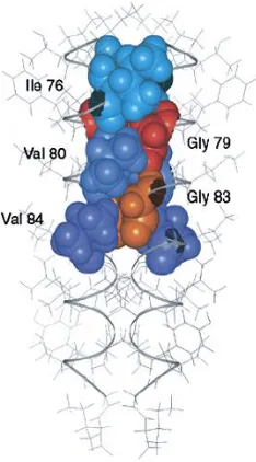
Figure 3.1 3D structure of the alpha-helical homodimer transmembrane Glycophorin A (GpA) ... 63

Figure 3.2 Ball and stick representation of the GpA homodimer interface ...64

Figure 3.3. Isotopically labelled GpA TM domain peptide sequences ... 65

Figure 3.4 Molecular model of BPV E5 transmembrane protein generated from CHI ... 66

Figure 3.5 Molecular model of selected E5 dimer interfacial regions generated using CHI ... 68

Figure 3.6 Isotopically labelled E5 TM domain peptide sequences ... 68

Figure 3.7 Representative RP-HPLC chromatogram of crude GpA purification ... 70

Figure 3.8 Representative RP-HPLC chromatogram of crude BPV E5 purification ... 70

Figure 3.9 RP-HPLC chromatogram of purified BPV E5 peptide ... 71

Figure 3.10 GpA Deconvoluted ESI-MicroTOF mass spectra ... 73

Figure 3.11 BPV E5 Deconvoluted ESI-MicroTOF mass spectra ...74

Figure 3.12 CD spectra of GpA peptide dissolved in TFE ... 78

Figure 3.13 CD spectra of GpA peptide dissolved in varying detergents ... 78

Figure 3.14 Secondary structure analysis of CD data ... 79

Figure 3.15 Overview of reconstitution protocols ... 80

Figure 3.16 Images obtained by TEM using negative staining ... 81

Figure 3.17 CD spectrum of GpA proteoliposome solutionobtained by Capillary CD ... 82

P a g e| viii

Figure 3.19 FTIR spectrum of the GpApeptide in DMPC liposomes containing 5% cholesterol

prepared using the detergent removal method ... 85 Figure 3.20 FTIR spectrum of the GpA peptide in DMPC liposomes containing 5% cholesterol prepared using the co-solubilisation method ... 86

Figure 3.21 1D 13_{C spectra obtained from samples prepared by detergent removal (blue) and}

co-solubilisation (red) ... 87

Figure 3.22 FTIR spectrum of the E5TM peptide in DMPC liposomes prepared using the

co-solubilisation method... 88 Figure 3.23 CD spectrum of BPV E5 proteoliposome solution prepared for solid state NMR using the co-solubilisation method ... 89 Figure 4.1 Chemical structure of valine and glycine. ... 96

Figure 4.2 1D proton-decoupled 13_{C CP-MAS spectrum of doubly labelled GpA}

VG in DMPC

liposomes prepared using the detergent removal method ... 97 Figure 4.3 1D proton-decoupled 13_{C CP-MAS spectrum of DMPC with 5% cholesterol ... 98}

Figure 4.4 Experimentally derived secondary chemical shifts for GpA ... 104

Figure 4.5 1D proton-decoupled 13_{C CP-MAS spectrum of doubly labelled GpA}

VG in DMPC

liposomes prepared using the co-solubilisation method. ... 105

Figure 4.6 20 ms 2D 13_C-13_{C DARR spectrum of doubly labelled GpA}

VG in DMPC liposomes.

... 107 Figure 4.7 Overlay of 20 & 400 ms 2D 13_C-13_{C DARR spectra of doubly labelled GpA}

VG in

DMPC liposomes. ... 108 Figure 4.8 Aliphatic regions of 2D 13_C-13_{C DARR spectra of doubly labelled GpA}

VG at short

and long mixing times. ... 110 Figure 4.9 Molecular model of human GpA homodimer ... 113 Figure 4.10 Diagrammatic form of alternative peptide labelling scheme ... 115 Figure 4.11 1D proton-decoupled 13_{C CP-MAS spectrum of singly labelled GpA}

V + GpAG

mixture in DMPC liposomes prepared using the co-solubilisation method ... 116

Figure 4.12 Overlaid 400 ms 2D 13_C-13_{C DARR correlation spectrum of doubly labelled GpA}

(GpAVG) vs. singly labelled GpAV + GpAG ... 118

Figure 4.13 Build-up curves for intra-residue and inter-residue GpA cross peaks ... 120 Figure 4.14 1D proton-decoupled 15_{N CP-MAS spectrum of singly labelled GpA in DMPC}

liposomes prepared using the co-solubilisation method ... 122 Figure 4.15 2D 15_N-13_{C TEDOR spectra of singly labelled GpA}

V + GpAG peptides in

DMPC/cholesterol liposomes ... 125 Figure 4.16 1D extracted rows from 2D 15_N-13_{C TEDOR spectra of valine resonances in singly}

labelled GpAV + GpAG peptides ... 126

Figure 4.17 1D extracted row from 2D 15_N-13_{C TEDOR spectra of glycine resonances in singly}

labelled GpAV + GpAG peptides ... 127

P a g e| ix

Figure 5.2 1D proton-decoupled 13_{C CP-MAS spectrum of singly labelled BPV E5}

LF in DMPC

liposomes ... 137 Figure 5.3 20 ms 2D 13_C-13_{C DARR spectrum of singly labelled BPV E5}

LF in DMPC liposomes.

... 140 Figure 5.4 400 ms 2D 13_C-13_{C DARR spectrum of singly labelled BPV E5}

LF in DMPC liposomes.

... 141 Figure 5.5 Overlay of 20 and 400 ms 2D 13_C-13_{C DARR spectra of singly labelled BPV E5}

LF in

DMPC liposomes. ... 142 Figure 5.6 Chemical structure of phenylalanine and tyrosine. ... 144

Figure 5.7 1D proton-decoupled 13_{C CP-MAS spectrum of singly labelled BPV E5}

FY in DMPC

liposomes ... 147

Figure 5.8 1D proton-decoupled 13_{C CP-MAS spectra of singly labelled BPV E5}

FY at

decreasing temperature ... 151 Figure 5.9 Average peak width of 13_{C BPV E5}

FY resonances as a function of temperature .... 152

Figure 5.10 1D proton-decoupled 13_{C CP-MAS spectra of singly labelled BPV E5} FY at

increasing CP contact time ... 154 Figure 5.11 Graph of 1D 13_{C resonance signal intensity at increasing cross polarisation (CP)}

contact times ... 155 Figure 5.12 50 ms 2D 13_C-13_{C DARR spectrum of singly labelled BPV E5}

YF in DMPC liposomes

... 157 Figure 5.15 400 ms 2D 13_C-13_{C DARR spectrum of singly labelled BPV E5}

YF in DMPC

liposomes ... 158 Figure 5.16 50 vs 400 ms 2D 13_C-13_{C DARR spectrum of singly labelled BPV E5}

YF in DMPC

liposomes ... 159 Figure 5.15 Lipid polymorph and phase behaviour ... 161 Figure 5.16 1D proton-decoupled static 31_{P spectra of DMPC liposomes with increasing}

cholesterol concentration at varying temperature ... 162 Figure 5.17 Variation of 31_{P chemical shift anisotropy of DMPC/cholesterol liposomes with}

temperature ... 164

Figure 5.18 1D 1_{H spectra of DMPC liposomes with increasing cholesterol concentration at}

varying temperature ... 165 Figure 5.19 Cartoon of cholesterol intercalating between lipid molecules at high and low temperatures... 169 Figure 6.1 Peptide sequence of 15_{N labelled BPV E5}

V2 peptide ... 178

Figure 6.2 Molecular model of BPV E5V2 homodimer with 15N labelled amino acids indicated

... 179 Figure 6.3 1D 1_{H spectrum of BPV E5}

V2 in deuterated TFE ... 180

Figure 6.4 2D 15_N-1_{H HSQC spectrum of BPV E5}

V2 in deuterated TFE ... 181

Figure 6.5 2D 15_{N –} 1_{H HSQC spectra of BPV E5}

V2 in DMPC/DHPC bicelles at increasing

P a g e| x Figure 6.6 Extracted planes from 2D 15_N-1_{H HSQC spectra at increasing temperatures ... 185}

Figure 6.7 Overlay of 2D 15_{N -} 1_{H HSQC of BPV E5}

V2 reconstituted into q=0.33 and q=0.5

bicelles ... 187 Figure 6.8 15_{N edited} 1_H-1_{H HSQC TOCSY of BPV E5}

V2 reconstituted into q=0.33 bicelles .. 190

Figure 6.9 15_{N edited} 1_H-1_{H NOESY-HSQC spectrum of BPV E5}

V2 reconstituted into q=0.33

bicelles ... 192 Figure 6.10 2D 15_{N -} 1_{H HSQC of BPV E5V2 reconstituted into q=0.33 bicelles with tentative}

amino acid assignments ... 193 Figure 6.11 2D 15_{N -} 1_{H HSQC of BPV E5}

LF reconstituted into q=0.25 bicelles ... 196

P a g e| xi

iii.

LIST OF TABLES

Table 2.1 List of isotopically labelled GpA peptides used in this study ...42

Table 2.2 List of isotopically labelled BPV E5 peptides used in this study ...43

Table 2.3 Gradient used for the purification of GpA peptides by RP-HPLC ... 44

Table 2.4 Gradient used for the purification of BPV E5 peptides by RP-HPLC ... 44

Table 2.5 List and properties of detergents used in this study ...49

Table 3.1 Table of the shortest inter-helical distance between amino acids at the E5 dimer interface... 67

Table 3.2 Summary of observed charge states for peptides used in this study analysed by ESI-MS ... 72

Table 4.1 List of previously assigned dimyristoyl-sn-phosphatidylcholine (DMPC) resonances ... 99

Table 4.2 13_{C chemical shift data for labelled GpA Val 80 and Gly 83... 100}

Table 4.3 13_{C chemical shift data for secondary species in labelled GpA Val 80 and Gly 83 .. 101}

Table 4.4 Comparison of experimental GpA chemical shifts compared to random coil values ... 103

Table 4.5 Average distances between valine 80 and glycine 83 carbon atoms in the published GpA homodimer structure ... 111

Table 4.6 15_{N chemical shift data for labelled GpA Val 80 and Gly 83 ... 122}

Table 4.7 13_{C line widths for GpA Val 80 and Gly 83 extracted from rows of 2D} 15_N-13_C z-filtered TEDOR experiments ... 128

Table 5.1 13_{C chemical shift data for labelled BPV E5 Leu 24 and Phe 28 ... 138}

Table 5.2 13_{C chemical shift data for labelled BPV E5 Phe 28 and Tyr 31 ... 149}

Table 5.3 1_{H chemical shift data for DMPC natural abundance lipid resonances ... 166}

Table 6.1 Chemical shift assignments for 15_{N labelled amino acids in BPV E5} V2 reconstituted in DMPC/DHPC bicelles ... 194

Table 6.2 Tentative chemical shift assignments for labelled BPV E5 Leu 24 and Phe 28 in bicelles ... 197

P a g e| xii

iv.

ACKNOWLEDGMENTS

ॐ

First and foremost I would like to thank my supervisor Ann Dixon, for giving me the opportunity to work on a project in a though and exciting field of science, her excellent supervision and guidance throughout this project and her input in the preparation of this manuscript have been invaluable. Not only has she been a brilliant supervisor, but also a great friend, someone who I could always go to talk to or share a laugh with and as such will I will always be indebted to her.

I would also like to thank Steven Brown for his input and suggestions in the direction of this study, his knowledge of the field has helped immensely. I would also like to thank Johanna-Becker Baldus, who taught me the many joys of setting up solid-state NMR experiments, Fredrik Romer and all other members of Solid state NMR group who have helped when things have gone wrong. My thanks also to my academic panel Peter Sadler and Pat Unwin for their input into my project and to Janet Crawford for synthesising the peptides used in this study.

I would also like to thank all members of the Dixon group, past and present for their helpful discussion (including Friday Pictionary), friendship and support throughout the four years that I have been here at Warwick, in particular Gemma Warren, Michael Chow, Fay Probert, Esther Martin for making researching towards a thesis enjoyable and especially Maria Tareen for all her help in proofreading and to print this manuscript. Many thanks to all my friends in Chemical Biology and the whole Chemistry department whom I have not named here. I would also like to thank Alison Rodger and the members of her group for the use of equipment and helpful discussion throughout my research.

P a g e| xiii

v.

DECLARATION

The work in this thesis is original, and was conducted by the author, unless otherwise stated, under the supervision of Dr Ann M. Dixon (Department of Chemistry) and in collaboration with Professor Steven Brown (Department of Physics).

It has not previously been presented for another degree.

Funding was provided by an EPSRC studentship.

All sources of information have been acknowledged by means of reference.

P a g e| xiv

vi.

ABBREVIATIONS

aa

Amino acids

ACN

Acetonitrile

AU

Absorbance units

ATR-FTIR

Attenuated total reflectance Fourier transform

infrared

spectroscopy

β-OG

β-Octyl glucoside

BMRB

Biological magnetic resonance databank

BPV

Bovine papilloma virus

CD

Circular dichroism

CHI

CNS searching of helix interactions

CMC

Critical micelle concentration

CP

Cross polarisation

CP MAS

Cross polarisation magic angle spinning

CSA

Chemical shift anisotropy

A

B

P a g e| xv

1D

one-dimensional

2D

two-dimensional

3D

three-dimensional

DARR

Dipolar assisted rotational recoupling

dH

O

Distilled water

DDM

Dodecylmaltoside

DHPC

1,2-Dihexanoyl-sn-glycero-3-phosphocholine

DLS

Dynamic light scattering

DMPC

1,2-Dimyristoyl-sn-glycero-3-phosphocholine

DPC

Dodcylphophocholine

EM

Electron microscopy

ESI-MS

Electrospray ionisation mass spectrometry

FT

Fourier transform

D

E

P a g e| xvi

g

Grams

GpA

Glycophorin A

HEPES

4-(2-hydroxyethyl)-1-piperazineethanesulfonic acid

HPLC

High performance liquid chromatography

hr

Hours

HSQC

Hetronuclear single quantum coherence

Hz

Hertz

IPA

Isopropanol

kDa

kilo Dalton

kHz

Kilo Hertz

L

Lamellar liquid crystalline phase

L

Lamellar gel phase

G

H

I

K

P a g e| xvii

L

Lamellar liquid ordered phase

LD

Linear dichroism

LPR

Lipid to protein ratio

MALDI-TOF

Matrix-assisted laser desorption ionisation time of flight

MAS

Magic angle spinning

mg

Milligram

MHz

Mega Hertz

mL

Millilitre

mM

Millimolar

ms

Millisecond

NMR

Nuclear magnetic resonance

nm

Nanometre

NOE

Nuclear Overhauser enhancement

NOESY

Nuclear Overhauser spectroscopy

M

P a g e| xviii

OCD

Oriented circular dichroism

OG

octyl-glucoside

ppm

Parts per million

REDOR

Rotational echo double resonance

RF

Radio frequency

RPM

Revolutions per minute

RT

Room temperature

SDS

Sodium dodecyl sulphate

ssNMR

Solid state NMR

T

Longitudinal relaxation time

T

Transversal relaxation time

TEDOR

Transferred echo double resonance

O

P

R

S

P a g e| xix

TFA

Trifluoroacetic acid

TFE

2,2,2-Trifluroethanol

TOCSY

Total correlation spectroscopy

TM

Transmembrane

TRIS

tris (hydroxymethyl) aminomethane

UV

Ultraviolet

w/v

Weight per volume

Greek symbols

ε

Extinction coefficient

λ

Wavelength

µg

Micro gram

µL

Micro litre

µM

Micro molar

U

P a g e| xx

vii.

SUMMARY

Membrane proteins represent over a third of all proteins encoded for by the human genome and play a vital role in the functionality of the cell, by controlling a vast number of cellular processes. With over half of pharmacological drugs targeting membrane proteins, their importance is not to be under estimated. Yet the number of three-dimensional membrane protein structures reported to date falls well short of that of their water soluble counterparts. This discrepancy can directly be attributed to the difficulties involved in studying membrane protein structure due to their hydrophobic nature, resulting in a number of challenges in the production and purification of protein, whilst requiring the use of a suitable membrane mimetic upon extraction from their native membrane.

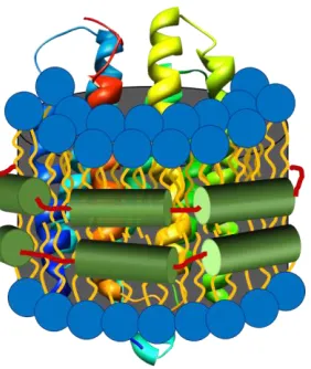
Solid state NMR (ssNMR) as a technique for studying membrane protein structure is well placed in being able to obtain structural information for membrane proteins in “native-like” lamellar bilayer environments but there are challenges involved in preparing suitable samples for analysis. As there is no “one suit fits all” method for preparing membrane protein samples for ssNMR analysis, conditions that result in fully reconstituted protein, that also allow for high resolution structural analysis have to be trialled.

This study presents work on sample preparation methods for the reconstitution of the small alpha helical transmembrane (TM) proteins, using the well characterised TM protein Glycophorin A (GpA) as a model peptide. Established biophysical and NMR techniques were used to characterise DMPC lipid embedded peptides prepared using two reconstitution techniques. The limited site specific labelling at key positions of the GpA homodimer was used to evaluate the feasibility of using similar sample preparation and labelling schemes when applied to that of the Bovine Papillomavirus E5 (BPV E5) TM protein, for which no solved three-dimensional structure exists. Characterisation of the DMPC membranes into which membrane proteins where reconstituted was also conducted. To compliment ssNMR analysis of BPV E5, preliminary work on the use of fast tumbling isotropic bicelles to study

P a g e| 1

1

INTRODUCTION

1.1

Membrane proteins

An integral part of a biological cell is the lipid membrane. In addition to sequestering the contents of the cell, the lipid membrane provides an interface through which the cell can interact with its external environment. The properties of the lipid membrane are influenced by membrane proteins which span across the lipid bilayer. Membrane proteins account for over 30% of the proteins expressed by the human genome (Wallin and von Heijne 1998) and play a vital role in controlling a vast number of cellular functions such as; cell signalling, signal transduction and the trafficking of molecules across the cell membrane. Membrane proteins therefore play a key role in the functionality of the cell and the organism as a whole, as defects in their function can be associated to many diseases and causes of tumorigenesis in eukaryotes (Sanders and Nagy 2000; Sanders and Myers 2004; Aperia 2007). It is for these reasons in particular that membrane proteins are of such significant interest due to their huge potential as pharmaceutical targets in the development of novel therapies against a range of diseases. Currently it is estimated that up to 50% of current drug pharmacological drugs target membrane proteins for their action (Russell and Eggleston 2000), with G-protein coupled receptors (GPCRs) representing the most popular membrane protein target (Russell and Eggleston 2000). Therefore obtaining structural information for membrane proteins is highly beneficial in characterising their functionality and towards designing more effective drugs that are more specific towards their membrane protein targets.

P a g e| 2 Despite their importance, the number of three-dimensional structures determined for membrane proteins to date remains relatively small when compared to that of soluble proteins, comprising less than one in a hundred structures that have been deposited in the Protein Data Bank (PDB) (www.pdb.org, (Berman, Westbrook et al. 2000)). The membrane protein data bank (MPDB) (Raman, Cherezov et al. 2006) lists only 407 unique membrane protein structures that have been solved and deposited to date and as such membrane proteins are vastly under-represented. Although the rate at which structures are determined increases year by year exponentially, the number of membrane protein structures falls well below the tens of thousands of soluble structures that are available.

1.1.1

Challenges when studying membrane proteins

The relatively small number of membrane protein structures determined to date can be directly attributed to the experimental difficulties involved in working with membrane proteins due to their hydrophobic nature. With their domains inserted in lipid bilayers, the production of membrane proteins for characterisation presents a challenge in comparison to soluble proteins that can be readily solubilised and expressed using typical over expression techniques and purification techniques for studying protein in vitro. As membrane proteins natively exist in a non-polar environment of the lipid bilayer, upon extraction from the membrane the three-dimensional structure is typically lost upon solubilisation, as membrane proteins will aggregate in solution unlike water soluble proteins, making techniques for characterisation of the three-dimensional structure a challenge unless a suitable membrane mimetic is used (Warschawski, Arnold et al. 2011). The areas of particular challenge when preparing hydrophobic membrane proteins for structural analysis can be identified as explained in the following section with regards to; the expression, purification, solubilisation and eventual reconstitution of the protein into a suitable mimetic system.

1.1.2

Expression

P a g e| 3 protein. Therefore overexpression of the membrane protein being studied is typically employed. Overexpression of functional eukaryotic membrane proteins is a challenge (Tate 2001) as the prokaryotic host systems commonly employed used for expression of soluble proteins, such as Escherichia coli (E. coli) typically do not result in high expression yields due to a number of contributing factors. Of the factors that can result in poor yield, most are attributed to the differences between prokaryotic and eukaryotic cellular systems. Unlike soluble proteins which are accumulated in the cytoplasm when expressed in bacteria, membrane proteins are targeted for insertion into membranes due to their hydrophobic nature and therefore the lipid composition of bacterial membranes, which differ considerably from that of eukaryotic membranes, can result in an inhospitable environment for the expressed protein to be inserted into leading to aggregation or toxicity resulting in cell death. Prokaryotic expression system also typically lack the necessary cellular host cell machinery for post translation modification of expressed proteins and therefore modifications such as glycosylation of the expressed protein are not possible and can result in lack of functionality. Prokaryotic expression systems also lack the appropriate chaperones for correct folding and therefore can lead to incorrectly folded or aggregated protein being produced. In some cases where expression of the target membrane protein is high, the expressed protein may be targeted to inclusion bodies containing aggregated protein (Wagner, Baars et al. 2007). Whilst it common place to solubilise and refold soluble proteins isolated from inclusion bodies, the hydrophobic nature of membrane proteins this is generally much harder in practice.

P a g e| 4 use of synthesised peptides, using solid phase chemistry is also a viable option for the preparation of short hydrophobic membrane proteins.

1.1.3

Solubilisation

Following successful production for the target membrane protein the next challenge is the solubilisation of the expressed protein from the host system followed by purification. Solubilisation of the target membrane protein requires extraction from the host membrane, this step is usually conducted with the use of detergents. Detergents are amphipathic (containing both polar (water-soluble) and nonpolar (not water-soluble)) molecules that consist of a polar head group and a hydrophobic tail. When placed in an aqueous solution at a concentration above that of their corresponding critical micelle concentration (CMC), they spontaneously form spherical micellar structures (Figure 1.1).

Figure 1.1 Cartoon representation of a detergent micelle

Schematic representation of a detergent micelle, the polar head group (blue balls) generally occupy a larger area than the hydrophobic tails (red lines) and therefore have a cone like shape, these individual detergent molecules then pack together above the critical micelle concentration (CMC) to form detergent micelles.

P a g e| 5 thought also has to be given to the compatibility with the purification process and subsequent structure determination method with which the membrane protein is to be studied. Proteins are typically solubilised with detergent, whilst maintaining some of the original host membrane, in which the protein was expressed in order to surround the protein and prevent it from aggregating. No one detergent is universal in for successful solubilisation and therefore a detergent screen is generally required to identify the most suitable detergent that will solubilised the protein in an unaggregated state.

1.1.4

Purification

P a g e| 6 protein. Once purified, the target membrane protein then needs to be reconstituted into a suitable membrane mimetic system for further structural studies.

1.2

Membrane mimetic systems

P a g e| 7

1.2.1

Detergent micelles

Of all the methods for solubilising membrane proteins for solution NMR, detergent micelles are the most commonly used membrane mimetic for the study of membrane protein structure and function (Kang and Li 2011). Detergent micelles are commonly used to solubilise hydrophobic membrane proteins and can be screened in order to identify suitable detergents that can also preserve native structure and biophysical function. Since detergent micelles have a much smaller overall diameter than that of liposomes, typically ~3 - 5 nm (30 - 50 Å) (Warschawski, Arnold et al. 2011) this allows the protein embedded micellar complex to tumble faster, making detergent micelles suitable for studying membrane proteins by solution NMR and also X-ray crystallography, allowing for high resolution structural information to be obtained. Although detergent micelles are much smaller and tumble faster on the NMR time scale than large lipid complexes, the smaller diameter of micelles in comparison to that of liposomes can often result in curvature stress (i.e. lateral pressure on the surface of the micelle) and increased lateral pressure on the embedded membrane protein, causing minor or in some cases major alterations to the protein fold as it tries to accommodate itself within the micellar structure (Cross, Sharma et al. 2011). In addition to causing curvature stress and lateral pressure to embedded proteins, detergent molecules are not representative of the native lipid bilayer environment in which membrane proteins are found, making them less than ideal membrane mimetic systems (Poget and Girvin 2007).

1.2.2

Liposomes

P a g e| 8 phosphatidylcholine (PC) which has a polar choline head group and can make up to 60% of the membrane of cellular organelles such as the Golgi apparatus and Endoplasmic reticulum (van Meer 1998). Phosphatidylethanolamine (PE) is the second most abundant phospholipid found in cell membranes (~30 %) with an ethanolamine head group is a neutral (zwitterionic) lipid and is the major component of microbial membranes. Phosphatidylinositol (PI), with an inositol head group is another common lipid found in plant and animal cell membranes (~25 %) and also plays a role in cell signalling. Other lipids commonly found in the cell membrane include phosphatidylserine (PS) (~ 10%), an acidic lipid due to its serine head group and also Sphingomyelin (SM) a Sphingolipid derived from sphingosine (van Meer, Voelker et al. 2008). The type of lipid used can influence the properties of the lipid bilayer and thereby the liposomes that they makeup. As mentioned earlier in the chapter the length and saturation of the lipid acyl chains together with the type of head group dictate properties of the membrane such the fluidity, curvature and thickness. Membranes formed of lipids with phosphatidylethanolamine (PE) head groups, will tend to form curved membranes, as the smaller head group results in a more conical shaped molecule and therefore forms bilayers with negative curvature. Membranes formed of lipids with more cylindrical shaped molecules such as with phosphatidylcholine (PC) head groups will form flat, planer bilayers as the molecules stack together laterally (Frolov, Shnyrova et al. 2011). Lipid preparations can be used in order to reconstitute membrane proteins in a range of vesicle sizes dependent upon the nature of the lipids and sample preparation methods used. Liposomes can vary in size from 1-2 nm to over 300 nm in diameter. Various preparation methods can be used such as ultra-sonication in order to form small unilamellar vesicles (SUV) or freeze-thaw methods to form large multilamellar vesicles (LMV).

Although liposomes are more biologically relevant membrane mimetics, their large size results in slow tumbling making them unsuitable for analysis of membrane proteins by solution NMR but ideal for solid state NMR methods. Although static NMR spectra are generally broad with poor resolution, interactions between the embedded protein and the

lipid membrane can be monitored through 31_{P and} 2_{H NMR NMR to gain information about}

P a g e| 9 spinning the resolution of spectra obtained can be greatly improved. MAS-NMR has been used to solve or provide information about the three-dimensional structures of a number of membrane proteins including the viral Influenza M2 channel protein (Wang, Kim et al. 2001), Glycophorin A (GpA) (Smith, Jonas et al. 1994) in DMPC bilayers. One of the issues with using liposomes for the solubilisation of membrane proteins is the oversimplification of the membrane environment, as using a single lipid component in artificial membranes is not as representative of the native bilayer as using more complex mixtures that more closely resemble the native membrane. The use of more complex mixtures to more closely resemble the native membrane, whilst appears more idea, can result in complications due to the complex phase diagrams for mixed lipid membrane systems that can cause issue when working at certain temperatures whilst studying the structure of the embedded membrane protein and due to the increase in unwanted background signals that may interfere and complicate the signals of interest when using techniques such as NMR.

1.2.3

Amphipols and nanodiscs

P a g e| 10 biomembranes, with a typical diameter of ~10 nm and a thickness of ~ 4nm (Warschawski, Arnold et al. 2011) suitable for the solubilisation of membrane proteins. With an increased lateral diameter this makes nanodiscs more suitable than detergent micelles for studying membrane protein structure due to reduced curvature (Lyukmanova, Shenkarev et al. 2008).

Figure 1.2 Schematic representation of a nanodisc

Representation of a nanodisc with an embedded membrane protein. A small section of a lipid bilayer (blue) surrounding the embedded membrane protein forms a disc like structure which is held in place by helical membrane scaffold proteins (MSP) shown in green.

1.2.4

Bicelles

P a g e| 11 (Figure 1.3). The planar structure with an increased lateral diameter and thickness of ~ 4 nm (40 Å) resembling that of a native bilayer (Luchette, Vetman et al. 2001) and the presence of natural lipids, which more closely mimic in vivo membranous structures, make bicelles a more attractive membrane mimetic system for the solubilisation of membrane proteins. Bicelles can typically be produced in two different sizes, with small isotropic bicelles being more suitable for high resolution solution NMR studies due to their rapid tumbling in solution (Vold, Prosser et al. 1997) and larger bicelles that are magnetically alignable with the magnetic field of the spectrometer and can be used for studying orientation and crossing angles of embedded membrane proteins (Sanders and Schwonek 1992; Sanders and Prosser 1998). Larger magnetically alignable bicelles are also suitable for solid state NMR analyses, providing high resolution data for structural assignment (De Angelis, Nevzorov et al. 2004). Whilst the classical description of isotropic bicelles is that of disc like shape with a DMPC bilayer closed by DHPC molecules at the rim, is the accepted

morphology for smaller bicelles below the phase transition temperature Tm of DMPC, the

structure of larger bicelles formed with higher amounts of long chain to short chain ratios, above the Tm of DMPC is debated. Evidence suggests that at higher temperatures, these

P a g e| 12

Figure 1.3 Cartoon representation of a bicelle.

Representation of a discoid like lipid bicelle, made up of long chain lipid molecules (typically DMPC) represented with orange acyl chains at the centre and short chain detergent molecules (typically DHPC) represented with green hydrophobic tails at the outer rim.

1.3

Methods for structure determination

Although the number of membrane protein structures determined to date is relatively low, recent advances in technology such as Synchrotron sources for X-ray crystallography, high field NMR and high resolution electron microscopy have led to increased knowledge in the area of membrane protein biochemistry. Each technique presents its own set of advantages and disadvantages.

1.3.1

X-ray crystallography

X-ray crystallography is currently the most popular method for obtaining the

P a g e| 13 presence of detergent when crystallising can prevent the formation of crystal contacts and can also result in distorted structures due to curvature stress induced by the small diameter of detergent micelles. X-ray crystallography is also more suited to larger multi-spanning membrane proteins as larger proteins crystallise more readily than smaller proteins, as the larger the protein the greater the surface area for which crystal contacts can form that are required for crystal growth. For smaller proteins the surface area is greatly reduced thereby reducing the possibility of forming electrostatic contacts between unit cells in a crystal thereby reducing the possibility of forming diffraction quality crystals for analysis, although in recent years the crystallography of membrane proteins in lipid membranes has become viable by the growth of crystals in lipidic mesophases (also referred to as Lipid cubic phase (LCP) crystallisation (Landau and Rosenbusch 1996; Cherezov 2011; Caffrey, Li et al. 2012). Lipids in the LCP form highly curved bilayers that form cubic lattice structures. First used to obtain high resolution structural data for bacteriorhopdsin (Landau and Rosenbusch 1996) this method has now been used to crystallise a variety of bitopic membrane proteins including GPCRs and helical proteins (Cherezov, Rosenbaum et al. 2007; Jaakola, Griffith et al. 2008; Wu, Chien et al. 2010). Therefore whilst X-ray crystallography is positioned to provide high resolution structures at atomic resolution, the strategies involved in producing viable crystallisation conditions can often result in structures that differ vastly from their native form (Cross, Arseniev et al. 1999).

1.3.2

Solution NMR

P a g e| 14 bound samples (Chou, Kaufman et al. 2002). In addition the resolution and sensitivity of the spectra obtained by solution NMR is strongly affected by how fast a molecule tumbles in solution. Due to rapid random tumbling rates of small molecules on the NMR timescale (of typically nano/picoseconds), orientation dependant anisotropic interactions are averaged out to zero resulting in sharp resonances. As the size of the molecule in solution increases as does the rate of tumbling, as such larger molecules therefore have much slower tumbling rates and correspondingly shorter spin-spin (transverse) T2 relaxation times due to

enhanced spin-spin interactions. Shorter T2 relaxation times result in line broadening and

intensity loss as a result in of the reduction in the sensitivity of complicated multi-pulse NMR experiments that often use long delays for the necessary coherence transfer steps between nuclei. Therefore whilst the protein of interest to be studied by NMR may be small, once reconstituted into a detergent micelle or lipid embedded environment, the size of the complex typically becomes much larger, thereby tumbling much more slowly (Watts and Spooner 1991; Marcotte and Auger 2005), and in the case of proteins embedded in lipid vesicles can exceed the size limit (100 kDa) for this technique resulting in severe line broadening and signal intensity loss.

1.3.3

Solid state NMR (ssNMR)

P a g e| 15 M2 (Cady, Mishanina et al. 2009; Luo, Cady et al. 2009) and human Phospholamban (Verardi, Shi et al. 2011).

In spite of the numerous advantages of studying membrane protein structure by ssNMR, a number of disadvantages are also associated with the technique, in particular the resolution of ssNMR spectra recorded in comparison to solution NMR spectra is greatly reduced. Inherently, ssNMR spectra are much harder to interpret and assign as they are much more complicated in their nature when compared to solution NMR spectra as the full effect of orientation-dependant (anisotropic) interactions are still present and observed in the spectra obtained. These anisotropic interactions which are normally averaged out in solution for small rapid tumbling molecules are still present in solid samples, as molecular motions are restricted with rotational correlation times much longer than in solution i.e. nanosecond to seconds. In addition, in solid samples, molecules are simultaneously present in a large number of orientations. The presence of anisotropic interactions in solid samples results in considerable broadening of resonances (typically 0.5 – 2 ppm) in comparison to those recorded in solution NMR spectra, often leading to complicated, difficult to resolve. These anisotropic interactions that are still present in ssNMR experiments are listed below.

1.3.4

Chemical shift anisotropy (CSA)

In solid (powder) samples all molecular orientations are present in random orientations, with random distribution, which gives rise to powder patterns in recorded spectra. These powder patterns arise as a result of each different molecular orientation (with respect to the applied magnetic field B0,) having its own chemical shift, with each

orientation giving rise to its own (sharp) resonance. The overlapping of these individual resonances gives rise to the broad axially symmetrical unresolvable powder patterns typically observed in solid samples.

1.3.5

Dipolar coupling

P a g e| 16 nuclei of the same type i.e. homonuclear dipolar coupling between 13_{C and} 13_{C, or between}

nuclei of different atoms i.e. heteronuclear dipolar coupling between 13_{C and} 1_{H. In ssNMR}

dipolar coupling can lead to a detrimental effect on the spectra recorded due to signal broadening and decay of magnetisation through effect such as dipolar truncation (Hodgkinson and Emsley 1999). Dipolar interactions can also be useful for probing distance measurements between nuclei due to its r3 _{dependence, where r is the inter nuclear}

distance, therefore making the strength of the dipolar coupling between nuclei a good measure for the distance between them. Dipolar coupling can and also for signal enhancement through transfer of magnetisation such as through cross polarisation, as described further in Section 1.5.2.

1.3.6

Quadrupolar coupling

For nuclei which have spin greater than ½, these nuclei are referred to a quadrupolar, i.e. they possess a nuclear electronic quadrupole moment. The quadrupole moment in the nucleus arises from the non-spherical distribution of charge within. This quadrupole moment is, in addition to the magnetic dipolar moment as possessed by nuclei with spin ½. Electric quadrupoles interact with electric field gradients therefore such nuclei not only interact with the applied and local magnetic fields, but also with any electric field gradients within the nucleus, thereby affecting the nuclear spin energy levels. The strength of the interaction depends upon the magnitude of the quadrupole moment. The effect of the quadrupolar interaction is observed as a substantial broadening of the observed ssNMR spectra.

Therefore, whilst the broad lines in ssNMR spectra contain a wealth of information regarding structure and dynamics of the protein (Warschawski, Traikia et al. 1998), they typically have detrimental effects on spectra recorded, obscuring peaks and leading to the poor resolution of resonances observed, making it difficult to resolve individual resonances due to spectral overcrowding. Therefore in order to avoid spectral crowding, a number of elaborate labelling schemes can employed, such as the use of 1,3-13_{C labelled glycerol when}

P a g e| 17

1.4

NMR Theory

1.4.1

Spin

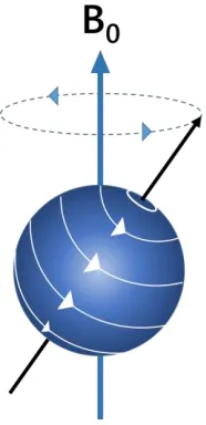
Nuclear magnetic resonance (NMR) spectroscopy can be used to exploit the intrinsic property possessed by certain atomic nuclei of “spin” Figure 1.4 and the fact that those nuclei that poses spin can undergo transitions between nuclear spin energy levels defined by the Zeeman quantised spin angular momentum, in order to determine the magnetic environment of the nuclei.

Figure 1.4 Single spin angular magnetic moment

An isolated nucleus has spin angular momentum and a precession frequency dependant only upon the type of nucleus (gyromagnetic ratio) and upon the strength of the applied magnetic field B0

Quantum mechanically sub atomic particles have intrinsic angular momentum, which is characterised by its spin quantum number I, where I is an integer or half integer. In a

number of atoms e.g. 12_C, 16_{O, spins are paired, cancelling each other out and result in an}

atom with no overall spin (I=0) and are therefore NMR-inactive. If the number of neutrons

and the number of protons in an atom are even then the nucleus has no spin, if the number of neutrons in addition to protons is odd then the nucleus will have half-integer spin (e.g. I=

P a g e| 18 spin (e.g. I= 1, 2, 3). The spin quantum number dictates magnitude of the angular magnetic

moment (μ) for the nucleus as related by Equation 1.

Where γ is the gyromagnetic ratio, this ratio is characteristic unique to each nuclear isotope. When an external magnetic field of strength B0 is applied, a spinning nucleus will align its

nuclear magnetic moment in a quantised number of orientations, given by 2I+1, either with

or against the magnetic field. For example in the case of a nucleus with spin I= ½, only one

transition is possible between two energy levels, the energetically favourable, aligned with the applied magnetic field (spin m= +½) also referred to as α and a higher energy orientation aligned against the applied magnetic field (spin m = -½) or β orientation (Figure 1.5), The splitting of these nuclear spin energy levels by the applied magnetic field is due to the Zeeman Effect, responsible for an identical splitting between each of the nuclear spin energy levels and is the dominant interaction in NMR. The distribution of these nuclear spin energy levels is governed by the Boltzmann distribution (Equation 2), where N values are the number of nuclei in each respective spin state, ΔE the energy level difference between each spin state (= ħω0) the strength of the external magnetic field, k the Boltzmann

constant and T the absolute temperature.

₍₂₎

P a g e| 19 large number of spectra to be collected in order to obtain adequate signal to noise. To improve sensitivity of NMR experiments, higher field strength magnets, that result in an increase in the size of the applied magnetic field, as well as decreasing the temperature at which experiments are conducted are two of the most common methods used in order to increase the Boltzmann distribution between the two energy states, thereby resulting in higher sensitivity.

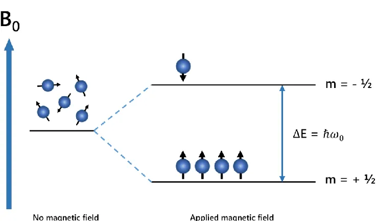
Figure 1.5 Zeeman splitting of energy levels

Illustration of Zeeman splitting of energy levels for a nucleus with spin I= ½. There are two possible Eigenstates for such nuclei, a low energy + ½ and a high energy – ½ state, The transition energy between the two states is related to the strength of the applied magnetic field and is described by the equation ΔE= ħω0. When a magnetic field is applied there is a Boltzmann

distribution of the spins in two states

1.4.2

Magnetisation

When a nucleus with angular momentum is placed in a magnetic field of strength B0 , the

P a g e| 20

Where ω is the angular velocity of precession, γ is the gyromagnetic ratio of the nuclide, Bo

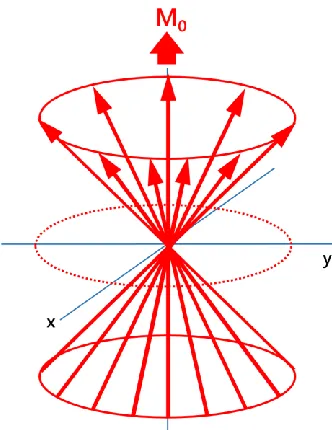
is the external, static magnetic field and the sign denotes the direction of motion of the magnetic moment about the static field. In a real sample there are a large number of nuclear spins in the system, all pressing about the z-axis (Figure 1.6), this ensemble of nuclei of the same kind, would precess around the applied magnetic field with a common angular frequency, giving rise to a net resultant bulk magnetisation, i.e. the sum of all individual magnetic moments, M0.

Figure 1.6 Orientation and precession of nuclear spins

An ensemble of nuclear magnetic moments (red arrows) distributed across the two spin energy levels, will precess around the magnetic field B0 without any phase coherence. The excess

P a g e| 21

1.4.3

R.F pulses and the Rotating Frame

Once a sample is placed the NMR spectrometer, the nuclear spins will align with the applied magnetic field B0 where they will reach equilibrium with a bulk magnetisation. Nuclear

magnetic resonance occurs when electromagnetic radiation with a frequency matching with the Larmor frequency of the nuclei of interest is applied in order to perturb the magnetic moments (as shown in Figure 1.7), causing the nuclei to change its spin state. Using the rotating frame coordinate system (x’, y’ and z), where the external magnetic field is considered to be along the z-axis, a radio frequency (RF) pulse of radiation is applied along the x’-axis (B1), this will impose a torque on the bulk magnetisation vector (M0) resulting

from the precessing nuclei (B1 and M0 are stationary and at right angles in the rotating

frame of reference).

Figure 1.7 Magnetisation and rotating frame of reference

(A) Bulk magnetisation M0 at thermal equilibrium precessing in the z-axis in the magnetic field

B0. (B) Application of a 90° (π/2) RF pulse in the B1 x’-axis causes perturbation of the bulk

magnetisation vector, rotating it into the y’-axis. (C) Once the RF pulse is switched off, the bulk magnetisation vector relaxes back gradually to thermal equilibrium, precessing around the y,z plane giving rise to the FID signal recorded in the detector.

This torque will be perpendicular to the external field vector and rotates the bulk magnetisation vector M0 away from its equilibrium position along B0 and around into the

P a g e| 22 plane (in which the detector is placed), causing a very weak oscillating voltage to be induced in the coil surrounding the sample, which is responsible for the observed NMR signal. The angle of rotation (θ), is dependent upon the gyromagnetic ratio of the nucleus γ, the amplitude of the B1 RF pulse and upon the length time (t) that the pulse is applied, (as

given in Equation 4), the example of a 90° or π/2 pulse is given in Figure 1.7 B. Once the applied RF pulse is switched off, the system undergoes relaxation, with the bulk magnetisation vector gradually returning back to its thermal equilibrium state along the z-axis, this is referred to as longitudinal (T1) relaxation. Whilst T1 relaxation describes the decay

of signal back into the z-axis, transverse (T2) relaxation characterises the relaxation in the

transverse (xy) plane as a result of excited nuclei exchanging spins or loosing coherence with each other and is therefore also referred to as ‘spin-spin’ relaxation. This relaxation back to thermal equilibrium causes the signal observed in the receiver coil to decay with time.

P a g e| 23

Figure 1.8 Free Induction Decay (FID)

A Free Induction Decay (FID) signal produced as a result of relaxation of excited spins in an NMR experiment, Fourier transformation of which gives rise to a frequency domain spectrum.

1.4.4

Chemical Shift

P a g e| 24 between the position of the signal of interest and that of the reference is termed the chemical shift.

NMR chemical shift values are typically expressed in ppm rather than in Hz, so as to remove the dependency of the magnetic field strength (operating frequency) at which the

sample was recorded using Equation 5.

Where is the Larmor frequency for a reference compound, e.g.

tetramethylsilane (TMS) for 1_{H or 4,4-dimethyl-4-silapentane-1-sulfonic acid (DSS) for} 13_C.

This results in a scale that is independent of the applied external magnetic field B0 used for

the experiment. As nuclei in a complex sample such as a protein will experience different chemical environments resulting in differing Larmor frequencies, the resultant dispersion one dimensional (1D) NMR spectrum obtained can be much more complicated to interpret in comparison to simple ingle molecule samples due to the crowding and over lapping of signals, therefore multidimensional (two or three dimensional 2D/3D) experiments are typically used in order to simplify assignment of the chemical shifts recorded.

1.4.5

Two dimensional (2D) NMR

A number of homo-nuclear 2D experiments exist, all of which share the same basic principle. There are four steps to a 2D NMR experiment; in the first step (called the preparation time), all nuclei in the sample are excited simultaneously using one or more pulses, creating magnetisation in the xy plane. The resulting magnetisation is allowed to evolve during the evolution period (t1) during which time encoding is carried out in the

P a g e| 25 followed by a mixing time (tmix) in which magnetisation is allowed to transfer to the second

nucleus (e.g. B) using either a combination of pulses or delay periods. The final stage is detection where the chemical shift of the second nucleus is recoded in the direct dimension

(F2). Raw data from a 2D NMR experiment consists of a series of FIDs, each one acquired

with a slightly longer t1 duration than the previous; the 2D data can then be Fourier

transformed in order to produce a 2D NMR spectrum. By selectively labelling specific residues of interest, the presence of cross-peaks off the diagonal in the 2D spectrum (Figure 1.9) obtained can provide information about which amino acids are close together in space. Such experiments make use of the structural information contained within through-space dipolar couplings by applying a recoupling sequence during the mixing time.

Figure 1.9 2D NMR experiment.

Representation of a 2D NMR spectrum shown on left, and a representation of peptide dimer with isotopic labels indicated as A, B and C. At short mixing times (green circle) magnetisation travels only far enough to see short range correlations (green cross peaks). At longer mixing times (red circle) the magnetisation is allowed to travel further and as such longer range correlations are observed (red cross peaks).

A

B

C

A

B

C

A

P a g e| 26

1.5

Solid state NMR

In solid state NMR (ssNMR) the samples being analysed are typically powder samples i.e. samples consisting of many crystallites in random orientations. The anisotropic nuclear spin interactions that affect ssNMR spectra such as; CSA, dipolar and quadrupolar coupling (as detailed in Section 1.3.4-6) are all dependent upon the orientation of crystallite orientations. In solution NMR this is not a problem as anisotropic interactions are averaged to zero, as molecules in solution exhibit Brownian motion, tumbling faster than the frequency of the interactions and reorientation of molecules occurs on the NMR timescale i.e. pico/nanoseconds (dependent upon the size of the molecule). By contrast, ssNMR experiments concentrate on solid samples with restricted molecular motion (i.e. milliseconds to seconds on the NMR timescale) where fast molecular tumbling does not exist, therefore the effect of anisotropic interactions, that are averaged out in solution NMR are still present in spectra obtained by ssNMR. Additionally, in solid samples molecules exist simultaneously in a number of orientations and as a result ssNMR spectra exhibit broad features, powder patterns composed of a superposition of signals from a number of different orientations. As a result ssNMR spectra contain significant structural information that is typically lost in solution NMR, although due to the lack of resolution in ssNMR spectra obscures any information that the spectrum may contain. Additionally due to the strong dipolar coupled network of spins, protons are generally not the preferred nuclei for observation in solid state NMR as these interactions typically result in broadened spectra. For ssNMR of protein samples structural details are primarily obtained from low-γ and dilute I=½ spins i.e. 13_{C and} 15_{N. The detection of low γ nuclei typically requires isotope}

enrichment for sensitivity enhancement. Therefore in order to obtain high resolution NMR spectra of solid samples, techniques such magic angle spinning (MAS) have been developed, whist methods such as cross-polarisation (CP) and high power proton decoupling, in order to remove 1_H-13_{C and} 1_H-15_{N couplings that are too strong to remove}

P a g e| 27

1.5.1

Magic angle spinning (MAS)

Magic angle spinning (MAS), first introduced by Andrew and Lowe (Andrew, Bradbury et al. 1959) is routinely used in solid state NMR to mimic the rapid isotopic tumbling that occurs in solution that does not occur in solid samples via mechanical rotation of the sample. MAS is essential for obtaining high resolution ssNMR spectra and is used to remove the effects of chemical shift anisotropy and to assist the removal of heteronuclear dipolar coupling. As shown in Figure 1.1 typically the sample filled rotor is spun about its axis at β = 54.74°, “the magic angle”, with respect to the magnetic field B0,

and is rotated at a rate . Spinning at the magic angle simulates the rapid isotropic tumbling that occurs in solutions, which averages the molecular orientation dependence of the transition frequencies to zero on the NMR timescale. Chemical shielding and dipolar

coupling both contain a molecular orientation dependence term of the form

with respect to the magnetic field B0. In solution the rapid tumbling averages this

component to zero thereby removing their effects, whereas in ssNMR this angular component can be averaged to zero by mechanically rotating and spinning at the magic angle.

B

₀

54.7°

Figure 1.10 Illustration of rotor assembly in a magic angle spinning experiment

The rotor containing sample is spun at 54.7° (magic angle) with respect to the magnetic field B0,