Can machine learning automatically choose your best model checking strategy?

Can machine learning automatically choose your best

model checking strategy?

Max Hendriks

The Netherlands

[email protected]

ABSTRACT

State space methods provide an automated way of verify-ing models. However, these methods suffer from the state space explosion problem. Many methods have been devel-oped to cope with this problem. As a result, a user has many different strategies to apply state space methods to models.

Because there is such a large amount of different strategies, it is hard for a user to select an appropriate strategy. If a bad strategy is selected, the model may be unsolvable, or waste resources. Additionally, the necessary intervention of a user makes the process of validation less automated. Therefore, it would be useful if the model checker itself is able to select an appropriate strategy. This would make the process fully automated and ensure that no resources are wasted.

To allow the model checker to predict a suitable strategy, it needs to use information present in the model itself. This research investigates to what extent the characteristics of Petri Net models can be used to predict an appropriate strategy. The performance of 532 different PNML models was determined using LTSMin for 20 selected strategies. This data was used to create a regressor for every strategy, which predicts the expected runtime when that strategy is applied to a given model. These regressors were then combined into a single classifier which could predict an appropriate strategy.

The classifier was compared to the best single strategy, and was shown to predict a strategy which outperforms this fixed strategy in %17 of the predictions, and results in an average time loss of 12.95 seconds.

Keywords

Machine learning, Model checking, Symbolic state space methods, Classification, Petri net features

1.

INTRODUCTION

Models are used to check the properties of different types of objects or processes, from computer programs, to the behaviour of electronic circuits, to protein synthesis. A popular way of analysing these models is using state space methods. These methods, however, suffer from the state space explosion problem, where a linear increase of model

Permission to make digital or hard copies of all or part of this work for personal or classroom use is granted without fee provided that copies are not made or distributed for profit or commercial advantage and that copies bear this notice and the full citation on the first page. To copy oth-erwise, or republish, to post on servers or to redistribute to lists, requires prior specific permission and/or a fee.

30thTwente Student Conference on ITFebr. 1st, 2019, Enschede, The Netherlands.

Copyright2018, University of Twente, Faculty of Electrical Engineer-ing, Mathematics and Computer Science.

size exponentially increases the amount of states the model can exist in [26]. This makes it really difficult to analyse large models. Many methods have been developed in the past decades to cope with this problem, and as a result, many different strategies exist to apply these methods on the analysis of models.

Since there are so many possible combinations of meth-ods that can be used, it can be extremely hard for a user, especially an inexperienced one, to select an appropriate strategy. A bad strategy may make the model unsolv-able or lead to an excessive waste of time and memory. If model checking tools were able to select the most suitable strategy by themselves without user intervention, it would ensure that resources are used optimally, and allow for a greater amount of automation.

These models contain features which might provide enough information to predict an appropriate strategy to analyse the model. This research aims to find these features and create a machine learning classifier capable of accurately predicting an appropriate strategy for model analysis.

If the classifier causes a larger number of models to be solved with fewer resources used, when compared to using a fixed strategy, the classifier can be considered a success.

If model checking tools themselves could decide what strat-egy to apply to verify a given model, more and larger models can be verified, with less trained personnel. This research will investigate whether machine learning algo-rithms can be used to select an appropriate strategy using only the information embedded within the model.

Is it possible to train a machine learning classifier, that recommends a strategy if given a model, which outperforms the use of a single strategy?

In order to recommend a strategy, the classifier needs in-formation (called features) of a model. This gives rise to the following research question:

What features can be found within models?

It is not necessary to train a classifier that finds the best strategy available. It is sufficient to train a classifier that finds a strategy, such that on average, it is better than using a fixed strategy.

2.

BACKGROUND

During the creation of software, it is almost impossible to create a fully fault-free product. An obvious way of in-creasing the quality of software is to track down and fix these faults. One popular way of achieving this is through testing, which can be a lengthy and costly procedure, and will not guarantee the absence of other errors. More ad-vanced techniques are necessary in order to guarantee the absence of errors, or guarantee the presence of other

Figure 1. Example of a Petri Net [7]

erties.

Formal verification is one such technique, allowing one to prove or disprove whether a program follows some speci-fied behaviour. When the presence of a desirable property cannot be proven, it may indicate that the program will not always behave according to specification. This infor-mation can then be used to improve the program.

Formal verification can also be used to verify properties of hardware, specifications of protocols or other designs. In the field of biology, formal verification can be used to analyse the behaviour of cells and other systems. It is common to create a specification which captures the most important behaviour of the object under verification. A model of the object is then checked on whether it meets that specification.

This research focuses Petri Net models. An example of a Petri Net can be seen in Figure 1.

2.1

State space methods

One form of formal verification is the verification of a model using state space methods. State space methods work by constructing the entire state space of a model, covering all possible states that it can exist in. The ques-tion for the object under verificaques-tion can then be answered by examining this state space. State space methods can be grouped into two distinct categories: Explicit meth-ods and Symbolic methmeth-ods. These categories differ in the way states are encoded during the exploration of a model. Explicit methods allocate a fixed amount of memory for each state, while symbolic methods use binary decision di-agrams (BDDs), or a variant of these, to store the state space.

A BDD is a graph, which like a tree, starts at a single root node and ends in one or more leaf nodes. Unlike a tree, nodes in a BDD may have more than one parent node and may interlink. A BDD is constructed in such a way, that every path through a BDD indicates a state of the model. This allows one to represent a large amount of states using relatively few nodes.

An example of a binary decision tree of a function f(x1,x2,x3) is shown in Figure 2. Its corresponding BDD is shown in Figure 3.

As mentioned above, the state space explosion problem makes it hard to analyse large models. To deal with this problem, a large number of measures have been developed. These measures include techniques such as partial order reduction, abstraction and the limiting to specific verifi-cation questions. Techniques to traverse the state space more efficiently have also been developed. Many different tools exist which implement one or more of these tech-niques [4]. As a result, end users have many options to

Figure 2. Binary decision tree [1]

Figure 3. Binary decision diagram corresponding to the Binary decision tree in Figure 2 [1]

consider when applying state space methods to their mod-els. Henceforth, we will call combinations of these tech-niques strategies. These strategies describe how a state space method is applied to a model, which in practice, could be the combination of the chosen algorithm with one or more settings of a tool. This research will make use of the tool called LTSMin [16].

One advantage of state space methods is that their process is mostly automated, but since there is such a large variety of strategies, users have to learn about the methods and tools before they can be used effectively. Furthermore, the large variety of models makes it almost impossible to learn a good strategy beforehand. Thus, finding a good strategy takes either a lot of experience, or a lot of trial and error. The strategies on which this research focuses on are discussed in Sections 3.2 and 3.3.

or may even cause the verification to fail. Ideally, the user only has to select the model for verification, and the verification tool itself will choose an appropriate strategy to verify the model without user intervention. This would allow for the optimal usage of the available resources.

3.

RELATED WORK

First, we will discuss several of the methods which aim to mitigate the state space explosion problem. Afterwards, we will examine previous work on strategy prediction.

3.1

BDD construction

The state space explosion problem manifests itself into the BDD node explosion problem for symbolic state space methods. It usually appears halfway during exploration, when the number of nodes in the BDD grows extremely fast before contracting into its final form, which is usually much more compact [13]. This peak size must be kept as small as possible so that larger models can be explored.

The size of a BDD depends on the way the variables are ordered within the BDD. Reordering these variables can reduce the size of the BDD, but determining the opti-mal order is an NP-complete problem [11]. This makes it unfeasible to perform reordering according to the best variable order during state space exploration.

Since maintaining the best variable ordering during ex-ploration is unfeasible, other methods were proposed to reduce the peak size of the BDD. Some methods aim to find a good order before exploration [14], [17], [24], others try to maintain a good ordering during exploration [23].

3.2

State space traversal methods

The way a BDD is constructed also depends on the order in which states are discovered during exploration. Because of this, the traversal algorithm used also affects the peak size of a BDD. Multiple traversal algorithms have been suggested over the past years.

The traditional breadth-first-search (BFS) algorithm is one algorithm suitable for state space exploration. An alter-native to this, is the algorithm called chaining, which was proposed by Roig et al in [22]. They applied chaining to Petri Nets and found that it resulted in an improvement in speed of two orders of magnitude when compared to BFS. These results were not verified on large models, however.

A variation of both BFS and chaining was proposed in [13], where all states are used instead of only the previous discovered layer of states. Their results show that these variations are slightly better than the original algorithms overall, but that they perform worse for some models. Ad-ditionally, they showed that chaining is marginally better than BFS, but this too was presented using only five se-lected models.

Sol´e et al [25] introduced four additional algorithms which were aimed at improving the state space exploration for concurrent systems, and found that in most cases an im-provement can be achieved. However, chaining was still found to be a good alternative to these algorithms.

3.3

Saturation

Saturation is a method which can drastucally reduce the peak size of a BDD [13] [12]. It works by firing only the transitions at a certain level of the BDD. Once all transi-tions at a level have been fired, it is saturated and a higher level is explored. By saturating all levels in the BDD, the size of the BDD can be kept small. This method has been reported to improve performance by several orders of

mag-nitude [12].

3.4

Strategy prediction

Pel´anek’s work is closely related to this research. He de-fined the properties of state spaces and specifies groups of state spaces [19],[21]. These characteristics were used to find an appropriate strategy for a model beforehand. This led to the development of EMMA, which implements the prediction strategy for a model [20]. However, his work is limited to explicit state space methods and only uses models from the BEEM database [18].

Heijblom’s work focused on symbolic state space methods [15]. He made use of the LTSmin toolset [16], which is a model checker that offers multiple state space exploration tools, multiple options to guide state space exploration and can be used for multiple types of models. In his re-search, Heijblom found that there is no single strategy that can solve all models optimally. He attempted to train a classifier that would try to optimise the compute-time of checking a model, and one that would try to optimise the memory-usage. Ultimately, the memory-optimising classi-fier was marginally better than using a fixed strategy, and the time-optimising classifier was decidedly worse than us-ing a fixed strategy.

In his research, he defined 11 features of models. These features are all derived from a matrix that is constructed from a model by LTSmin, which is called the ’dependency matrix’. This dependency matrix is an abstraction of a model, where the rows indicate nodes in the model and the columns indicate the transitions in the model. This ab-stract representation of a model does not include any lan-guage specific characteristics. The features are described in Table 1

4.

METHODOLOGY

In his study, Heijblom gathered a large amount of data, but the training of an effective classifier proved difficult. Since this lack of effectiveness is presumably caused by a lack of features, we first defined new features. To assist with this, we limited the pool of models to just Petri Nets. This allows us to use tools and features that are exclusive to Petri Nets.

4.1

Scope

The main goal of this research was to investigate whether using additional features of models could improve the pre-diction of an appropriate strategy. A strategy is defined as the way a state space method is applied to a model in order to calculate its state space. Any property of a model can be defined as a feature. In this section, it is ex-plained what strategies were examined and what features were considered in this research.

4.1.1

Selected strategies

In order to make testing feasible, the number of strategies that were considered had to be limited. In related work it can be seen that the traversal method and the satu-ration method can significantly influence the state space exploration of a model [15]. This is the reason that these elements were chosen to be variable and all other elements of a strategy were kept fixed.

Four different traversal methods were considered in this research. These were:bfs, bfs-prev, chain andchain-prev. bfsandchain are the standard BFS and chain algorithms as discussed in section 3.2, whilebfs-prev andchain-prev are the algorithms proposed by Ciardo [13], which only consider the states found at the previous level.

Feature Definition

State Vector Length Width of the dependency matrix.

Groups The number of transition groups. This corresponds to the number of rows in the dependency matrix. Bandwidth Maximum bandwidth of

all rows in the dependency matrix after variable re-ordering.

Profile Sum of the bandwidth of all rows in the dependency matrix after variable re-ordering.

Span Sum of the span of all

rows in the dependency matrix after variable re-ordering.

Average Wavefront Sum of the wavefront of all rows in the dependency matrix after variable re-ordering divided by the number of rows.

RMS Wavefront Root mean squared over the wavefront of all rows in the dependency matrix after variable reordering. Event Span (ES) Sum of the span of all

rows in the dependency matrix before variable re-ordering.

Normalised Event Span (NES)

Normalised version of Event Span which allows to compare dependency matrices of different sizes. Weighted Event Span

(WES)

Weighted variant ofEvent Span.

Normalised Weighted Event Span (NWES)

Normalised version of Weighted Event Span which allows to compare dependency matrices of different sizes

Table 1. Features Heijblom selected, based on metrics of the dependency matrix [15]

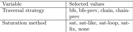
Variable Selected values

Traversal strategy bfs, bfs-prev, chain, chain-prev

Saturation method sat, like, loop, sat-fix, none

Table 2. Selected variables for the strategies.

Element Selected value

Regroup strategy tg,bs,hf save-sat-levels true

vset lddmc

lace-workers 1

sylvan-sizes 26,26,26,26

Table 3. Selected values of fixed aspects for all strategies

Four different saturation methods were included in this research. These were: sat, sat-like, sat-loop and sat-fix. In addition to selecting a saturation method, a saturation level must also be selected. From Heijblom’s research [15], it can be concluded that a saturation level of 5 gives a strategy the highest chance of successfully exploring the state space of a model. Therefore, the saturation level was chosen to be fixed at 5. The traversal methods were also considered without saturation, which has the value none. In this case, the saturation level is ignored.

In total, 20 different strategies were considered. The vari-ables and their selected values are given in Table 2.

Besides these variable elements of the strategies, there were also some fixed elements. These fixed elements are listed in Table 3. They were kept to be in-line with Hei-jblom’s research as much as possible [15]. The reorder strategy was chosen because it has the best performance overall [17]. save-sat-levels is a flag which enables some time optimisation for saturation. This flag has no effect when applied ifnoneis selected as the saturation method. vsetspecifies the package used for BDD construction. The other elements enforce that a fixed amount of resources is used when exploring the state space.

All other parameters of LTSMin that are not listed in ei-ther Table 2 or Table 3 keep their default values of LTSMin for version 3.0.2 for all strategies.

4.1.2

Selected features

All information contained within a model can be consid-ered as a feature. The features to be considconsid-ered had to be limited as well. Since the type of models was limited to models of the PNML filetype only, the features that could be considered was limited to those features that LTSMin is able to derive from any model, as well as any features specific to the PNML filetype.

In the Model Checking Contest [5], the models that are used have all had some of their properties checked and re-vealed beforehand. This is done using the CAESAR.BDD module from the CADP software package [2]. CAESAR.BDD is a software module which is used for the structural anal-ysis of Petri Nets. It can determine the values of many features in an automated fashion. These features are listed in Table 4. 4

Feature Definition

No. of places The number of places within a model

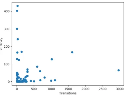
No. of transitions The number of transitions within a model

No. of arcs The number of arcs within a model

No. of unit The number of units within a model

Ordinary Boolean value whether all arcs within a model have a multiplicity of 1 Simple free choice Boolean value whether all

transitions sharing a com-mon input place have no other input place

Extended free choice Boolean value whether all transitions sharing a com-mon input place have the same input place

State machine Boolean value whether ev-ery transition has exactly one input place and ex-actly one output place Marked graph Boolean value whether

ev-ery place has exactly one input transition and ex-actly one output transi-tion

Connected Boolean value whether there is an undirected path between every two nodes (places or transi-tions)

Strongly connected Boolean value whether there is a directed path between every two nodes (places or transitions) Source place Boolean value whether

one or more places have no input transitions Sink place Boolean value whether

one or more places have no output transitions Source transition Boolean value whether

one or more transitions have no input places Sink transitions Boolean value whether

one or more transitions have no output places Loop-free Boolean value whether no

transition has an input place that is also an out-put place

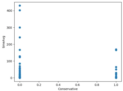
Conservative Boolean value whether for each transition, the num-ber of input arcs equals the number of output arcs Subconservative Boolean value whether for each transition, the num-ber of input arcs equals or exceeds the number of output arcs

Nested units Boolean value whether places are structured into hierarchically nested se-quential units

Safe Boolean value whether in

every reachable marking, there is no more than one token on a place

Deadlock Boolean value whether there exists a reachable marking from which no transition can be fired Reversible Boolean value whether

from every reachable marking, there is a tran-sition path going back to the initial marking Quasi-live Boolean value whether for

every transition t, there exists a reachable marking in which t can fire live Boolean value whether for

every transition t, from every reachable marking, one can reach a marking in which t can fire No. of reachable markings The number of

mark-ings reachable within the model

No. of transition firings The number of transition firings that can be trig-gered

Max. No. of tokens per place

The maximum number of tokens that can be at a single place

Min No. of tokens per marking

The minimun number of tokens that can exist within a marking

Max. No. of tokens per marking

The maximum number of tokens that can exist within a marking

Concurrent units The ratio of pairs of con-current units, the pairs of units Ui and Uj for which there exists at least one marking containing one place of Ui and one place of Uj.

Dead transitions The ratio of transitions which are not enabled in any reachable marking Exclusive places The ratio of pairs of places

Pi and Pj where there ex-ists no reachable marking containing both Pi and Pj

Table 4. Features extracted by the CAESAR.BDD module [5].

does not exist a subset of x for which a classifier trained with that subset performs equal or better than a classi-fier trained with x. Therefore, a minimal subset contains precisely the features necessary for the maximum perfor-mance of a classifier, while a non-minimal subset contains at least one redundant feature.

The minimal subset Profile, Span was chosen from Hei-jblom’s 11 features, since the values of these two features are determined with any standard run of LTSMin.

4.2

Techniques

This section discusses the models and techniques that were used during this research. First, the set of models that was used is discussed, then an overview of the tools and programs is given. Lastly, a list of the machines used for determining the performance of the selected strategies is provided.

4.2.1

Model Collection

The strategies selected above were tested on a large collec-tion of Petri Net models. The PNML models of the MCC were used [5]. Since LTSMin cannot handle colored Petri Nets, only the uncolored ones were used. This collection consists of 491 different models, which are instances of 66 parameterised Petri Nets. Furthermore, 42 models of the Petri Net Repository were considered [8]. In total, 532 models were considered.

4.2.2

Tools and programs

The following tools and programs were used during this research: Awk, Bash, Grep, LTSMin v3.0.2, Memtime, Python, R and Scikit-Learn.

4.2.3

Machines

The high performance computing cluster of the University of Twente was used to measure the performance of the selected strategies. Unfortunately, the 44 machines that Heijblom used, were not available on the SLURM cluster at the time of this research. Instead, 10 machines running Ubuntu 16.04.5 with 24GB of ram and two Intel XEON E5520 CPUs were used.

4.3

Method

This section describes the method which was used during this research in an attempt to answer the research ques-tions. The performance data of each selected strategy was determined for each selected model.

4.3.1

Data gathering

For every model, the exploration time of every strategy had to be determined. To do this, we made use of Hei-jblom’s scripts, which automatically generates jobs which can then be scheduled on the high performance cluster. To ensure that the performance measurements are accurate, every model was explored 10 times with every strategy, and the exploration time was averaged over these 10 runs. This means that in total, 532 (models) * 20 (strategies) * 10 (repetitions) = 106400 runs had to be completed.

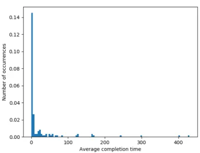
Because the amount of runs that needed to be completed was so great, a time limit of 30 minutes per run was set. This was intended to ensure that data gathering would not take too long. Since the regressors will attempt to predict the time it takes to complete an exploration for a given model, all runs that ran out of time had to be discarded. This is because it is impossible to guess how long it would take to complete a run without actually completing it. Additionally, any runs that failed due to an error, or that produced incorrect results were also discarded. This data

Figure 4. Histogram counting completion times for the bfs like strategy

refinement was done using a combination of Heijblom’s R scripts [15] and scripts newly created for this research. These new scripts as well as the collected data can be found in the author’s git repository [10]. In the end, only 127 models had runs that successfully completed in under 30 minutes for all strategies.

In addition to the low amount of datapoints that were actually usable, the completion time for these datapoints is also extremely skewed towards the low end. This can clearly be seen in Figure 4

In the most optimal situation, there would be an equal spread of datapoints across the whole possible time inter-val. Because the data is so skewed, the regressors will not be able to accurately predict the completion times of models that fall into the tail end of the histogram.

After refining the data, it was split up into seperate files, such that each file contains the performance data of each model for a specific strategy.

CAESAR.BDD was run on every model to collect the fea-tures it provides. To do this, the models first had to be converted from the PNML format into the NUPN format, which is used by the CADP software package. This is done using the PNML2NUPN tool, which can be downloaded from [9].

Once this process was finished, the performance data of every model for each strategy was combined with the fea-tureset collected by CAESAR.BDD. This resulted in 20 datasets, where every set contains the name of a model, the features collected for that model and the average ex-ploration time for a particular strategy.

4.3.2

Feature Relevance Analysis and Regressor

se-lection

First, a list of relevant features was created by plotting the features of each model against their average completion time for each strategy. These plots were examined for the presence of a potential correlation. Those features that showed no correlation with the completion time were discarded. The potentially relevant features that were left over are: Arcs, Conservative, Dead transitions, Deadlock, Places, Transitions, Profile, Span, Max tokens place and Min tokens marking. Plots of these features against the completion times of thebfs like strategy are presented in appendix A.

each strategy, all regressors in Scikit-Learn were tested. A python script was created which generates all possible subsets of the relevant features listed above. Then, for every strategy, every regressor in Scikit-Learn was trained using every possible subset of the relevant features. The training was done using a random selection of 66% of the data, and the regressors were tested using the remaining 33%. Since the training and testing data is selected ran-domly, this process was repeated 10 times. In order to compare the performance of every regressor and feature list combination, a metric in Scikit-Learn calledscorewas used, and its values were averaged over the 10 trials.

Thescoreis defined asscore= (1−u

v) whereu=

P

((ytrue−

ypred)2) and v= P((ytrue−ytrue)2). Here, ytrue is the

true value of the completion time, andypred is the value

predicted by the algorithm. ytrue represents the mean

value ofytrue. The maximum ofscoreis 1, which indicates

a regressor that predicts its values perfectly. A value of 0 indicates a regressor which always predicts the expected value, disregarding any input features. Note that the score of a regressor can be negative if it is worse than a regressor which always predicts the expected value.

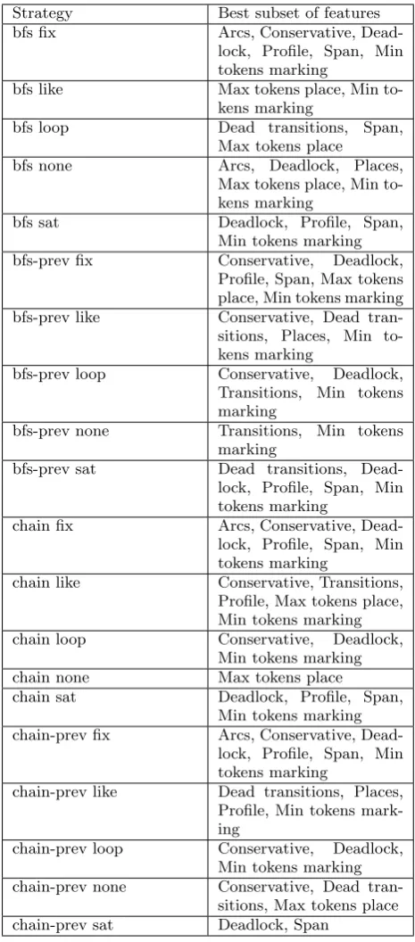
By comparing these scores, the best performing combi-nation of regressor and feature list was found for every strategy. The best subset of features for each strategy are listed in Table 5, and the best regressors and their average score for each strategy using the best subset of features are listed in Table 6.

4.4

Used regressors

This section will briefly describe the regressors that were used.

4.4.1

Ridge

Ridge is a linear regression algorithm which imposes a penalty on the size of its coefficients [3].

4.4.2

Elastic Net

The elastic net is a linear regression model, it is useful when there are multiple features that are correlated with one-another. It maintains the regularization properties of the Ridge algorithm, while also being able to learn a sparse model where few of the weights are non-zero, like Lasso [3].

4.4.3

Nearest neighbor regressor

The neighbors-based regression algorithm can be used in situations where the features are continuous rather than discrete values. It uses uniform weights where each point in the local neighbourhood contributes uniformly to the regression of a datapoint [6].

4.4.4

Decision trees

Decision trees are a machine learning method which use a collection of if-then-else rules to classify or regress. These rules are called splits, and divide the input data into boxes. Once this process has completed, the input data has been sorted into a leaf, which represents the outcome of the algorithm.

4.4.5

Random forest regressor

The random forest regressor is an enseble which is built up of a large amount of decision tree regressors. It is built from a sample drawn with replacement from the training set. Additionally, when splitting a node during the con-struction of a tree, the split that is chosen is not the best split, but rather it is the split that is the best among a random subset of the features. This randomness slightly

Strategy Best subset of features bfs fix Arcs, Conservative,

Dead-lock, Profile, Span, Min tokens marking

bfs like Max tokens place, Min to-kens marking

bfs loop Dead transitions, Span, Max tokens place

bfs none Arcs, Deadlock, Places, Max tokens place, Min to-kens marking

bfs sat Deadlock, Profile, Span, Min tokens marking bfs-prev fix Conservative, Deadlock,

Profile, Span, Max tokens place, Min tokens marking bfs-prev like Conservative, Dead tran-sitions, Places, Min to-kens marking

bfs-prev loop Conservative, Deadlock, Transitions, Min tokens marking

bfs-prev none Transitions, Min tokens marking

bfs-prev sat Dead transitions, Dead-lock, Profile, Span, Min tokens marking

chain fix Arcs, Conservative, Dead-lock, Profile, Span, Min tokens marking

chain like Conservative, Transitions, Profile, Max tokens place, Min tokens marking chain loop Conservative, Deadlock,

Min tokens marking chain none Max tokens place

chain sat Deadlock, Profile, Span, Min tokens marking chain-prev fix Arcs, Conservative,

Dead-lock, Profile, Span, Min tokens marking

chain-prev like Dead transitions, Places, Profile, Min tokens mark-ing

chain-prev loop Conservative, Deadlock, Min tokens marking chain-prev none Conservative, Dead

tran-sitions, Max tokens place chain-prev sat Deadlock, Span

Table 5. Strategies and their relevant features

Strategy Best regressor Score bfs fix Elastic net 0.50 bfs like Extra trees

re-gressor

0.24

bfs loop Extra trees re-gressor

0.09

bfs none Ridge 0.89

bfs sat Nearest neigbor regressor

0.46

bfs-prev fix Extra trees re-gressor

0.48

bfs-prev like Extra trees re-gressor

0.52

bfs-prev loop Extra trees re-gressor

0.41

bfs-prev none Extra trees re-gressor

0.95

bfs-prev sat Elastic net 0.49 chain fix Extra trees

re-gressor

0.48

chain like Extra trees re-gressor

0.36

chain loop Extra trees re-gressor

0.41

chain none Nearest neigh-bor regressor

0.03

chain sat Elastic net 0.44 chain-prev fix Extra trees

re-gressor

0.46

chain-prev like Extra trees re-gressor

0.21

chain-prev loop Extra trees re-gressor

0.22

chain-prev none Random forest regressor

0.09

chain-prev sat Elastic net 0.52

Table 6. Strategies, their best regressor and their score

Strategy Average completion time in seconds

bfs fix 20.21

bfs like 23.94

bfs loop 27.30

bfs none 84.64

bfs sat 7.92

bfs-prev fix 20.14

bfs-prev like 22.30 bfs-prev loop 30.38 bfs-prev none 79.74

bfs-prev sat 7.83

chain fix 20.12

chain like 18.62

chain loop 22.16

chain none 48.46

chain sat 7.93

chain-prev fix 20.10 chain-prev like 21.25 chain-prev loop 28.65 chain-prev none 41.64 chain-prev sat 7.98

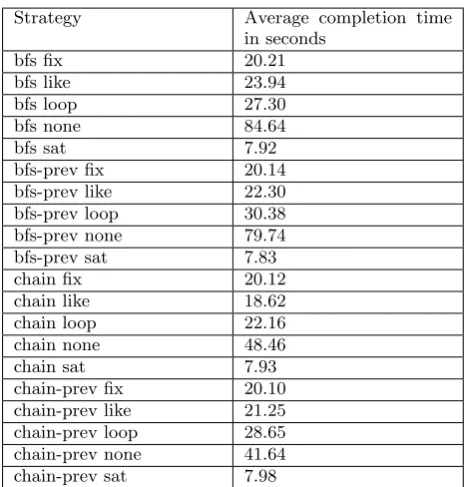
Table 7. Strategies and the average time they take to explore the models.

increases the bias of the forest, but it also decreases the variance.

4.4.6

Extra trees regressor

In the Extra trees regressor, the randomness in which the split is chosen is increased. Like in random forests, a ran-dom subset of candidate features is chosen, but instead of using the most discriminative thresholds, the thresh-olds are drawn at random for each feature, and the best of these randomly generated thresholds is chosen as the splitting rule. This allows for an even bigger reduction of variance when compared to the Random forest, but also results in a slightly higher bias.

4.5

Evaluation

As can be seen in Table 6, the maximum scores for the regressors of every strategy varies wildly. Some regressors, such as the one forbfs-prev none perform really well, but there are also regressors which score very poorly, such as the regressor ofbfs loop. There are two plausible reasons that these regressors perform so poorly. The first is that the feature list may simply not be adequate to predict the exploration time of a model. The second reason, which is more likely, is that there is simply not enough varied data.

The best combination of regressor and feature list for ev-ery strategy was combined into a single classifier. This classifier works by predicting the exploration time of a model for every strategy. The strategy for which its re-gressor predicts the lowest exploration time of a model, is selected as the strategy that should be used to explore that model. In order to evaluate this composite classifier, its predictions have to be validated.

To find out which strategy performs the best if it was the only strategy that could be used, the exploration times of all models were averaged for every strategy. The results of this process are shown in Table 7 The strategy for which the average exploration time is the lowest, isbfsprev sat. Therefore, this strategy was chosen to be the fixed strategy against which the composite classifier is compared.

which the exploration time is lowest, given a model. The exploration time of a strategy when given a model is com-pared against the exploration time of the fixed strategy for that same model. If the strategy predicted by the classi-fier has a lower or equal exploration time tobfs-prev none, it is considered to be a correct prediction. Otherwise, the prediction is counted as incorrect.

5.

RESULTS

The classifier attempted to predict a correct strategy for every model in its testing data. Since the training and testing data is selected at random, the evaluation is re-peated 100 times so that any variance is minimised. Since the testing data is 33% of the total amount of data, 0.33 * 127 ≈42 models were used to test the classifier every round.

The average amount of correct predictions is 7.01, versus the average amount of incorrect predictions of 34.99. This means that the Classifier predicts a suitable strategy 17% of the time. In addition to this, the difference in times be-tween the best fixed strategy and the predicted strategy is calculated and averaged over all trials. This indicates how close the strategies predicted by the classifier per-form when compared to the best fixed strategy. The test reported a loss in time of 12.95 seconds on average.

The scripts that were created, the programs that were used and the data that was collected can be found in the author’s git repository [10].

6.

CONCLUSION

The data collected from running experiments was used to extract data entries for 532 models, but the data from only 127 models was usable. 20 regressors, one for every selected strategy, were trained using Scikit-Learn. Every regressor was scored using Scikit-Learn’s score function, on data entries they were not trained with. These regressors were combined into a single classifier. This classifier was shown to recommend a strategy which is as good as or better than the best fixed strategy only %17 of the time.

This lack of performance clearly stems from the bad per-formance of every individual regressor. The classifier can only be as good as its worst regressor. Still, if the perfor-mance of the individual regressors can be improved, this technique of classification could work quite well.

7.

FUTURE WORK

The classifier performs really poorly in its current condi-tion. This mainly stems from the lack of accuracy of its component regressors. Future work would mainly consist of improving the performance of these regressors. Since some of the regressors, like the one for the bfsprev none strategy with a score of 0.95, perform quite well, the poor performance may stem from a lack of data rather than a lack of features. Therefore, the first step to improving this classifier would be to collect more data.

If the data collection were to be performed again, but with the 30 minute time limit removed, a lot more data would have been available. In addition, this data would be way more varied, since the longer exploration times of big mod-els would also be included. This would still probably leave a big gap in between the models with a low exploration time, and those that ran out of time, as the tail in Figure 4 decreased in size very rapidly. If the exploration times of big models is included, their exploration times would most likely fall outside of the scope of the histogram. So in addition to running the tests again without a time limit,

models need to be collected which have an exploration time located in this small tail. This would help round out the data, and minimise any gaps.

8.

ACKNOWLEDGEMENTS

First and foremost, I would like to thank my supervisors Doina Bucur and Jaco van de Pol for their valuable input and feedback during the project. Secondly, being able to use the scripts created by A. R. Heijblom saved a lot of time in this research. Finally, I would like to thank my friends and family for their support throughout my study and this research project.

9.

REFERENCES

[1] Binary decision diagram.https://en.wikipedia. org/wiki/Binary_decision_diagram. Accessed: 2019-01-27.

[2] Construction and analysis of distributed processes.

https://cadp.inria.fr. Accessed: 2018-12-02. [3] Generalized linear models.https://scikit-learn.

org/stable/modules/linear_model. Accessed: 2019-01-27.

[4] List of model checking tools.

https://en.wikipedia.org/wiki/List_of_model_ checking_tools. Accessed: 2018-11-29.

[5] Model checking contest.https://mcc.lip6.fr. Accessed: 2018-12-02.

[6] Nearest neighbors.https://scikit-learn.org/ stable/modules/neighbors.html. Accessed: 2019-01-27.

[7] Petri net.

https://en.wikipedia.org/wiki/Petri_net. Accessed: 2019-01-27.

[8] The petriweb collection.https://pnrepository. lip6.fr/pweb/models/all/browser.html. Accessed: 2019-01-19.

[9] Pnml to nupn converter. [10] Research git repository.

https://github.com/BurritoZz/ResearchProject. Accessed: 2019-01-27.

[11] B. Bollig and I. Wegener. Improving the variable ordering of obdds is np-complete. ieee trans. comput. 45(9), 993-1002.Computers, IEEE Transactions on, 45:993 – 1002, 10 1996. [12] G. Ciardo, G. L¨uttgen, and R. Siminiceanu.

Saturation: An efficient iteration strategy for symbolic state—space generation. In T. Margaria and W. Yi, editors,Tools and Algorithms for the Construction and Analysis of Systems, pages 328–342, Berlin, Heidelberg, 2001. Springer Berlin Heidelberg.

[13] G. Ciardo, R. Marmorstein, and R. Siminiceanu. The saturation algorithm for symbolic state-space exploration.International Journal on Software Tools for Technology Transfer, 8(1):4, Nov 2005.

[14] O. Grumberg, S. Livne, and S. Markovitch. Learning to order BDD variables in verification.CoRR, abs/1107.0020, 2011.

[15] A. Heijblom. Using features of models to improve state space exploration.

https://fmt.ewi.nl/education/master/207, December 2016.

[16] G. Kant, A. Laarman, J. Meijer, J. C. van de Pol, S. Blom, and T. van Dijk. Ltsmin:

High-performance language-independent model checking. In21st International Conference on Tools

and Algorithms for the Construction and Analysis of Systems, volume 9035, pages 692–707, April 2015. [17] J. Meijer and J. van de Pol. Bandwidth and

wavefront reduction for static variable ordering in symbolic reachability analysis. In S. Rayadurgam and O. Tkachuk, editors,NASA Formal Methods, Lecture Notes in Computer Science, pages 255–271. Springer International Publishing, 6 2016.

[18] R. Pel´anek. Beem: Benchmarks for explicit model checkers. In14th International SPIN Workshop: Model Checking Software, volume 4595, pages 263–267, July 2007.

[19] R. Pel´anek. Model classifications and automated verification. In12th International Workshop on Formal Methods for Industrial Critical Systems, volume 4916, pages 149–163, July 2007.

[20] R. Pel´anek and V. Roseck´y. Emma: Explicit model checking manager (tool presentation). In16th International SPIN Workshop on Model Checking of Software, volume 5578, pages 169–173, June 2009. [21] R. Pel´anek and P. ˇSimeˇcek. Estimating state space

parameters. InProceedings of the 7th International Workshop on Parallel and Distributed Methods in Verification, 2008.

[22] O. Roig, J. Cortadella, and E. Pastor. Verification of asynchronous circuits by bdd-based model checking of petri nets. In G. De Michelis and M. Diaz, editors,Application and Theory of Petri Nets 1995, pages 374–391, Berlin, Heidelberg, 1995. Springer Berlin Heidelberg.

[23] R. Rudell. Dynamic variable ordering for ordered binary decision diagrams. InProceedings of the 1993 IEEE/ACM International Conference on

Computer-aided Design, ICCAD ’93, pages 42–47, Los Alamitos, CA, USA, 1993. IEEE Computer Society Press.

[24] R. Siminiceanu and G. Ciardo. New metrics for static variable ordering in decision diagrams. pages 90–104, 03 2006.

[25] M. Sol´e and E. Pastor. Traversal techniques for concurrent systems. In M. D. Aagaard and J. W. O’Leary, editors,Formal Methods in

Computer-Aided Design, pages 220–237, Berlin, Heidelberg, 2002. Springer Berlin Heidelberg. [26] A. Valmari. The state explosion problem. In

W. Reisig and G. Rozenberg, editors,Lectures on Petri Nets I: Basic Models, pages 429–528. Springer-Verlag, June 2005.

10.

APPENDIX A

This appendix contains plots of all relevant features against the completion time for every data point of the bfs like strategy.

Figure 5. Value of Arcs of models against their average completion time

Figure 7. value of Dead transitions of models against their average completion time

Figure 8. Value of Deadlock of models against their average completion time

Figure 9. Value of Max tokens place of models against their average completion time

Figure 10. Value of Places of models against their average completion time

Figure 11. Value of Profile of models against their average completion time

Figure 12. Value of Span of models against their average completion time