University of Warwick institutional repository: http://go.warwick.ac.uk/wrap
A Thesis Submitted for the Degree of PhD at the University of Warwick
http://go.warwick.ac.uk/wrap/66339
This thesis is made available online and is protected by original copyright. Please scroll down to view the document itself.
Sequential Sample Size Re-estimation in Clinical
Trials with Multiple Co-primary Endpoints
by
Lupetu Ives Ntambwe
Thesis
Submitted in partial fulfilment of the requirements
for the degree of
Doctor of Philosophy in Health Sciences
Department of Medicine
Contents
List of Tables xiv
List of Figures xv
Acknowledgments xviii
Declarations xix
Abstract xx
Chapter 1 Introduction and Background 1
1.1 Introduction . . . 1
1.2 Concepts . . . 4
1.2.1 Notation and Definition of terms . . . 4
1.2.2 Clinical trials . . . 6
1.2.2.1 Definition and Phases of a clinical trial . . . 6
1.2.2.2 Clinical trials context . . . 7
1.2.3 Normal distribution . . . 8
1.2.4 Nuisance parameter . . . 11
1.2.5 One-sided test . . . 12
CONTENTS iii
1.2.6 Fixed Sample Z-test . . . 13
1.2.7 Fixed sample t-test . . . 15
1.2.8 Significant tests and P-value . . . 16
1.2.9 Motivation of sequential analysis . . . 18
1.3 Multiple endpoints . . . 21
1.3.1 Introduction . . . 21
1.3.2 Family-wise type I error rate ( FWER ) . . . 22
1.3.2.1 Definition of family of hypotheses . . . 22
1.3.2.2 Preliminaries . . . 22
1.3.2.3 Individual and familywise error rate . . . 23
1.3.2.4 Control of FWER . . . 24
1.3.3 Methods for controlling FWER . . . 25
1.3.3.1 Single-step procedures . . . 25
1.3.3.1.1 Bonferroni procedure . . . 25
1.3.3.1.2 Sid˘ `akprocedure . . . 27
1.3.3.2 Stepwise procedures . . . 27
1.3.3.2.1 Holm procedure . . . 28
1.3.3.2.2 Hochberg procedure . . . 28
1.3.3.2.3 Hommel procedure . . . 29
1.3.4 Disjunctive Power . . . 30
1.4 Multiple co-primary endpoints: General framework of analysis . . . 31
1.4.1 General framework of analysis for the sample size re-estimation approach . . . 31
iv CONTENTS
1.5 Summary . . . 34
Chapter 2 Literature review 35 2.1 Sample Size Re-estimation (SSR) with a single endpoint . . . 35
2.1.1 Introduction . . . 36
2.1.2 A framework for the analysis of a SSR . . . 37
2.1.3 Formulation of the problem . . . 38
2.1.4 Unblinded methods . . . 38
2.1.4.1 Stein’s Method . . . 39
2.1.4.2 Wittes and Brittain Method (the naive t-test) . . . 40
2.1.4.3 Birkett and Day procedure . . . 42
2.1.4.4 Denne and Jennison procedure . . . 42
2.1.4.5 Wittes et al. and Coffey and Muller procedure . . . 43
2.1.4.6 Kieser and Friede procedure . . . 43
2.1.4.7 Miller procedure . . . 43
2.1.5 Blinded methods . . . 44
2.1.5.1 Gould and Shih procedure . . . 44
2.1.5.2 Zucker et al. procedure . . . 46
2.1.5.3 Gould and Shih procedure . . . 46
2.1.6 SSR: Methodology for a single endpoint . . . 46
2.1.6.1 Hypotheses, test procedures and sample size calculation . 47 2.1.6.2 Sample size re-estimation and test procedures . . . 48
2.1.6.2.1 Sample size re-estimation . . . 48
2.1.6.2.2 Type I error rate . . . 48
CONTENTS v
2.2 SSR Inverse Normal Combination test method with a single endpoint . . . . 50
2.2.1 Introduction . . . 50
2.2.2 Two-stage combination test . . . 50
2.2.3 Two stage Inverse Normal method . . . 52
2.2.3.1 Framework of analysis . . . 53
2.2.3.1.1 Step 1 . . . 53
2.2.3.1.2 Step 2 . . . 53
2.2.3.1.3 Step 3 . . . 54
2.2.3.2 Characteristics of the Inverse normal combination test . . 55
2.2.4 SSR Inverse Normal Combination test method: Methodology for a single endpoint . . . 56
2.2.4.1 Hypotheses and Test procedures . . . 57
2.2.4.2 SSR Inverse Normal Combination test: Motivation . . . . 58
2.3 Group Sequential Designs with a single endpoint . . . 60
2.3.1 Introduction . . . 60
2.3.2 Elements of a sequential method . . . 61
2.3.2.1 Parametrisation of treatment difference . . . 62
2.3.2.2 Test statistics and distribution theory . . . 63
2.3.2.2.1 Single normal sample with known variance . . 64
2.3.2.2.2 A more general distribution . . . 67
2.3.2.3 Stopping rules . . . 68
2.3.2.3.1 Pocock’s Test . . . 70
2.3.2.3.2 O’Brien and Fleming’s Test . . . 70
2.3.2.3.3 Spending function approach . . . 71
vi CONTENTS
2.3.4 Post-trial analysis . . . 75
2.4 Group Sequential Inverse Normal combination tests with a single endpoint . 76 2.4.1 Introduction . . . 76
2.4.2 Representing GSD tests as a Combination rule of j independent p-values . . . 78
2.4.3 Stopping rules . . . 79
2.4.4 GSD Inverse Normal combination test: Motivation . . . 80
2.5 Summary . . . 82
Chapter 3 Methods for sample size re-estimation with multiple co-primary end-points without early stopping 83 3.1 Sample Size Re-estimation with Multiple Co-primary Endpoints . . . 83
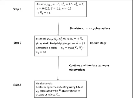
3.1.1 Framework for the analysis of a SSR with multiple co-primary endpoints . . . 84
3.1.2 Formulation of the problem . . . 86
3.1.3 Test statistics . . . 86
3.1.3.1 Implications for the FWER . . . 88
3.1.3.2 Implications for the power . . . 88
3.1.4 Sample size calculation . . . 89
3.1.5 Implementation of the method . . . 90
3.1.5.1 Step 1 - Initial sample size calculation . . . 91
3.1.5.2 Step 2 - Sample size re-estimation . . . 91
3.1.5.3 Step 3 - Final analysis . . . 92
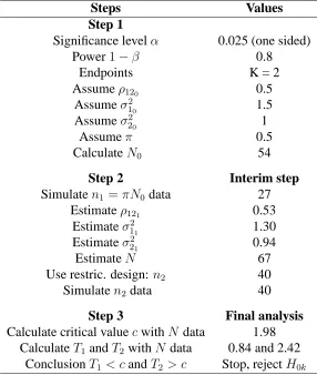
3.1.6 Example: SSR with Multiple Co-primary Endpoints . . . 92
CONTENTS vii
3.1.7.1 Power in the fixed sample size design for the guess
val-ues of the nuisance parameters . . . 97
3.1.7.2 FWER, power and sample size in SSR design . . . 99
3.1.7.2.1 Scenario 2 : FWER in Settings 1 - 5 . . . 99
3.1.7.2.2 Scenario 2 : Sample size in Settings 1 - 5 . . . . 100
3.1.7.2.3 Scenario 2 : Power in Settings 1 - 5 . . . 100
3.1.7.2.4 Scenario 3: Constantρ12 . . . 103
3.1.7.2.5 Scenarios 2 and 3: Summary and comments on the results . . . 103
3.1.7.3 Different effect sizes . . . 106
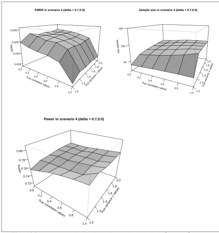
3.1.7.3.1 Scenario 4:δ1 = 0.5, δ2 = 0.7 . . . 106
3.1.7.3.2 Scenario 4:δ1 = 0.7, δ2 = 0.5 . . . 106
3.1.7.3.3 Scenario 4: Summary and comments on the re-sults . . . 109
3.1.7.4 SSR: Different timings . . . 109
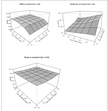
3.1.7.4.1 Scenario 5:π = 0.10 . . . 109
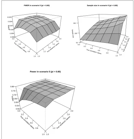
3.1.7.4.2 Scenario 5:π = 0.8 . . . 111
3.1.7.4.3 Scenario 5: Summary and comments on the re-sults . . . 111
3.2 SSR Inverse Normal Combination test for multiple co-primary endpoints . . 114
3.2.1 Framework for the analysis of the method . . . 114
3.2.1.1 Step 1 - Initial sample size calculation . . . 114
3.2.1.2 Step 2 - Sample size re-estimation . . . 114
3.2.1.3 Step 3 - Final analysis . . . 115
viii CONTENTS
3.2.3 Test statistics . . . 116
3.2.3.1 Implication for the FWER . . . 117
3.2.4 Implementation of the method . . . 118
3.2.4.1 Step 1 - Initial sample size calculation . . . 118
3.2.4.2 Step 2 - Sample size re-estimation . . . 118
3.2.4.3 Step 3 - Final analysis . . . 119
3.2.5 Worked example of the method . . . 120
3.2.6 Simulation results . . . 121
3.2.6.1 FWER, power and sample size in the SSR inverse nor-mal combination test design . . . 122
3.2.6.1.1 Scenario 2 : FWER in Settings 1 - 5 . . . 122
3.2.6.1.2 Scenario 2 : Sample size in Settings 1 - 5 . . . . 122
3.2.6.1.3 Scenario 2 : Power in Settings 1 - 5 . . . 125
3.2.6.1.4 Scenario 3: Constantρ12 . . . 125
3.2.6.1.5 Scenarios 2 and 3: Summary and comments on the results . . . 125
3.2.6.2 Scenario 4: Difference effect sizes . . . 128
3.2.6.2.1 Scenario 4:δ1 = 0.5, δ2 = 0.7 . . . 128
3.2.6.2.2 Scenario 4:δ1 = 0.7, δ2 = 0.5 . . . 128
3.2.6.2.3 Scenario 4: Summary and comments on the re-sults . . . 131
3.2.6.3 Scenario 5: Different timings . . . 131
3.2.6.3.1 Scenario 5:π = 0.10 . . . 131
CONTENTS ix
3.2.6.3.3 Scenario 5: Summary and comments on the
re-sults . . . 134
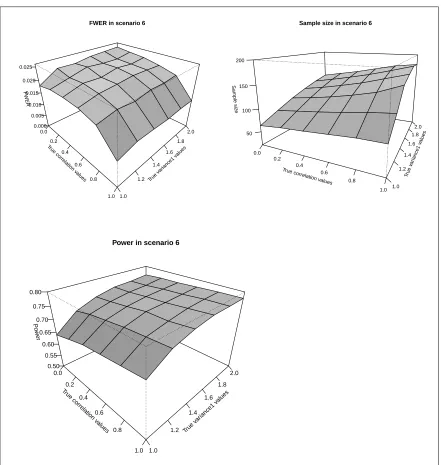
3.2.6.4 Scenario 6: Different weights . . . 134
3.2.6.4.1 Scenario 6: Summary and comments on the re-sults . . . 136
3.3 Summary findings from the simulation results . . . 136
Chapter 4 Group Sequential Designs with Multiple Co-primary Endpoints 140 4.1 Introduction . . . 141
4.1.1 Global methods . . . 141
4.1.2 Multiple hypothesis methods . . . 142
4.2 Group Sequential Designs with multiple co-primary endpoints . . . 144
4.2.1 Definition of the problems . . . 145
4.2.2 Test statistics . . . 145
4.2.3 Stopping boundaries . . . 149
4.3 Implementation of the method . . . 151
4.3.1 Before stage 1 . . . 151
4.3.2 Stage 1 . . . 152
4.3.3 Stage 2 . . . 153
4.3.4 Stage J . . . 155
4.3.5 Stage J + 1 . . . 156
4.4 Summary . . . 157
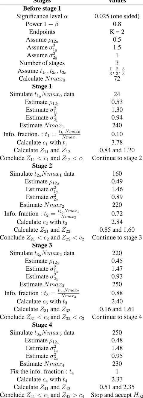
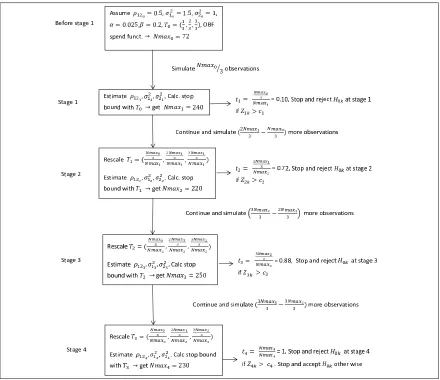
4.5 Example: Three-stage group sequential designs . . . 157
x CONTENTS
4.6.1 FWER, power and sample size in GSD with multiple co-primary endpoints . . . 164 4.6.1.1 Scenario 1 : Settings 1 - 5 . . . 166 4.6.1.1.1 Scenario 1 : FWER in Settings 1 - 5 . . . 166 4.6.1.1.2 Scenario 1 : Sample size in Settings 1 - 5 . . . . 166 4.6.1.1.3 Scenario 1 : Power in Settings 1 - 5 . . . 166 4.6.1.2 Scenario 2: Constantρ12. . . 169
4.6.1.3 Scenarios 1 and 2: Summary and comments on the results 169 4.6.2 Scenario 3: Different effect sizes . . . 172 4.6.2.1 Scenario 3: δ1 = 0.5, δ2 = 0.7. . . 172
4.6.2.2 Scenario 3: δ1 = 0.7, δ2 = 0.5. . . 172
4.6.2.3 Scenario 3: Summary and comments on the results . . . . 175 4.6.3 Scenario 4: Different spending function . . . 175
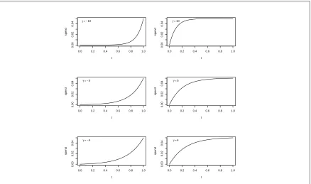
4.6.3.1 Scenario 4: Hwang-Shih-DeCani spending function with γ =−10 . . . 175 4.6.3.2 Scenario 4: Hwang-Shih-DeCani spending function with
γ = 10 . . . 178 4.6.3.3 Scenario 4: Summary and comments on the results . . . . 178 4.7 Summary findings from the simulation results . . . 179
Chapter 5 Group Sequential Design Inverse Normal Combination tests with
mul-tiple co-primary endpoints 181
CONTENTS xi
5.3 Group Sequential Inverse Normal Combination test Designs: Methodology
for multiple co-primary endpoints . . . 184
5.3.1 Definition of the problem . . . 184
5.3.2 Test statistics . . . 185
5.3.3 Stopping boundaries . . . 187
5.4 Implementation of the method . . . 189
5.4.1 Design stage . . . 189
5.4.2 Stage 1 . . . 190
5.4.3 Stage 2 . . . 191
5.4.4 Stage J . . . 193
5.4.5 Stage J + 1 . . . 195
5.5 Example: Three-stage GSD inverse normal combination test procedure for multiple co-primary endpoints . . . 199
5.6 Simulation results . . . 203
5.6.1 FWER, power and sample size in GSD Inverse Normal Combina-tion tests with multiple co-primary endpoints . . . 204
5.6.1.1 Scenario 1 : Settings 1 - 5 . . . 204
5.6.1.1.1 Scenario 1 : FWER in Settings 1 - 5 . . . 204
5.6.1.1.2 Scenario 1 : Sample size in Setting 1 - 5 . . . . 206
5.6.1.1.3 Scenario 1 : Power in Settings 1 - 5 . . . 206
5.6.1.2 Scenario 2 : Constantρ12 . . . 206
5.6.1.3 Scenario 1 and 2: Summary and comments of the results . 211 5.6.2 Scenario 3 : Different size effect . . . 211
5.6.2.1 Scenario 3 :δ1 = 0.5, δ2 = 0.7 . . . 211
xii CONTENTS
5.6.2.3 Scenario 3: Summary and comments on the results . . . . 213
5.6.3 Scenario 4: Different spending function . . . 213
5.6.3.1 Scenario 4: Hwang-Shih-DeCani spending function with γ =−10 . . . 213
5.6.3.2 Scenario 4: Hwang-Shih-DeCani spending function with gamma = 10 . . . 216
5.6.3.3 Scenario 4: Summary and comments on the results . . . . 216
5.7 Summary findings from the simulation results . . . 218
Chapter 6 Discussion and Conclusions 220 6.1 Discussion . . . 220
6.1.1 Sample size re-estimation method . . . 220
6.1.2 SSR Inverse Normal Combination test method . . . 221
6.1.3 Group Sequential Designs method . . . 222
6.1.4 GSD Inverse Normal Combination test method . . . 223
6.2 Extensions and future work . . . 223
6.3 Conclusions . . . 226
Appendix A: SSR simulation program 227
Appendix B: SSR inverse normal combination test simulation program 233
Appendix C: Program to compute the boundaries of a GSD 240
Appendix D: Program to complute mean vector, covariance matrix and
multivari-ate probability function 245
List of Tables
1.1 Number of errors when testing K hypotheses . . . 23
3.1 SSR: Implementation of the method . . . 93
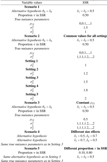
3.2 Initial values considered in the simulation study. . . 95
3.3 Scenarios considered in the simulation study. . . 96
3.4 Scenarios considered in the simulation study. . . 121
4.1 GSD: Implementation of the method . . . 158
4.2 Initial values considered in the simulation study. . . 163
4.3 Scenarios considered in the simulation study. . . 165
5.1 GSD: Implementation of the method . . . 198
5.2 Initial values considered in the simulation study. . . 204
List of Figures
1.1 Example of a p-value computation - licensed under the Creative Commons
Attribution-ShareAlike 3.0 . . . 18
2.1 Hwang-Shih-DeCani family of type I probability spending functions for various values ofγ . . . 74
3.1 SSR with multiple co-primary endpoints: Implementation of the method . . 85
3.2 Power in the fixed sample size design for two correlated endpoints . . . 98
3.3 SSR FWER in Scenario 2; Settings 1 - 5 . . . 101
3.4 SSR Sample size in Scenario 2; Settings 1 - 5 . . . 102
3.5 SSR Power in Scenario 2; Settings 1 - 5 . . . 104
3.6 SSR FWER, Sample size and Power in Scenario 3 . . . 105
3.7 SSR FWER, Sample size and Power in Scenario 4 (δ1 = 0.5,δ2 = 0.7) . . . 107
3.8 SSR FWER, Sample size and Power in Scenario 4 (δ1 = 0.7,δ2 = 0.5) . . . 108
3.9 SSR FWER, Sample size and Power in Scenario 5 (π= 0.10) . . . 110
3.10 SSR FWER, Sample size and Power in Scenario 5 (π= 0.8) . . . 112
3.11 SSR Combination test FWER in Scenario 2; Settings 1 - 5 . . . 123
3.12 SSR Combination test Sample size in Scenario 2; Settings 1 - 5 . . . 124
xvi LIST OF FIGURES
3.14 SSR Combination test FWER, Sample size and Power in Scenario 3 . . . . 127
3.15 SSR Combination test FWER, Sample size and Power in Scenario 4 (δ1 = 0.5,δ2 = 0.7) . . . 129
3.16 SSR Combination test FWER, Sample size and Power in Scenario 4 (δ1 = 0.7,δ2 = 0.5) . . . 130
3.17 SSR Combination test FWER, Sample size and Power in Scenario 5 (π= 0.1)132 3.18 SSR Combination test FWER, Sample size and Power in Scenario 5 (π= 0.8)133 3.19 SSR Combination test FWER, Sample size and Power in Scenario 6 . . . . 135
4.1 Group Sequential Designs with multiple co-primary endpoints: Implemen-tation of the method . . . 162
4.2 GSD FWER in Scenario 1; Settings 1 - 5 . . . 167
4.3 GSD Sample size in Scenario 1; Settings 1 - 5 . . . 168
4.4 GSD Power in Scenario 1; Settings 1 - 5 . . . 170
4.5 GSD FWER, Sample size and Power in Scenario 2 . . . 171
4.6 GSD FWER, Sample size and Power in Scenario 3 (δ1 = 0.5,δ2 = 0.7) . . 173
4.7 FWER, Sample size and Power in Scenario 3 (δ1 = 0.7,δ2 = 0.5) . . . 174
4.8 GSD FWER, Sample size and Power in Scenario 4 (γ =−10) . . . 176
4.9 GSD FWER, Sample size and Power in Scenario 4 (γ = 10) . . . 177
5.1 GSD Inverse Normal Designs with multiple co-primary endpoints: Imple-mentation of the method . . . 203
5.2 GSD combination FWER in Scenario 1; Settings 1 - 5 . . . 207
5.3 GSD combination Sample size in Scenario 1; Settings 1 - 5 . . . 208
5.4 GSD combination Power in Scenario 1; Settings 1 - 5 . . . 209
LIST OF FIGURES xvii
5.6 GSD combination test FWER, Sample size and Power in Scenario 3 (δ1 =
0.5,δ2 = 0.7) . . . 212
5.7 GSD combination test FWER, Sample size and Power in Scenario 3 (δ1 =
0.7,δ2 = 0.5) . . . 214
5.8 GSD combination test FWER, Sample size and Power in Scenario 4 (γ =
Acknowledgments
I would like to thank everyone who has supported me through the completion of this thesis. Firstly, I would like to show gratitude to my supervisor, Prof. Nigel Stallard, for teaching me about an interesting subject and for giving me valuable support and guidance throughout my PhD studies. I have also received valuable support from the supervision of Dr. Nicholas Parsons, who has provided valuable feedback on the manuscript. I must also mention Prof. Tim Friede for supervision at the beginning of my PhD studies.
I am grateful to the Engineering and Physical Sciences Research Council (EPSRC) and Novartis for the financial support of this PhD project. I am particularly grateful to Novartis for allowing me to present my works in Basel, Switzerland, towards the end of the project.
I would also like to thank all the administrative staff of the Warwick Medical School for making sure I was comfortable.
Declarations
Abstract
In this thesis, we consider interim sample size adjustment in clinical trials with multiple co-primary continuous endpoints. We aim to answer two questions: First, how to adjust a sample size in clinical trial with multiple continuous co-primary endpoints using adaptive and group sequential design. Second, how to construct a test in order to control the family-wise type I error rate and maintain the power, even if the correlationρbetween endpoints is not known.
To answer the first question, we conduct K different interim tests, each for one endpoint and each at levelα/K (i.e. Bonferroni adjustment). To answer the second question, either we perform a sample size re-estimation in which the results of the interim analysis are used to estimate one or more nuisance parameters, and this information is used to determine the sample size for the rest of the trial or the inverse normal combination test type approach; or we conduct a group sequential test where we monitor the information, and the information is adjusted to allow the correlationρto be estimated at each stage or the inverse normal combination test type approach.
Chapter 1
Introduction and Background
1.1
Introduction
The following problem is the main focus of this thesis: Suppose we have a study with two treatment groups, E (experimental) and C (control), which are to be compared in a parallel group randomised phase III clinical trial, and the same study has also K co-primary end-points. We want to control the family-wise type I error rate, which is defined as the prob-ability of falsely rejecting at least one null hypothesis among K hypotheses. We also want to control the power, knowing that it will depend on some nuisance parameters. Somehow we want to use interim data to modify the sample size to fix the power.
To resolve this problem, we will consider statistical methods for dealing with interim data. They will be sample size re-estimation, the group sequential approach and the inverse normal combination test procedure. Before reviewing these methods in more detail in the context of a single endpoint in the next chapter, this chapter gives some background on the concepts used throughout this thesis. Section 1.2 describes some of these concepts, Section 1.3 presents the concept of multiple endpoints, Section 1.4 describes the general framework of the analysis and Section 1.5 presents a summary.
end-point. Section 2.1 provides a background on the sample size re-estimation procedure with a single endpoint. This method enables the use of interim analyses of data to estimate one or more nuisance parameters. Following each interim analysis, this estimate is used to deter-mine the sample size for the remainder of the trial. Section 2.2 describes the inverse normal combination test method in the context of a single endpoint. This procedure enables the combination of interim data and final data at the final analysis. As is described, this analy-sis method can be used along with the sample size re-estimation approach. In Section 2.3, the group sequential design method is described, again in the setting of analysis of a single endpoint. This method allows a series of interim analyses to be conducted. As described below an error spending function can be used to ensure type I error control. Finally, in Section 2.4, the group sequential design inverse normal combination test method with a single endpoint is presented. This approach integrates the inverse normal combination test method into classical group sequential testing approach.
Chapter 3 presents the idea of sample size reestimation in the context of multiple co-primary endpoints. Section 3.1 presents a sample size reestimation approach for this setting, Section 3.2 describes the inverse normal combination tests method with multiple co-primary endpoints with sample size re-estimation and Section 3.3 presents a summary of the findings.
Chapter 4 describes group sequential designs in the context of multiple endpoints. The method uses specified stopping rules and a spending function based on the information at each interim analysis. This information is adjusted to allow for the estimated correlation, ρ, between test statistics at each stage.
Chapter 4.
1.2
Concepts
This section gives background and introduces some concepts and statistical tools required in the rest of this thesis. Notation and key terms are defined in Subsection 1.2.1, background on clinical trials is given in Subsection 1.2.2, whilst Subsections 1.2.3 to 1.2.8 give details of the normal distribution, nuisance parameters, one-sided tests, fixed sample Z-tests, fixed sample t-tests and p-values respectively. Finally, motivation for sequential analysis is given in Subsection 1.2.9.
1.2.1
Notation and Definition of terms
The following notation is used throughout this thesis.
(i) K represents the total number of co-primary endpoints; there are K endpoints. These will generally be labelled as k = 1,2,...,K.
(ii) J denotes total maximum number of stages or looks. The interim stages will generally be indexed by j, j = 1,...,J.
(iii) E denotes the experimental randomised, independently, identically distributed group and C represents the control randomised, independently, identically distributed group.
(iv) nEj (nCj) denotes the total number of randomised patients in group E (C) up to and including thejth stage and n
EJ (nCJ) represents a maximum sample size specified in advance. To simplify the notation, we assume that each group has equal sample size nEj = nCj, and denote this by nj. We finally assume that each group has a maximum sample size ofnJ and we denote this by N.
variable of thekthendpoint for theithsubject in group C at stage j (k= 1, ..., K, i= 1, ..., nCj, j = 1, ..., J).
(vi) E(XijkE) = θkE denotes the mean response for subjects receiving the experiment treatment E, and E(XijkC) =θkC represents the mean response for subjects receiving the control intervention C.
(vii) θkrepresents the mean difference between the two groups on thekth endpoint.
(viii) H0k:θk = 0is the null hypothesis for endpoint k.
(ix) δk is chosen to be a clinically important difference (or effect size) of interest and the alternative hypothesis isH1k:θk =δk.
(x) σ2
Ek(σCk2 ) represents the variance for response variableXijkE(XijkC). For simplic-ity, a common variance for endpoint k is considered i.e.σ2
Ek=σ2Ck=σk2.
(xi) ρk1k2 =corr(Xijk1, Xijk2)denotes the correlation betweenXijk1 andXijk2.
(xii) Σdenotes the variance covariance matrix between endpoints.
1.2.2
Clinical trials
1.2.2.1 Definition and Phases of a clinical trial
Pocock (2004) defines a clinical trial as any form of planned experiment that involves patients and is designed to elucidate the most appropriate treatment of future patients with a given medical condition. In conducting a clinical trial, one uses results based on a limited sample of patients to make inferences about how a treatment should be conducted among the general population of patients who will require treatment in the future. The clinical evaluation of a new drug is usually divided into four phases. The characteristics of each phase can differ between therapeutic areas, but can roughly be outlined as follows:
- Phase I includes the first experiments in human beings (often healthy volunteers). Such trials are primarily concerned with drug safety, not efficacy, and the first objec-tive is to determine how much of a drug can be given without causing serious side-effects. Studies of drug metabolism and bioavailability are also considered within this phase. Finally, in Phase I, studies of multiple doses are performed to determine the appropriate dose schedules for use in Phase II.
- In Phase II, the experimental treatment is first studied in patients with a view to an initial assessment of efficacy. This phase is also often used for identifying a safe and effective dose level for further development.
- In Phase III, a full-scale evaluation of a treatment is undertaken. The first objective is to compare the new drug, which has been shown as reasonably effective, with a placebo control or the current standard treatment(s) for the same condition in a large trial involving a substantial number of patients.
of morbidity and mortality. It is sometimes used to describe promotion exercises with the objective of bringing the new drug to the attention of a large number of clinicians.
The adaptive and sequential methods used in Phase III clinical trials are the main focus of this thesis. The primary goal in a Phase III clinical trial is usually to confirm whether or not the experimental drug (E) is efficacious compared to control (C). In a single setting, assume that the true treatment effect isθE for the experimental drug andθC for the control, and that a positive value of θE or θC indicates that the treatment has been useful to the patient. The treatment effectθ=θE−θC can then be assessed in a statistical hypothesis test context, where the null hypothesisH0 : θ = 0, is tested against the alternative hypothesis
H1 :θ >0. It is a regulatory requirement to control the type I error rate, the probability of
falsely rejecting the null hypothesis, at some pre-specified levelα. One-sided tests ofα =
0.025 are usually required by regulators, which correspond toα= 0.05 for two-sided tests. Also, with regard to the power at a certain value of the treatment effectθ=δ, it is necessary to make sure that it is at least 1 -β. β is the type II error, i.e the probability of failing to
reject the false null hypothesis. Popular choices forβ areβ= 0.1 andβ = 0.2.
1.2.2.2 Clinical trials context
The thesis also deals sample size re-estimation conducted in the context of a blinded
randomised clinical trial. Day and Altman (2000) explain that in controlled trials the term
blinding, and in particular double blinding, usually refers to keeping study participants
and those collecting and analysing clinical data unaware of the assigned treatment, so that they should not be influenced by that knowledge. Julious (2004) argues that blinding is important as it removes any systematic bias there may be in treatment assessment and allocation during the conduct of the trial. This forms the basis for regulatory authorities when deciding whether to approve a new drug.
1.2.3
Normal distribution
This thesis deals with sequential sample size re-estimation in clinical trials (with and with-out early stopping) with multiple continuous endpoints that follow normal distributions. In probability theory, the normal (or Gaussian) distribution is a continuous probability distri-bution and plays a central role in statistics.
In the setting of a single random variableX, the probability density function of a normal distribution is defined by
f(x) = √ 1
2πσ2e
−(x−θ)2
2σ2 (1.1)
for∞< x < ∞. The probability density function is dependent on two parameters, meanθand standard deviationσ, where∞< θ <∞andσ >0.
The expected value is
E(X) = Z ∞
−∞
xf(x)dx=θ (1.2)
V ar(X) = Z ∞
−∞
(x−θ)2f(x)dx =σ2 (1.3) wheref(x)is defined in Eq. (1.1).
Conventionally, N(θ, σ2) is used to indicate that a random variable X follows a
normal distribution with meanθand varianceσ2.
The standard normal distribution is a special case of the normal distribution where θ= 0 andσ2 = 1. Its density function is usually given by
φ(x) = √1
2πe −x2
2 (1.4)
and its distribution function is given by
Φ(x) = Z x
−∞
φ(x) = √1 2πe
−µ2
2 dµ. (1.5)
The variance defined in Eq. (1.3) is called the population variance in the sense that the concept of population can be extended to continuous random variables with infinite populations. However, in many practical situations, the true variance of a population is not known in advance and must be estimated on a sample of the population. Suppose we have a series of n measurements of a random variable X written asxi, where i = 1, 2, ..., n. The estimate sample variance is defined by
s2 = 1 n−1
n X
i=1
(xi−x)2 (1.6)
wherexdenote the sample mean of X .
(Bland (2000)). The answer to this is to take the square root, which will then have the same units as the observations and the mean. The square root of the variance is called the
standard deviation, usually denoted by s. Thus
s= v u u t 1
n−1 n X
i=1
(xi −x)2. (1.7)
Again, in the setting of two random variables X and Y, the probability density function of a normal distribution is defined by
f(x, y) = 1 2πσxσy
p
1−ρ2exp(−
1
2Q(x, y)) (1.8) where the quadratic form
Q(x, y) = 1 1−ρ2[(
x−θ1
σx
)2+ (y−θ2 σy
)2−2ρ(x−θ1)(y−θ2) σxσy
]
gives the density function of a bivariate normal distribution. Note that the parame-tersσ2
x,σy2, andρmust satisfyσx2 >0,σy2 >0, and0< ρ <1.
The correlation, ρ is defined as a bivariate analysis that measures the relation be-tween two or more variables such that systematic changes in the value of one variable are accompanied by systematic changes in the other (Bobko (2001)). In statistics, the value of the correlation coefficient is +1 in the case of a perfect positive (increasing) linear rela-tionship (correlation), - 1 in the case of a perfect decreasing (negative) linear relarela-tionship (anticorrelation). As the correlation coefficient value goes towards 0, the relationship be-tween the two variables will be weaker (closer to uncorrelated).
used to estimate the population correlation ρ between X and Y. The sample correlation coefficient is written
ρxy =
Pn
i=1(xi−x)(yi−y)
(Pni=1(xi−x)2)(Pni=1(yi−y)2)
(1.9)
wherexandyare the sample means of X and Y.
This can also be written as
ρxy = Pn
i=1(xi−x)(yi−y) (n−1)sxsy
wheresx andsy are the sample standard deviations of X and Y as defined in Eq. (1.7).
The correlation coefficient defined in Eq. (1.9) is called Pearson correlation. It is widely used in statistics and is the one we consider in this thesis. It measure the degree of the relationship between linear related variables. Other types of correlations include Kendall rank correlation and Spearman correlation; however, they are not discussed here as they are non-parametric tests used to measure the strength of dependence between two variables for the first and the degree of association between two variables for the second (Bland (2000)).
1.2.4
Nuisance parameter
example, if we are interested in the mean θ, the variance σ2 defined in Eq. (1.6) and the
correlationρxy defined in Eq. (1.9) are nuisance parameters.
The varianceσ2 and the correlationρ
xy may cease to be a nuisance if they become the object of the study. In general, a nuisance parameter is any parameter that interferes on the analysis of another.
To treat nuisance parameter in this thesis, we are going to use interim analysis to estimate the values of the nuisance parameter considered before the study begins, and this value is used to determine the parameter of interest (e.g. the sample size) for the rest of the trial or at interim stage.
1.2.5
One-sided test
Throughout this thesis, tests are conducted for the difference in the mean response of two treatments θ when observations are normally distributed with common, known (or unknown) varianceσ2.
The null hypothesis H0 : θ = 0 expresses that both treatments are equal. The
alternative hypothesis H1 : θ > 0 corresponds to one treatment being greater than the
other.
Suppose we have a standardised test statistic Z, which is normally distributed under H0, and a fixed sample test rejectsH0ifZ > cfor a constant c. The type I error probability
is defined as the probability of wrongly rejecting the null hypothesis,
α=P r(Z > c|θ = 0). (1.10)
P ower =P r(Z > c|θ =δ) = 1−β (1.11)
whereδrepresents a treatment difference that needs to be detected with high prob-ability andβ represents the type II error probability atθ =δ.
1.2.6
Fixed Sample Z-test
We consider a fixed sample test for a single endpoint. Let XiE and XiC i = 1,2,...,n, be theithobservations of samples E and C. We assume thatX
iE(XiC) is normally distributed with meanθE (θC) and a common and known varianceσ2 i.e.,XiE ∼ N(θE, σ2) (XiC ∼ N(θC, σ2)), and that all observations are independent. We are interested in testing a null
hypothesis that the two means are equal against an alternative hypothesis that the difference in means is a positive constant:
H0 :θE −θC = 0 H1 :θE −θC >0
If n subjects are allocated to each treatment, the standardised statistic (see Jennison and Turnbull (2000a), p. 22) is given by :
Z = p 1
(2nσ2)(
n X
i=1
XiE − n X
i=1
XiC)
∼ N((θE−θC) p
{n/(2σ2)},1). (1.12)
The information forθE −θC is:
I = n
So, underH0whereθE =θC,Z ∼N(0,1), and to satisfy the type I error probability requirement, we need:
P r(Z > c|θ= 0) =α (1.14)
where
c= Φ−1(1−α) (1.15)
represents the quintile of a normal distribution andΦdenotes the standard normal cumulative distribution function. The one-sided test with type I error probabilityαrejects H0 ifZ > c.
To satisfy the power requirement, we also need :
P r(Z > c|θ=δ) = 1−β (1.16) where Z ∼ N(θ√I,1) and θ = δ. We denote µ∗ = θ√I and call it the
non-centrality parameter. The power defined in Eq. (1.16) is now expressed by:
1−β = P r{Z−µ∗ > c−µ∗|θ =δ} 1−β = P r{−Z+µ∗ ≤ −c+µ∗|θ =δ} 1−β = Φ(−c+µ∗)
Φ−1(1−β) = −c+µ∗
µ∗ = c+ Φ−1(1−β).
The sample size n that satisfying the power requirement can be derived by replacing µ∗ byθp n
n= 2(Φ−
1(1−α)−Φ−1(1−β))2σ2
θ2 . (1.17)
Although we have based our test on the standardised test statistic Z, this is not the only possibility. Another test statistic is called the score statistic. It is defined in this case as:
S =Z√I (1.18)
where Z denotes the standardised test statistic and I the information. UnderH0, the
score statistic is normally distributed with mean 0 and variance I
S ∼N(0, I). (1.19)
UnderH1, the score statistic is normally distributed with meanθI and variance I
S ∼N(θI, I). (1.20)
1.2.7
Fixed sample t-test
In this subsection we consider the same problem and the same hypotheses as in Subsection 1.2.6. We assume thatXiE(XiC) is normally distributed with meanθE (θC) and a common and unknown varianceσ2.
The common varianceσ2can be estimated as follows;
S2 = (n−1)s
2
E+ (n−1)s2C
2n−2 (1.21)
where
s2E(C) = 1 n−1
n X
i=1
andxE (xC) denote the sample mean ofXiE(XiC).
The t-test is then given by
T = X¯E −X¯C
Sp2/n . (1.23)
Under the hypothesis of no treatment difference, T follows a t-distribution with
2n-2 degrees of freedom. Hence we reject the null hypothesis when T > t1−α,2n−2; where
t1−α,2n−2 is define as quintile of a t-distribution.
Under the alternative hypothesis that there is a clinical difference δ > 0, T follows a t-distribution with 2n-2 degrees of freedom and non-centrality parameter µ∗ defined in the
previous subsection as follows:µ∗ = √ δ
2S2/n >0.
The corresponding power can be written as
1−β =P(t1−α,2n−2−µ∗) (1.24)
whereP is the cumulative distribution. Practically one could use Eq. (1.17) for the initial sample size calculation and then calculate the power for this sample size using Eq. (1.23), iterating the sample size up as necessary until the required power is reached.
1.2.8
Significant tests and P-value
In Subsection 1.2.5 and Subsection 1.2.6, we explained that to carry out the test of signif-icance, we supposed that in the population, there is no difference between the two treat-ments. The hypothesis of no difference in the population was called the null hypothesisH0.
We then explained that if this is not true, then the alternative hypothesisH1 must be true,
that there is a difference between the treatments in one direction (or the other).
(i) Set up the null hypothesis and its alternative.
(ii) Find the value of the test statistic.
(iii) Refer the test to a known distribution (in our case a normal distribution) which it would follow if the null hypothesis were true.
(iv) Find the probability of a value of the test statistic arising which is as or more extreme than the one observed, if the null hypothesis were true.
(v) Conclude that the data are consistent or inconsistent with the null hypothesis.
The probability of such an extreme value of the test statistic occurring if the null hypothesis were true is often called the p-value. It (p-value) is well illustrated in Figure (1.1) and is used as an alternative to rejection points to provide the smallest level of sig-nificance at which the null hypothesis would be rejected. Its one sided form is defined mathematically as
p= 1−Φ(Z) (1.25)
where Z represents the standardized test statistic defined in Eq. (1.12) andΦ(.)the cumulative standard normal distribution function defined in Eq. (1.5).
The p-value can also be computed using t-test defined in Eq. (1.23), that is
p= 1−P(T, df) (1.26)
where P(.) denotes cumulative distribution anddf degree of freedom defined as
Figure 1.1: Example of a p-value computation - licensed under the Creative Commons
Attribution-ShareAlike 3.0
One often rejects the null hypothesis when the p-value is less than the predetermined one sided significance level 0.025, indicating that the observed result would be highly un-likely under the null hypothesis (i.e., the observation is highly unun-likely to be the result of random chance).
The p-value should not be confused with the type I error rate defined in Eq. (1.10). Even thoughαis also called a significance level, these two significance levels have different meanings. Their parent approaches are incompatible, and the numbers p and α cannot meaningfully be compared. The p-value is not the probability that the null hypothesis is true. The null hypothesis is either true or it is not; it is not random and has no probability. It is simply a measure of how likely the data is to have occurred by chance, assuming the null hypothesis is true (Bland (2000)).
1.2.9
Motivation of sequential analysis
Ethical. There is an ethical need to monitor the safety of patients in all treatment
arms when conducting clinical trials. For example, this can be done through sequential monitoring. Less patients are exposed to an inferior treatment than for the corresponding fixed sample design when a sequential trial is stopped early for a positive effect. Patients in the trial do not have to be exposed to potential side-effects of the drugs under investigation if a group sequential trial is stopped early for futility. Likewise, the resources that would have been necessary to complete the trial can instead be used to study a different treatment in the same or another area of medical necessity.
Administrative. Some of the administrative reasons given by Jennison and Turnbull
(2000a) for conducting interim analysis include the need to ensure that the experiment is conducted and executed as planned, that the subjects or experimental units are from the correct population and satisfy eligibility criteria, and that the test procedures or treatments are as prescribed in the protocol. A further administrative reason for early examination of study results is to check on assumptions made when designing the trial. For example, in an experiment where the primary response variable is quantitative, the sample size is often set assuming this variable to be normally distributed with a certain fixed variance. An early interim analysis can reveal inaccurate assumptions in time for adjustments to be made to the design. For example, Dmitrienko et al. (2005) explained that early evidence of efficacy may generate a decision to increase manufacturing spending in order to support continuing development of the experimental drug. However, to better help describe the efficacy and safety profiles of the drug, the trial may still be continued.
Economic. Sequential statistical procedures can also lead to economic benefits. For
size when compared with standard fixed sample methods. The authors also added that in-terim analyses allow informed management choices to be made concerning the continuing allocation of limited research and development funds.
Ethics is the most important and persuasive reason for sequential clinical trials. This is why most major trials now have a data monitoring committee (DMC), whose primary responsibility is to protect the safety of patients. For example, the ICH guideline E9 Statis-tical Principles for Clinical Trials encourages the use of interim monitoring through group sequential methods (ICH, 1998).
Three types of data monitoring may be considered in a blinded randomisation trial (Stallard and Todd (2010)): first, administrative monitoring of clinical trial conduct and monitoring of safety data without monitoring of efficacy data; second, monitoring of ef-ficacy data with no unblinding of treatment allocation. Stallard and Todd (2010) give an example of the estimation of nuisance parameters. Third, monitoring of efficacy data with treatment allocation unblinded to allow the estimation of the difference in efficacy between the treatments being compared. This (the third) type of monitoring presents the most ethical and statistical challenge. Stallard and Todd (2010) explain that in the second and the third type of data monitoring, administrative and safety monitoring will most likely be conducted in addition. This thesis focuses on the second and the third types of data monitoring.
1.3
Multiple endpoints
This section provides background on multiple endpoints in a clinical trial. It introduces various methods used to adjust for multiplicity. Subsection 1.3.1 is an introduction; Sub-section 1.3.2 defines and discusses the Family-wise type I error rate; SubSub-section 1.3.3 de-scribes methods for controlling family-wise type I error rate and Subsection 1.3.4 defines disjunctive power.
1.3.1
Introduction
A number of factors can influence the analysis, interpretation and conclusions drawn from a clinical trial. Among them are the disease under study, the patient population, multiple endpoints, the study design and the conduct of the study. One of the key factors that make interpretation difficult, and sometimes impossible, is the presence of multiple endpoints. Running a clinical trial with multiple endpoints may be justified by the nature of the disease and the type of questions that a clinical trial aims to investigate. For example, in patients with coronary heart disease, we may be interested in both resting and exercise ejection fractions. In blood-pressure-lowering trials, we might be interested in diastolic and systolic blood pressure or mean arterial pressure and pulse pressure. In stroke treatment, there are a number of scales used to measure recovery and no one scale is believed to assess all dimensions. In lung diseases, we may be interested in several lung function tests, such asF EV1, FVC, PI (Pocock et al. (1987)). In behavioral studies, we may be interested in
Conventionally, in testing a single hypothesis, the probability of a type one error (i.e. the probability of rejecting the null hypothesis when it is true) is usually controlled at some chosen levelα. For the setting considered here, this concept needs to be extended to the multiple testing situation to take account of the number of hypotheses tested.
1.3.2
Family-wise type I error rate ( FWER )
1.3.2.1 Definition of family of hypotheses
Throughout this thesis, a family of hypotheses is defined as a set of hypotheses for which significance statements are considered and errors jointly controlled ( Shaffer (1995)). Hochberg and Tamhane (1987) describes a family as any collection of inferences for which it is mean-ingful to take into account some combined measure of error.
Suppose we are considering testing a family of hypotheses,H0kagainst a family of alternative hypothesesH1k, k = 1,..,K. Suppose we do this using a series of test statistics Tk, k = 1,...,K. Suppose we also define the event thatH0k is rejected in preference ofH1k to beSk. To adjust for multiplicity, we need to control probabilities of disjunctive events of the formD = SKk=1Sk (Senn and Bretz (2007)). Note that the event D corresponds to rejecting at least one null hypothesis.
In this thesis we suppose that we are running a study for one purpose and the results are considered under one family of hypotheses. But if a study is used for different purposes, the results have to be considered under several different family configurations.
1.3.2.2 Preliminaries
Table 1.1: Number of errors when testing K hypotheses Null Hypotheses Not RejectH0 RejectH0 Total
True null U V K0
True alternative T S K−K0
Total W R K
the number of false declared null hypotheses (number of false positives or Type I error) and T denotes the number of false declared alternative hypotheses (number of false negatives or Type II error). R is the total number of null hypotheses rejections and W denotes the total number of non-rejections. K0 is the number of true null hypotheses, an unknown
parameters whereas K -K0is the number of true alternative hypotheses. U, V, S, T are not
observable, whereas R and W are observable.
1.3.2.3 Individual and familywise error rate
In the context of a single hypothesis, type I error rate is the probability of rejecting the null hypothesis when it is true. It is usually controlled at some chosen levelα, whereαis chosen by considering the costs of rejecting a true hypothesis as compared with those of accepting a false hypothesis. It is usually set to a conventional value of 0.025 (one sided). In the context of a family of hypotheses, type I error rate is the probability of falsely rejecting at least one null hypothesis in the family or the probability of at least one error in the family. It (type I error rate) is called the family-wise error rate (FWER) in this setting and is defined mathematically as below:
F W ER=P r(V >0) (1.28)
meaning the probability of making at least one type I error in the family,
or equivalently,
F W ER= 1−P r(V = 0). (1.29)
In connection to the event D (defined in Subsection 1.3.2.1), we may consider Pr(D) as the disjunctive type I error rate or FWER, that is:
Disjunctive type I error rate=P r(reject at least one falseH0k|θk = 0). (1.30) So, by assumingF W ER ≤ α, the probability of making at least one type I error in the family is controlled at levelα.
1.3.2.4 Control of FWER
In this thesis, we are going to test a family of hypotheses and will claim that the treatment in group E works against the one in group C if anyH0kis rejected, which means the FWER or disjunctive type I error rate. That is why we need to control the FWER. Some tests control the FWER only when all null hypotheses in the family are true, others control this error rate for any combination of true and false hypotheses. Hochberg and Tamhane (2001) refer to these as weak control and strong control, respectively. These concepts are discussed below.
The weak type controls the type I error only when all null hypotheses in the family are true: H0 =∩k∈KH0k, K0= K, whereK0 is the number of true null hypothesis defined in Table
1.1.
whereas the strong type controls the type I error for any partial configuration S (defined in Table 1.1) of the null hypotheses,K0 ≤K.
For FWER :maxS⊆KP(V >0| ∩k∈SH0k),k= 1, . . . , K.
1.3.3
Methods for controlling FWER
In Subsection 1.3.2, the FWER has been defined and type of controls of the FWER have been described. In this section, we review two methods for controlling the FWER. This includes single-step and stepwise methods. In the single-step procedure, the rejection or non-rejection of a single hypothesis does not depend on the decision on any other hypoth-esis. Bonferroni andSˇid`ak methods are cited as examples. Whereas in the stepwise sce-nario, the rejection or non-rejection of a particular hypothesis may depend on the decision on other hypotheses. As examples, we have the Holm procedure and Hochberg method.
Although both methods are described below, only the Bonferroni method will be considered as a method for adjusting the FWER in this thesis.
1.3.3.1 Single-step procedures
Single-step procedures use the same boundary for the rejection of hypotheses. Two single-step methods are described below.
1.3.3.1.1 Bonferroni procedure
Let us consider a set of p-values, p1, ..., pK, to test hypotheses H1, ...., HK. The Bonferroni procedure states that if any p-value is less than α/K, H0 = {H01, .., H0K}is rejected, whereH0 is the intersection of allH0k. This means that each hypothesisH0k (k = 1,. . . ,K) will be individually rejected ifpk ≤ α/K, whereα here is the overall level of significance. The Bonferroni inequality,
P r{ K [
k=1
(pk ≤α/K)} ≤α (1.31) ensures that the probability of rejecting at least one hypothesis when all are true is no greater thanα(Simes (1988)).
If the K endpoints are independent,
P r(smallest p-value≤α/K) = P r(rejecting at least oneH0k)
= 1−P r(not rejecting anyH0k)
= 1−(1−α/K)K = <1−(1−(α/K)K) = α
If the K endpoints are dependent,
P r(rejecting at least oneH0k) ≤
K X
k=1
P r(reject oneH0k|θk= 0)
= Kα/K (1.32)
= α
direction, Bonferroni’s procedure may lack power because the rejection of the overall hy-pothesis is based on the smallest p-value of the K test statistics.
In practice, endpoints are usually correlated. Pocock et al. (1987) show that Bon-ferroni’s correction practically works well for moderately correlated normally distributed endpoints with known variance and identical correlationρfor all possible pairs within the two compared groups. The conservatism of Bonferroni’s method increases asρincreases, but Bonferroni’s correction still performs well as the number of correlated endpoints in-creases.
1.3.3.1.2 Sid˘ ak` procedure
Bonferroni’s inequality was modified by Sidak (1967). Instead of testing each hypothesis atαk =α/K,Sid˘ `aksuggested using a level of significanceαk = 1−(1−α)1/K. Similar to Bonferroni’s approach,Sidˇ `akindicated that, for K independent endpoints:
P r(smallest p-value≤1−(1−α)1/K) = 1− {1−[1−(1−α)1/K]}K = 1−((1−α)1/K)K
= α
1.3.3.2 Stepwise procedures
Single step procedures use the same boundary for the rejection of hypotheses. Nevertheless, if different boundaries are assigned to different tests, testing methods may have a higher ability to preserve the FWER and to identify true alternative hypotheses. The following briefly describes three of them.
p-values. Consider ordering the p-valuesp(1), . . . , P(K)and let the associated null
hypothe-ses beH0(1), . . . , H0(K).
1.3.3.2.1 Holm procedure
Holm (1979) proposed a method that applies in the same cases as the Bonferroni procedure but is uniformly more powerful. His step-down method proceeds as follows.
Step 1. Ifp(1) < α/K, rejectH0(k)and go to Step 2; otherwise stop.
Step 2. Ifp(2) < α/K−1, rejectH0(2) and go to Step 3; otherwise stop.
· · ·
Step K. Ifp(K)< α, rejectH0(K)and stop.
The benefit of using Holm’s procedure is that the tests are made more powerful (smaller adjusted p-values) while, in most cases, maintaining strong control of the FWER. The method is based on the Bonferroni inequality and is valid regardless of the joint distri-bution of the test statistics. However, the downside of the procedure is that the stochastic (or random) dependencies between test statistics are not taken into account.
1.3.3.2.2 Hochberg procedure
Hochberg (1988) suggested a step-up method described as follows.
Step 2. Ifp(K−1) < α/2, rejectH0(k), k = 1,. . . ,K - 1, and stop, otherwise go to Step
3.
· · ·
Step K. Ifp(1) < α/K, rejectH0(k), k = 1, and stop.
The procedure is valid under independent or positively dependent p-values. Under independence, Hochberg’s method is more powerful than Holm’s, it maintains strong con-trol of the FWER. However, the problems with this procedure are that the stochastic (or random) dependencies between test statistics are not taken into account and it is only valid for positively correlated test statistics.
1.3.3.2.3 Hommel procedure
Hommel (1983) suggested a method that combines both step-up and step-down pro-cedures. The method is somewhat more powerful than Hochberg’s but is more difficult to understand and carry out. The method is as follows: reject all hypotheses that have a
p-valueα/k∗ wherek∗ is defined as
k∗ =max(kǫ{1, . . . , K}:p
(K−k+k⋆) >
k⋆α
k fork⋆ = 1, . . . , k).
If no maximum exists, all hypotheses are rejected (the largest p-value is then smaller thanα). To illustrate this method, we consider the example given by Ekenstierna (2004) that shows that Hommel’s procedure rejects more than Hochberg’s:
Suppose that we have three hypotheses H01, H02, H03 and the corresponding
p-valuesp1 = 0.012, p2 = 0.015, p3 = 0.0363. Letα be 0.025. With Hommel’s procedure
we first calculatek∗:
Fork= 2 : p3 = 0.0363> α= 0.025, p2= 0.015> α/2 = 0.0125.
Fork = 3 :p3 = 0.0363 > α= 0.025, p2 = 0.015 <2α/3 = 0.0167, p1 = 0.012>
α/3 = 0.000835.
Thus in this examplek∗ = max{1,2} = 2 and all hypotheses with a p-value ≤
α/2 = 0.0125 are rejected. The hypothesis with p-value p1 = 0.012 is then rejected
by Hommel’s procedure. If Hochberg’s procedure would be used instead, no hypotheses would be rejected: p3 = 0.0363 is larger than α = 0.025, p2 = 0.015 is larger than
α/2 = 0.0125andp1 = 0.012is larger thanα/3 = 0.00835.
As for Holm’s and Hochberg’s procedures, Hommel’s method maintains strong con-trol of the FWER. It is valid under independent or positively dependent p-values.
1.3.4
Disjunctive Power
Suppose we are considering testing a family of hypotheses,H0k, against a family of alter-native hypotheses,H1k, k = 1,..,K. Suppose we do this using a series of test statisticsTk, k = 1,...,K. In connection to the event D (defined in Subsection 1.3.2.1), we may consider Pr(D) as disjunctive power, that is:
Disjunctive power=P r(reject at least one falseH0k|θk =δk). (1.33) This thesis focuses mostly on the disjunctive. However, sometimes we may be inter-ested in the probabilities of conjunctive events of the form ofC=Tkk=1Sk. In connection to the event C, we may consider Pr(C) as conjunctive power, that is:
1.4
Multiple co-primary endpoints: General framework
of analysis
In this thesis, we consider methodology for situations where there are multiple continuous co-primary correlated endpoints in a clinical trial. This means that we are interested in obtaining significance in one of the endpoints. We also consider two different methods of analysing interim data: First, the sample size re-estimation method, in which data are used at one or more interim analyses to estimate nuisance parameters with this information used to determine the sample size for the remainder of the trial. Second, the group sequential designs approach, that includes a series of interim analyses with the possibility of stopping the trial at each analysis. Such a trial must be designed in advance, so as to maintain the FWER. The group sequential design method considered in this thesis is the combination of the concepts of early stopping and sample-size recalculation.
Based on concepts described previously in this chapter, the general framework for each of the two methods are defined in the following setting: There are two treatments, experimental E and control C.
1.4.1
General framework of analysis for the sample size re-estimation
approach
(i) To reiterate, letXikEbe the random variable of thekthendpoint for theithsubject in group E (k = 1, . . . , K, i = 1, . . . , nE) and XikC be the random variable of thekth endpoint for theithsubject in group C (k= 1, . . . , K, i= 1, . . . , n
C).
(ii) We consider one-sided tests as described in Subsection 1.2.5.
K co-primary endpoints are equal against an alternative hypothesis that the difference in mean vectors is a vector of positive constants:
H0k: θk= 0
H1k: θk=δk, (δk >0)
whereθkis the k’th element ofθ (a K x 1 column vector of true means) and we are testing a family of k hypotheses.
(iv) SupposeTk represents test statistics for endpoint k and cthe corresponding critical value observed at the end of the trial.
(v) To reiterate, we assume thatXikE(XikC) has a multivariate normal distribution lead-ing to a multivariate normal distribution for the test statisticsTk with a mean vector θkand a variance vectorσ2k.
(vi) We consider the following decision rules: ifTk ≥c, rejectH0k.
(vii) We want to control the FWER in the strong sense, that is, to have
FWER = Pr(reject any trueH0k) ≤ α, under any θk, which may combine true and false hypotheses, with at least one true hypothesis.
(viii) We want also to maintain the power, i.e Power = Pr(reject any trueH0k;θk = δk) = 1−β. Somehow we want to use interim data to modify the sample size to fix the power.
1.4.2
General framework of analysis for the group sequential designs
method
(i) To reiterate, letXijkEbe the random variable of thekthendpoint for theithsubject in group E at stage j (k = 1, ..., K, i= 1, ..., nEj, j = 1, ..., J) andXijkC be the random variable of thekthendpoint for theithsubject in group C at stage j (k= 1, ..., K, i= 1, ..., nCj, j = 1, ..., J).
(ii) We consider one-sided tests as described in Subsection 1.2.5.
(iii) At each stage, we are interested in testing a null hypothesis that two K-dimensional mean vectors of K endpoints are equal against an alternative hypothesis that the dif-ference in mean vectors is a vector of positive constants:
H0k: θk= 0 H1k: θk=δk, (δk >0)
whereθkis the k’th element ofθ (a K x 1 column vector of true means) and we are testing a family of k hypotheses.
(iv) SupposeTkjrepresents test statistics for endpoint k at stage j andcjthe corresponding critical value.
(v) To reiterate, we assume that XijkE (XijkC) has a multivariate normal distribution leading to a multivariate normal distribution for the test statisticsTkj with a mean vectorθkand a variance vectorσ2k.
(vii) We want to control the FWER in the strong sense, that is, to have
FWER = Pr(reject any trueH0k) ≤ α, under any θk, which may combine true and false hypotheses, with at least one true hypothesis.
(viii) We want also to maintain the power, i.e Power = Pr(reject any trueH0k;θk = δk) = 1−β. Somehow we want to use interim data to stop or not at stage j and to modify the sample size to fix the power.
1.5
Summary
Chapter 2
Literature review
This Chapter presents a literature review of following designs in the context of a single endpoint: sample size re-estimation, inverse normal combination test procedure and group sequential designs. Sample size re-estimation is described in Section 2.1, the inverse nor-mal combination test in the sample size re-estimation setting in Section 2.2, group sequen-tial designs in Section 2.3, following by inverse normal combination tests in the group sequential designs setting in Section 2.4.
2.1
Sample Size Re-estimation (SSR) with a single
end-point
2.1.1
Introduction
The purpose of a Sample Size Re-estimation (SSR) is to obtain an adequate sample size. This is useful because of power testing and precision for estimation of parameters. Uncer-tainty during the planning stage of a clinical trial (e.g variability of a continuous endpoint) could lead to inaccurate sample size calculation due to the use of incorrect parameters. So it is necessary to use SSR method to change the sample size and to maintain power. It (SSR) is also useful for ethical, administrative and economic reasons as described in Subsection 1.2.9.
This thesis describes SSR that estimate parameters in the context of a clinical trial. In this setting, Wittes and Brittain (1990) advise that the designer of such a clinical trial should have reliable prior estimates of three classes of parameters related to the
adminis-tration of the study [e.g. (i) the number of patients that the participating clinic can expect
to identify; (ii) the willingness of patients and their physician to join the trial; and (iii) the recruitment rate in the clinic], the process of the disease [the variance of the outcome vari-able, or, for binary outcomes, the event rate in the control group; the rate of the progression of the disease in the control group during the course of the study, the rate of competing risks, etc.] and the effect of the treatment. They also comment that the sample size required to detect a given effect is sensitive to all the above parameters, but their values are extremely difficult to specify accurately before the trial begins; hence they recommend performing a pilot study prior to the trial and using information obtained to adjust the parameters in order to ensure the precision of the parameters used for the design.
subsec-tion we present a framework for the analysis of a SSR, followed by a descripsubsec-tion of the problem we are going to resolve in the setting of a single endpoint in Subsection 2.1.3.
2.1.2
A framework for the analysis of a SSR
In this section, we introduce an analysis framework for SSR in the context of a single end-point. More details regarding the framework are given throughout the chapter, but this sec-tion provides a summary. Designs with sample size re-estimasec-tions are also called designs with Internal Pilot Study (IPS). This term was introduced by Wittes and Brittain (1990) to refer to the class of designs that used early observations in a trial to recalculate sample size. The sample size re-estimation method can be described as a three step procedure (Wittes and Brittain (1990)):
(i) The initial sample size calculation, leading to a provisional sample sizeN0, is carried
out on the basis of initial estimates of the nuisance parameters.
(ii) After recruiting n1 = πN0 patients (e.g.,π = 0.5), the nuisance parameters are
re-estimated from these observations and the sample size re-calculated to giveN. This can be done using either:
– upwards adjustment, i.e. n2 = max(n0, N)−n1or
– unrestricted design, i.e.n2 = max(n1, N)−n1,
and using either:
– unblinded method, i.e. a pooled estimate of the varianceσ2 or
– blinded method, i.e. use whole variance or assume difference between groups
ofδ.
(iii) The final analysis, including all N = n1 +n2 observations with a hypothesis test
2.1.3
Formulation of the problem
Suppose that two treatment groups (E = experiment and C = control) with a normal dis-tributed outcome are compared. Suppose also we are considering a situation of unknown and common varianceσ2. LetH
0 :θE−θC = 0be tested againstH1 :θE−θC =δ,δ >0. LetN0 be the initially planned sample size per group, n1 is the sample size per group in
stage 1,n2 is the sample size per group in stage 2 and N =n1+n2 is the size of the entire
trial per group. N0 and n1 are fixed numbers, while n2 and N are chosen based on data.
Also let1−β be a target power to detect a treatment effectθ =θE −θC =δ for a given type I errorα. If the varianceσ2 is known, the required sample size per group is obtained
as follows
N0 =
2(Φ−1(1−α) + Φ−1(1−β))2σ2
θ2 . (2.1)
A sample size re-estimation design might be useful in the case of high uncertainty in the planning phase of a trial about the size of the varianceσ2. This can be done in an unblinded
or blinded way; a number of methods have been proposed in the literature to do this, and in the following subsections we present their characteristics in more detail.