Munich Personal RePEc Archive
A bootstrapped spectral test for
adequacy in weak ARMA models
Zhu, Ke and Li, Wai-Keung
Institute of Applied Mathematics, Chinese Academy of Sciences,
Department of Statistics and Actuarial Science, University of Hong
Kong
6 November 2013
Online at
https://mpra.ub.uni-muenchen.de/51224/
A bootstrapped spectral test for adequacy in weak ARMA
models
BY KEZHU
Institute of Applied Mathematics, Chinese Academy of Sciences, Haidian District,
Zhongguancun, Beijing, China 5
ANDWAIKEUNGLI
Department of Statistics and Actuarial Science, University of Hong Kong, Pokfulam Road, Kowloon, Hong Kong
SUMMARY
This paper proposes a Cramer-von Mises (CM) test statistic to check the adequacy of weak ARMA models. Without posing a martingale difference assumption on the error terms, the asymptotic null distribution of the CM test is obtained by using the Hillbert space approach. Moreover, this CM test is consistent, and has nontrivial power against the local alternative of 15
ordern−1/2. Due to the unknown dependence of error terms and the estimation effects, a new block-wise random weighting method is constructed to bootstrap the critical values of the test statistic. The new method is easy to implement and its validity is justified. The theory is illus-trated by a small simulation study and an application to S&P 500 stock index.
Some key words: Block-wise random weighting method; Diagnostic checking; Least squares estimation; Spectral test; 20
Weak ARMA models; Wild bootstrap.
1. INTRODUCTION
After the seminal work of Box and Pierce (1970) and Ljung and Box (1978), diagnostic check-ing has been an important step in the application of the followcheck-ing ARMA(p, q) model:
yt= p
∑
i=1
φiyt−i+ q
∑
i=1
ϕiεt−i+εt, (1) 25
whereεtare error terms with mean zero. As usual, we say that model (1) is weak when{εt}is an uncorrelated sequence, and that model (1) is strong when{εt}is an iid sequence; see, e.g., Francq and Zako¨ıan (1998). Up to now, the most famous diagnostic checking tools for model (1) are the portmanteau tests in Box and Pierce (1970) and Ljung and Box (1978). However, their asymptotic null distributions are only valid for strong ARMA models, because a discrepancy in 30
admit a weak AMRA representation. Thus, it is meaningful to consider diagnostic checking for weak ARMA models.
Based on either observable series (i.e.,p=q= 0) or residual series, a huge literature so far has been focused on testing model adequacy in weak ARMA models. These existing tests are roughly categorized into two types: time domain correlation-based tests and frequency domain
40
periodogram-based tests. The tests in the first category usually use the autocorrelations up to lag m (a user-chosen integer), so they are unable to detect serial correlations beyond lag m; see, e.g., Romano and Thombs (1996), Lobato (2001), and Horowitz, Lobato, Nankervis, and Savin (2006) for observable series, or Francq, Roy, and Zako¨ıan (2005) and Delgado and Velasco (2011) for residual series. To avoid selectingm, Escanciano and Lobato (2009) and Escanciano,
45
Lobato, and Zhu (2013) derived a data-driven portmanteau test under the assumption thatεtis a martingale difference sequence (MDS). However, it is unclear whether their tests are applicable ifεtis not an MDS.
Since the correlation-based tests are inconsistent, the periodogram-based tests in the second category have drawn more attention in the literature; see, e.g., Durlauf (1991) and Deo (2000) for
50
earlier works. Under the assumption that εtis an MDS, Delgado, Hidalgo, and Velasco (2005) used a martingale transformation method to obtain a distribution-freeTp-process for residual se-ries; Escanciano and Velasco (2006) constructed a generalized spectral test for observable series, and Escanciano (2006, 2007) extended it to residual series. Recently, Shao (2011a) proposed a spectral test for observable series without the MDS assumption on error terms, so his method is
55
applicable for many MDS processes, such as all-pass ARMA models, bilinear models, non-linear moving average models, to name a few. As a natural but important extension is to construct spectral tests for residual series whenεtis non-MDS. Under the assumption thatεtis GMC(8) (a condition weaker than MDS), Shao (2011b) proved the validation of the kernel-based spectral test in Hong (1996), where GMC stands for geometric-moment contraction, and the lagm as a
60
bandwidth grows slowly with the sample size. However, the kernel-based spectral test is deficient in local power, since it has trivial power against the local alternative of ordern−1/2.
This paper proposes a Cramer-von Mises (CM) spectral test statistic to check the adequacy of weak ARMA models. Under certain conditions allowing for non-MDS error terms, the asymp-totic null distribution of the CM test is obtained by using the Hillbert space approach. Moreover,
65
this CM test is consistent, and has nontrivial power against local alternatives of ordern−1/2. Due to the unknown dependence structure of error terms and the estimation effects, our null distribu-tion is no longer asymptotically pivotal. This is also the main challenge for other spectral tests in weak ARMA models. To overcome it, a new block-wise random weighting (BRW) method is constructed to bootstrap critical values of the CM test. The new method is easy to implement and
70
its validity is justified. The theory is illustrated by a small simulation study and an application to S&P 500 stock index.
This paper is organized as follows. Section 2 gives our test statistic and establishes its asymp-totic theory. Section 3 proposes a BRW method and proves its validation. Simulation results are reported in Section 4. A real example is provided in Section 5. Concluding remarks are offered in
75
Section 6. All of the proofs are given in the Appendix. Throughout the paper,A′is the transpose
of matrixA,|A|= (tr(A′A))1/2is the Euclidean norm of a matrixA,∥A∥s= (E|A|s)1/sis the
Ls-norm(s≥1)of a random matrix,o
p(1)(Op(1))denotes a sequence of random numbers con-verging to zero (bounded) in probability, “→d” denotes convergence in distribution, and “→p” denotes convergence in probability.
2. TEST STATISTIC AND ASYMPTOTIC THEORY
Denote byγ(j) =cov(εt, εt+j). Let
f(ω) = 1 2π
∞
∑
j=−∞
γ(j)e−ijω forω∈[−π, π]
andF(λ) =∫λ
0 f(ω)dωforλ∈[0, π]be the spectral density function and spectral distribution function ofεt, respectively. Note thatF(λ) =∑∞j=0γ(j)ψj(λ), where
ψj(λ) =
{
sin(jλ)/jπ ifj̸= 0 λ/2π ifj= 0 .
Then, following Shao (2011a), the sample spectral distribution function ofεtis
Fn(λ) = n−1
∑
j=0
ˆ
γ(j)ψj(λ),
whereˆγ(j) =n−1∑n
t=1+|j|εtεt−|j|is the sample autocovariance function of εtat lagj. Since
F(λ) =γ(0)ψ0(λ)under the null hypothesis
H0 :ytadmits a weak ARMA model,
the sample spectral distributionFn(λ)becomesˆγ(0)ψ0(λ)in this case. Thus, as in Shao (2011a), we consider the following Cramer von-Mises statistic
CMn=
∫ π
0
Sn2(λ)dλ (2)
to detectH0, where the process
Sn(λ) =√n{Fn(λ)−ˆγ(0)ψ0(λ)}=: n−1
∑
j=1
√
nˆγ(j)ψj(λ)
measures the distance betweenFn(λ)andˆγ(0)ψ0(λ). However, the statistic CMnin (2) is not 85
feasible becauseεtis unobservable.
Next, letθ= (φ1,· · · , φp, ϕ1,· · · , ϕq)′ ∈Θbe the unknown parameter of model (1). Then, given the observations{y1,· · · , yn}, we can calculate a least squares estimator (LSE)θndefined by
θn= arg min Θ
˜
Ln(θ) whereL˜n(θ) =
1 n
n
∑
t=1
˜
ε2t(θ) =: 1 n
n
∑
t=1
˜
lt(θ), 90
andε˜t(θ)is calculated recursively by
˜
εt(θ) =yt− p
∑
i=1
φiyt−i− q
∑
i=1
ψiε˜t−i(θ)
with ε˜0(θ) = ˜ε−1(θ) =· · ·= ˜ε−q+1(θ) =y0=y−1 =· · ·=y−p+1 = 0. Now, by using the residualε˜t= ˜εt(θn), we can propose a feasible Cramer von-Mises statistic as follows:
˜
CMn=
∫ π
0
˜
whereS˜n(λ) =∑jn=1−1√n˜γ(j)ψj(λ)andγ˜(j) =n−1∑nt=1+|j|ε˜tε˜t−|j|.
In order to obtain the limiting distribution ofCM˜ n, we regardS˜n(λ)as a random element in the Hilbert spaceL2[0, π]of all square integrable functions with the inner product
⟨f, g⟩=
∫ π
0
f(λ)gc(λ)dλ,
wheregc(λ)denotes the complex conjugate ofg(λ). Here,L2[0, π]is endowed with the natural 95
Borelσ-field induced by the norm∥f∥=⟨f, f⟩1/2; see Parthasa-rathy (1967). Since the “∥ · ∥” functional is a continuous mapping fromL2[0, π]toR, the limiting distribution ofCM˜ nfollows directly from the weak convergence ofS˜n(λ)inL2[0, π]. Compared to the “sup” norm approach, the Hilbert space approach enjoys a simpler proof of the tightness property. For more discussions on this approach, we refer to Escanciano (2006) and Shao (2011a). Note that the “sup” functional
100
is not a continuous mapping fromL2[0, π]toR. Thus, the use of the Kolmogorov-Smirnov type statistics remains an open problem in L2[0, π]. As stated in Shao (2011a), this is a price we pay for the reduced technicality of the Hilbert space approach as compared to the “sup” norm approach.
Letεt(θ)be the parametric model (1), i.e., given initial values{y0, y−1,· · · }and observations
{y1,· · · , yn},εt(θ)is iteratively constructed from
εt(θ) =yt− p
∑
i=1
φiyt−i− q
∑
i=1
ϕiεt−i(θ).
Letlt(θ) =ε2t(θ). To obtain the weak convergence ofS˜n(λ)inL2[0, π], we make the following 105
three assumptions:
Assumption1. (i) The parametric spaceΘ⊂ Rp+q is compact, and the true parameterθ0 of model (1) belongs to the interior ofΘ.
(ii) For eachθ∈Θ,φ(z)≡1−∑p
i=1φizi ̸= 0andϕ(z)≡1 +∑qi=1ϕizi ̸= 0when|z| ≤
1, andφ(z)andϕ(z)have no common root withφp̸= 0orϕq ̸= 0.
110
Assumption2. {yt}is strictly stationary withE|yt|4+2ν <∞and
(i) ∞
∑
k=0
{αy(k)}ν/(2+ν)<∞
for someν >0, where{αy(k)}is the sequence of strong mixing coefficients of{yt};
(ii)
∞
∑
s1,s2,s3=−∞
|cum(y0, ys1, ys2, ys3)|<∞.
Assumption3. (i) There exists a unique interior pointθˇ0 ∈Θsuch that∥θn−θˇ0∥=op(1). (ii) The matrixΣ =E[
∂2lt(ˇθ0)/∂θ∂θ′]exists and is positive definite.
Assumption 1(i) is a basic set-up for model (1), and Assumption 1(ii) is the condition for the sta-tionarity, invertibility and identifiability of model (1). Assumption 2(i) from Francq and Zako¨ıan
115
the GMC(4) Condition is satisfied in many processes, such as GARCH models, all-pass ARMA 120
models, bilinear models, to name a few. Assumption 3(i) from Escanciano (2006) guarantees the weak convergence ofθn. Assumption 3(ii) ensures that the inverse ofΣexists. According to Theorem 1 in Francq and Zako¨ıan (1998), we know thatθˇ0 =θ0underH0. However, ifH0fails,
ˇ
θ0andθ0may be different.
Letεˇt=εt(ˇθ0)andet,j = ˇεtεˇt−j +ztj, where 125
ztj=−E
[
∂(ˇεtεˇt−j)
∂θ′
]
Σ−1
[
∂lt(ˇθ0)
∂θ
]
. (4)
We are now ready to give our first main result:
THEOREM1. Assume that Assumptions1-3hold. Then, asn→ ∞, ˜
Sn(λ)−E{Sˇn(λ)} ⇒S(λ),
where “⇒” stands for weak convergence inL2[0, π]endowed with the norm metric,
ˇ Sn(λ) =
n−1
∑
j=1
√
nˇγ(j)ψj(λ)withˇγ(j) =n−1 n
∑
t=1+|j| ˇ εtεˇt−|j|,
andS(λ)is a Gaussian process inC[0, π]with mean zero and covariance function
cov{S(λ), S(λ′)}= ∞
∑
j=1
∞
∑
k=1
∞
∑
d=−∞
cov(et,j, et−d,k)ψj(λ)ψk(λ′).
COROLLARY1. Assume that Assumptions1-3hold. Then, asn→ ∞,
(i) ˜CMn→d
∫ π
0
S2(λ)dλ underH0; 130
(ii) CM˜ n n →p
∞
∑
j=1
[E(ˇεtεˇt−j)]2
∫ π
0
ψj2(λ)dλ.
Remark1. Whenp=q = 0, the Gaussian process S(λ)is the same as the one in Theorem 2.1 of Shao (2011a). When someporqis nonzero, the Gaussian processS(λ)depends onztj, which is caused by the estimation effect. This phenomenon happens not only in our case but in 135
most of specification tests.
Remark2. Whenεtfollows a GARCH model, Ling (2007) showed that a finite fourth moment ofytis necessary to prove the asymptotic normality of the LSE in ARMA-GARCH models. In view of this, our moment assumption onytis not restrictive.
Remark3. Unlike Shao (2011a, b), we assume a mixing condition rather than a physical de- 140
pendence condition foryt. In fact, both of them are technical assumptions for proving the asymp-totic normality theory.
Remark4. Letp0 =q0 = 2 + 2ν/(4 +ν)(≤4). Under Assumption 2(i), the Davydov’s in-equality in Davydov (1968) implies that
|cov(yt, yt−k)| ≤O(1)∥yt∥p0∥yt−k∥q0[αy(k)]
for anyk≥0. Thus, it follows that
∞
∑
k=0
|cov(yt, yt−k)|2 ≤O(1)
∞
∑
k=0
[αy(k)]ν/(1+ν) <∞.
So, we know that∑∞
k=−∞[γ(k)]2<∞. Similarly, we can show that
∑∞
k=−∞|γ(k)|<∞, i.e., ytis a short memory process under Assumption 2(i).
In practice, sinceθ0is generally unknown, one may focus on the following alternative hypoth-esisH1, where
H1:ytdoes not admit a weak ARMA model with parameterθˇ0.
Since at least oneE(ˇεtεˇt−j)= 0̸ underH1, the test statisticCM˜ n is consistent in detectingH1 145
by Corollary 1(ii).
In the end, as in Shao (2011a), we consider a local alternative as follows:
H1n:fn(ω) =
γ(0) 2π
(
1 +g(ω)√ n
)
,
where ω∈[−π, π], g is a symmetric and2π-periodic function that satisfies ∫−ππg(ω)dω= 0. Clearly,fnis a valid spectral density function, and underH1n,
γn(j) =
{
γ(0) 2π√n
∫π
−πg(ω)eijωdω ifj̸= 0
γ(0) ifj= 0 . (5)
As in Escanciano (2006), we need one more assumption as follows:
150
Assumption4. UnderH1n,∥θn−θ0∥=op(1)(i.e.,θ0= ˇθ0).
COROLLARY2. Assume that Assumptions1-4hold. Then, asn→ ∞,
˜ CMn→d
∫ π
0
{
S(λ) +γ(0) 2π
∫ λ
0
g(ω)dω
}2
dλ underH1n.
Corollary 2 shows thatCM˜ nhas nontrivial power against the local alternative of ordern−1/2.
155
Since the kernel-based spectral test Tn in Hong (1996) and Shao (2011b) only has nontrivial power against the local alternative of order(n/m1n/2)−1/2 for somemn>0such thatlogn=
o(mn)andmn=o(n1/2),CM˜ nis locally more powerful thanTn.
3. BOOTSTRAPPED CRITICAL VALUES
Since the limiting distribution ofCM˜ ndepends on the unknown data generating process, we
160
use a block-wise random weighting (BRW) method to bootstrap its critical values. The detailed steps are as follows:
1. Set a block size bn, such that 1≤bn< n. Denote the blocks by Bs={(s−1)bn+
1,· · ·, sbn} for s= 1,· · ·, Ln, where Ln=n/bn is assumed to be an integer for the conve-nience of presentation.
165
2. Generate a sequence of positive i.i.d. random variables{δ1,· · ·, δLn}, independent of the
weightsw∗t =δs, ift∈Bs, fort= 1,· · ·, n. Calculateθ∗nvia
θn∗ = arg min
Θ
˜
L∗n(θ), whereL˜∗n(θ) = 1 n
n
∑
t=1
w∗tε˜2t(θ) =: 1 n
n
∑
t=1
l∗t(θ).
3. Letε˜∗
t = ˜εt(θn∗)fort= 1,· · · , n, and
˜ Sn∗(λ) =
n−1
∑
j=1
√
n˜γ∗(j)ψj(λ)withγ˜∗(j) =
1 n
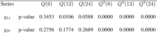
n
∑
t=1+j
w∗tε˜∗tε˜∗t−j.
Define the bootstrapped process∆n(λ) = ˜Sn∗(λ)−S˜n(λ)−Z˜n(λ), where 170
˜ Zn(λ) =
n−1
∑
j=1
1 √ n
n
∑
t=1+j
[(wt∗−1)˜γ(j)]
ψj(λ). (6)
4. Computer the bootstrapped test statisticCM˜ ∗n=∫π
0 {∆n(λ)} 2dλ.
5. Repeat steps 2-4 J times and denote by CM˜ ∗n,α the empirical 100(1−α)%sample per-centile ofCM˜ ∗nbased onJ bootstrapped values. Then we rejectH0at the significance levelαif
˜
CMn>CM˜ ∗n,α. 175
Particularly, when p=q= 0, we set ε˜t= ˜ε∗t =yt for all t in step 2. We now offer some remarks on the BRW method. First, the BRW is a natural extension of the RW method in Jin, Ying, and Wei (2001). The RW method as a variant of the traditional wild bootstrap in Wu (1986) has been widely used for statistical inference in regression based on the least absolute deviation estimation; see, e.g., Chen, Ying, Zhang, and Zhao (2008) and Chen, Guo, Lin, and 180
Ying (2010). However, from the proofs in the Appendix, we find that when εt is non-MDS, the original RW method (i.e.,bn= 1) is no longer applicable. To capture the dependence of εt beyond MDS, a block technique is necessary; see, e.g., Romano and Thombs (1996), Horowitz, Lobato, Nankervis, and Savin (2006), and Shao (2011a). Second,Z˜n(λ)in (6) is related to the termE{Sˇn(λ)}in Theorem 1, and it is a centering factor according to Shao (2011a). 185
Letdωbe any metric that metricizes weak convergence inL2[0, π], andL(ξn|χn)be the distri-bution of any random variableξngiven the sampleχn=:{y1,· · · , yn}; see Politis and Romano (1994). Denote byP∗,E∗andvar∗the probability, expectation and variance conditional onχn; by o∗
p(1)(O∗p(1)) a sequence of random variables converging to zero (bounded) in probability conditional onχn. We now are ready to present our second main result: 190
THEOREM2. Assume that (a) Assumptions1-3hold; (b)E|yt|8+4ν <∞for someν >0and
limk→∞k2[αy(k)]ν/(2+ν)= 0; (c)bn−1 =o(1)andbn=o(n1/3). Then, asn→ ∞,
(i) dω[L {∆n(λ)|χn},L {S(λ)}]→p 0;
(ii) consequently,
˜ CM∗n→d
∫ π
0
S2(λ)dλ in probability.
Remark5. Whenαy(k)decays exponentially, the condition forαy(k)in Theorem 2 is auto-matically satisfied.
price we pay for not assuming a stronger cumulant summability condition:
∞
∑
s1,···,sK=−∞
|sk||cum(y0, ys1· · · , ysK)|<∞, k = 1,· · · , K, (7)
forK = 1,· · · ,7. Note that (7) is implied by the GMC(8)condition ofytas shown in Wu and Shao (2004). If (7) holds, following a similar proof in Shao (2011a, p.221-222), we can easily show that Theorem 2 holds under some weaker conditions. We summarize it in the following
200
theorem:
THEOREM3. Assume that (a) Assumptions1-3and (7) hold; (b)Eyt8<∞; (c)b−n1 =o(1) and(logn)bn=o(n). Then, the conclusions in Theorem2hold.
Remark6. By a repetitive but even simple proof as in the Appendix, we can show that Theo-rems 2-3 hold ifbn= 1whenεtis an MDS.
205
Theorems 2-3 guarantee that whenJis large, the test statisticCM˜ nalong with its bootstrapped critical values has the correct asymptotic levels, is consistent in detectingH1, and has nontrivial local power to detectH1nif Assumption 4 holds.
Finally, it is worth noting that Theorem 2 requires a stronger condition forbnthan Theorem 3. This demonstrates that if we allow for a more general structure of yt, we may suffer from
210
a smaller valid range of bn. Hence, there is a tradeoff between the dependence structure ofyt and the theoretical valid range ofbn. Nevertheless, how to select the optimalbn under certain “criterion” is unknown up to now. This is a familiar problem with all blocking methods. The heuristic work in Hall, Horowitz, and Jing (1995) and Plolitis, Romano, and Wolf (1999) may be extended in this case, and we leave it for future study.
215
4. SIMULATION STUDIES
In this section, we examine the finite-sample performance ofCM˜ n for several weak ARMA models. As a comparison, we also consider the kernel-based testTnin Shao (2011b) (see also Hong (1996)), where
Tn= n−1
∑
j=1
K2
(
j mn
)
˜ ρ2(j),
withρ(j) = ˜˜ γ(j)/˜γ(0)being the residual autocorrelation at lagj,K(·)being the kernel func-tion satisfying Assumpfunc-tion 2.1 in Shao (2011b), andmnbeing the bandwidth such thatlogn=
o(mn)andmn=o(n1/2). UnderH0, Shao (2011b) showed that
nTn−mnC(K)
√
2mnD(K)
→dN(0,1) asn→ ∞,
whereC(K) =∫∞
0 K2(x)dxandD(K) =
∫∞
0 K4(x)dx. So, we rejectH0at significance level
α, ifTn> n−1
[√
2mnD(K)cα+mnC(K)
]
forn= 400and3,7,15,31,63forn= 1000. Here,δtis employed from the following Bernoulli distribution:
P
(
δt=
3−√5 2
)
= 1 + √
5 2√5 andP
(
δt=
3 +√5 2
)
= 1−1 + √
5 2√5 ,
although other choices like the standard exponential distribution are also suitable forδt. ForTn,
we use the Parzen kernelK(x)defined as 220
K(x) =
1−6x2+ 6|x|3 for0≤ |x| ≤1/2,
2(1− |x|)3 for1/2≤ |x| ≤1,
0 otherwise.
In general, since there is no clear objective procedure for optimally choosing the bandwidthmn, we carry out the calculation formn= 2,· · · ,20whenn= 400and2,· · ·,32whenn= 1000. In most cases ofmn, we find that the sizes ofTnare distorted (see Figure 1 below). Hence, only the results in which the sizes are close to their nominal ones are reported. 225
Example1. Consider the following weak ARMA(1,1) model:
yt=κyt−1+ 0.8εt−1+εt and εt=ηt2ηt−1, (8) whereηtis a sequence of iid N(0,1) random variables, andκ∈ {0.0,0.1,0.2,0.3,0.4}. Clearly,
εt in (8) are uncorrelated but non-MDS. Next, we use CM˜ n andTnto detect whether a weak MA(1) model is adequate to fit the data sample generated from model (8). The empirical power 230
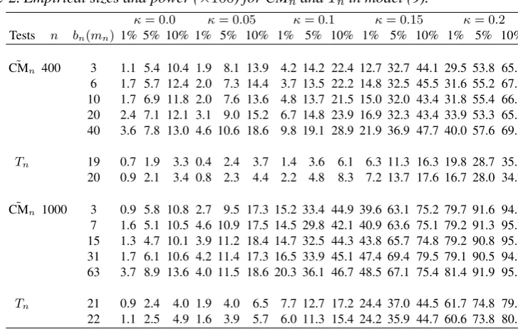
and sizes of both tests are reported in Table 1, and the sizes correspond to the cases thatκ= 0.0.
Example2. Consider the following switching-regime Markov model (see, e.g., Hamilton (1994)):
yt=κyt−1+ηt+ (0.2 + 0.3∆t)ηt−1, (9) where∆tis a sequence of Bernoulli random variables withP(∆t= 0) = 1/3andP(∆t= 1) = 235 2/3, ηtis a sequence of iid N(0,1) random variables, and κ∈ {0.0,0.05,0.1,0.15,0.2}. Here, we assume that∆tandηtare independent. Whenκ= 0.0, Francq and Zako¨ıan (1998) showed that model (9) admits a weak MA(1) representation:yt=εt+ϕεt−1, whereεtare uncorrelated but non-MDS. Thus, we can useCM˜ nandTnto detect whether a weak MA(1) model is adequate to fit the data sample generated from model (9). The empirical power and sizes of both tests are 240
reported in Table 2, and the sizes correspond to the cases thatκ= 0.0.
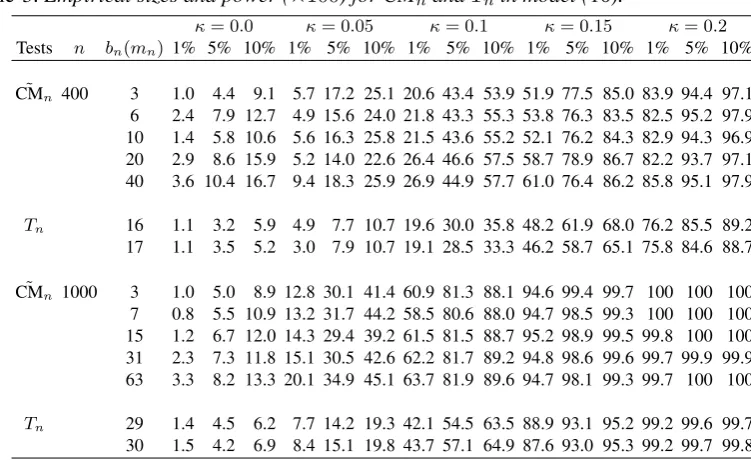
Example3. Consider the following bilinear model (see, e.g., Granger and Andersen (1978) and Pham (1986)):
yt=κηt−1+ηt+ 0.2yt−1ηt−2, (10) whereηtis a sequence of iid N(0,1) random variables, andκ∈ {0.0,0.05,0.1,0.15,0.2}. When 245 κ= 0.0, Francq and Zako¨ıan (1998) showed that model (10) admits a weak MA(3) representa-tion:yt=εt+ϕεt−3, whereεtare uncorrelated but non-MDS. Thus, we can useCMn˜ andTn to detect whether a weak MA(3) model is adequate to fit the data sample generated from model (10). The empirical power and sizes of both tests are reported in Table 3, and the sizes correspond
to the cases thatκ= 0.0. 250
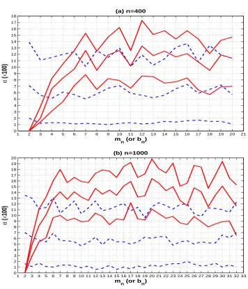
1 2 3 4 5 6 7 8 9 10 11 12 13 14 15 16 17 18 19 20 21 0
1 2 3 4 5 6 7 8 9 10 11 12 13 14 15 16 17 18
(a) n=400
m
n (or bn)
α
(
×
100)
1 2 3 4 5 6 7 8 9 10 11 12 13 14 15 16 17 18 19 20 21 22 23 24 25 26 27 28 29 30 31 32 33 0
1 2 3 4 5 6 7 8 9 10 11 12 13 14 15 16 17 18 19 20
(b) n=1000
m
n (or bn)
α
(
×
[image:11.595.107.464.90.506.2]100)
Fig. 1. The solid (or dashed) lines from top to bottom are the sizes ofTn(orCM˜ n) at the significance levelα=
10%,5%and1%in model (8) withκ= 0.0, based on different values ofmn(orbn).
For Tn, we find that its size performance is very sensitive to the choice of mn in model (8). A visual understanding of this phenomenon can be obtained in Figure 1, where we plot all the
255
empirical sizes ofTnfor different choices ofmn. As a comparison, the empirical sizes ofCM˜ n for different choices ofbnare also plotted in Figure 1. It is clear that whenmnis larger, the sizes ofTnare seriously distorted at each significance levelα, and whenmnis small,Tntends to be seriously undersized at significance levelsα= 5%and10%. This drawback ofTnis unchanged even when nbecomes larger. By using other kernels (e.g., the Bartlett kernel and the quadratic
260
spectral kernel), the similar result holds forTn, and hence they are not reported. Compared toTn, the sizes ofCM˜ nare much more robust at each significance level especially whenbnis small.
Furthermore, it is worth noting that unlike model (8),Tn is always undersized for different choices ofmnin models (9)-(10). This problem becomes extremely serious whenmnis small. However, like model (8), the size performance ofCM˜ nis much more robust in those cases. More
Table 1.Empirical sizes and power (×100) forCM˜ nandTnin model (8).
κ= 0.0 κ= 0.1 κ= 0.2 κ= 0.3 κ= 0.4
Tests n bn(mn) 1% 5% 10% 1% 5% 10% 1% 5% 10% 1% 5% 10% 1% 5% 10%
˜
CMn 400 3 1.3 6.8 12.5 3.9 14.1 26.0 22.0 49.0 64.4 54.9 80.2 89.1 80.1 93.7 96.8
6 1.1 5.5 11.5 3.3 14.0 26.5 19.9 44.1 59.7 50.2 77.8 87.3 73.2 91.2 95.5 10 1.6 5.5 10.9 4.2 15.3 27.1 22.0 47.3 60.7 49.6 75.6 87.1 68.6 88.0 95.6 20 1.3 6.6 13.3 5.4 17.1 26.2 21.8 46.8 59.7 47.9 72.4 82.7 64.9 85.7 93.7 40 3.2 7.8 13.3 8.4 16.8 25.0 25.1 44.3 56.4 48.5 68.4 80.1 63.8 80.5 89.9
Tn 3 1.4 2.0 3.8 8.9 12.9 16.6 37.4 46.5 52.1 80.2 86.0 89.3 97.1 98.3 98.6
4 3.1 6.6 8.2 15.5 20.7 24.6 53.8 61.4 65.8 88.4 91.2 92.9 98.1 99.0 99.5
˜
CMn 1000 3 1.2 5.1 11.6 13.2 35.6 48.1 63.8 82.7 88.8 94.4 98.4 99.2 99.1 99.8 99.9
7 1.0 4.3 9.3 13.9 31.9 46.0 60.1 82.1 89.6 93.5 97.8 99.2 98.9 99.8 99.9 15 1.2 5.3 11.8 13.8 33.4 44.8 62.6 82.7 90.5 91.5 97.8 99.0 97.9 99.7 99.8 31 0.9 6.2 12.5 13.2 34.3 47.9 62.9 83.9 91.1 90.2 98.7 99.7 94.6 99.2 99.8 63 2.1 6.3 11.7 17.1 31.6 46.2 65.7 82.3 88.4 86.5 95.8 97.9 88.5 96.6 99.0
Tn 3 2.9 4.9 6.2 21.5 30.2 35.5 79.3 84.1 86.7 98.9 99.5 99.7 100 100 100
4 5.4 8.2 11.1 33.0 41.2 46.2 87.3 91.2 92.6 99.9 100 100 100 100 100
Table 2.Empirical sizes and power (×100) forCM˜ nandTnin model (9).
κ= 0.0 κ= 0.05 κ= 0.1 κ= 0.15 κ= 0.2
Tests n bn(mn) 1% 5% 10% 1% 5% 10% 1% 5% 10% 1% 5% 10% 1% 5% 10%
˜
CMn 400 3 1.1 5.4 10.4 1.9 8.1 13.9 4.2 14.2 22.4 12.7 32.7 44.1 29.5 53.8 65.6
6 1.7 5.7 12.4 2.0 7.3 14.4 3.7 13.5 22.2 14.8 32.5 45.5 31.6 55.2 67.9 10 1.7 6.9 11.8 2.0 7.6 13.6 4.8 13.7 21.5 15.0 32.0 43.4 31.8 55.4 66.8 20 2.4 7.1 12.1 3.1 9.0 15.2 6.7 14.8 23.9 16.9 32.3 43.4 33.9 53.3 65.3 40 3.6 7.8 13.0 4.6 10.6 18.6 9.8 19.1 28.9 21.9 36.9 47.7 40.0 57.6 69.5
Tn 19 0.7 1.9 3.3 0.4 2.4 3.7 1.4 3.6 6.1 6.3 11.3 16.3 19.8 28.7 35.5
20 0.9 2.1 3.4 0.8 2.3 4.4 2.2 4.8 8.3 7.2 13.7 17.6 16.7 28.0 34.7
˜
CMn 1000 3 0.9 5.8 10.8 2.7 9.5 17.3 15.2 33.4 44.9 39.6 63.1 75.2 79.7 91.6 94.9
7 1.6 5.1 10.5 4.6 10.9 17.5 14.5 29.8 42.1 40.9 63.6 75.1 79.2 91.3 95.7 15 1.3 4.7 10.1 3.9 11.2 18.4 14.7 32.5 44.3 43.8 65.7 74.8 79.2 90.8 95.1 31 1.7 6.1 10.6 4.2 11.4 17.3 16.5 33.9 45.1 47.4 69.4 79.5 79.1 90.5 94.7 63 3.7 8.9 13.6 4.0 11.5 18.6 20.3 36.1 46.7 48.5 67.1 75.4 81.4 91.9 95.5
Tn 21 0.9 2.4 4.0 1.9 4.0 6.5 7.7 12.7 17.2 24.4 37.0 44.5 61.7 74.8 79.6
22 1.1 2.5 4.9 1.6 3.9 5.7 6.0 11.3 15.4 24.2 35.9 44.7 60.6 73.8 80.6
visual figures in this context, including the use of other kernels, are available from the authors on request. Overall, we know that the sizes ofCMn˜ are precise especially whenbnis small, while the sizes ofTn could be seriously undersized or oversized in most cases ofmn. It means that the performance ofTn is heavily relied on whether we can obtain an optimal mn, but this is not the case forCM˜ n. Considering the difficulty of selecting the optimal bandwidth in most of 270
[image:12.595.118.482.361.595.2]Table 3.Empirical sizes and power (×100) forCM˜ nandTnin model (10).
κ= 0.0 κ= 0.05 κ= 0.1 κ= 0.15 κ= 0.2
Tests n bn(mn) 1% 5% 10% 1% 5% 10% 1% 5% 10% 1% 5% 10% 1% 5% 10%
˜
CMn 400 3 1.0 4.4 9.1 5.7 17.2 25.1 20.6 43.4 53.9 51.9 77.5 85.0 83.9 94.4 97.1
6 2.4 7.9 12.7 4.9 15.6 24.0 21.8 43.3 55.3 53.8 76.3 83.5 82.5 95.2 97.9 10 1.4 5.8 10.6 5.6 16.3 25.8 21.5 43.6 55.2 52.1 76.2 84.3 82.9 94.3 96.9 20 2.9 8.6 15.9 5.2 14.0 22.6 26.4 46.6 57.5 58.7 78.9 86.7 82.2 93.7 97.1 40 3.6 10.4 16.7 9.4 18.3 25.9 26.9 44.9 57.7 61.0 76.4 86.2 85.8 95.1 97.9
Tn 16 1.1 3.2 5.9 4.9 7.7 10.7 19.6 30.0 35.8 48.2 61.9 68.0 76.2 85.5 89.2
17 1.1 3.5 5.2 3.0 7.9 10.7 19.1 28.5 33.3 46.2 58.7 65.1 75.8 84.6 88.7
˜
CMn 1000 3 1.0 5.0 8.9 12.8 30.1 41.4 60.9 81.3 88.1 94.6 99.4 99.7 100 100 100
7 0.8 5.5 10.9 13.2 31.7 44.2 58.5 80.6 88.0 94.7 98.5 99.3 100 100 100 15 1.2 6.7 12.0 14.3 29.4 39.2 61.5 81.5 88.7 95.2 98.9 99.5 99.8 100 100 31 2.3 7.3 11.8 15.1 30.5 42.6 62.2 81.7 89.2 94.8 98.6 99.6 99.7 99.9 99.9 63 3.3 8.2 13.3 20.1 34.9 45.1 63.7 81.9 89.6 94.7 98.1 99.3 99.7 100 100
Tn 29 1.4 4.5 6.2 7.7 14.2 19.3 42.1 54.5 63.5 88.9 93.1 95.2 99.2 99.6 99.7
30 1.5 4.2 6.9 8.4 15.1 19.8 43.7 57.1 64.9 87.6 93.0 95.3 99.2 99.7 99.8
powerful than Tn for all examined alternatives in models (9)-(10), while Tn has a power ad-vantage overCM˜ nfor all examined alternatives in model (8), except the cases thatmn= 3and
275
κ= 0.1. Thus, the performances ofCM˜ n andTn in finite sample are competitive in terms of power. Overall, althoughCM˜ ndoes not have a consistent power advantage overTn, it is reason-able to recommendCMn˜ in practice since it has a very robust size performance especially when the block size is small.
5. APPLICATION TOS&P 500STOCK INDEX
280
In this section, we revisit the real example on S&P 500 stock index in Escanciano and Velasco (2006). We consider two sample periods for the S&P 500 stock index. The first period is from 3 January 1994 until 31 December 1997 with a total of 1011 observations. The second period is from 2 January 1998 until 28 August 2002 with a total of 1170 observations. Denote the log-return of both series (after mean-adjusted) byy1tandy2t, respectively. The generalized spectral
285
tests in Escanciano and Velasco (2006, p.172) indicate thaty1t is non-MDS at the significance levelα= 5%, whiley2tis non-MDS at the significance levelα= 10%. Thus, we are of interest to test whethery1tory2tis a weak white noise (i.e., an uncorrelated sequence) by usingCMn. As˜ in Section 4, we choosebn=n1/5,2n1/5,√n/2,√nor2√n, and it deliversbn= 3,7,15,31for
y1tand4,8,16,32fory2t. The corresponding results forCM˜ nare listed in Table 4, from which
290
we can not reject the hypothesis thaty1tory2tis a weak white noise at the 5% significance level, and this conclusion is unchanged for all choices of bn. Thus, a weak but non-MDS processes should be suitable to fity1tory2t.
Next, we use CM˜ n to check whether a weak MA(3) model defined as yt=εt+ϕεt−3 for
|ϕ|<1, is adequate to fity1tory2t. Based on LS estimation, the fitted weak MA(3) models for 295
y1tandy2tare as follows:
y1t=ε1t−0.0482ε1t−3, (11)
Table 4.p-values ofCM˜ nfor testing the adequacy of a weak white noise on two S&P 500 stock
indexes
bn
Series n1/5
2n1/5 √n/2 √n 2√n
y1t p-value† 0.6900 0.6537 0.5050 0.6257 0.5637
y2t p-value 0.5110 0.5180 0.4017 0.4157 0.2783
†
p-values bootstrapped by the BRW method withJ= 3000.
where the estimated values ofσε21 = 6.2×10
−5 andσ2
ε2 = 1.8×10
−4. The p-values of CM˜ n in Table 5 indicate that models (11)-(12) are adequate at the 5% significance level, while thep- 300
values of the Ljung-Box test statisticsQ(M)and Li-Mak test statisticsQ2(M)in Table 6 imply that models (11)-(12) are not strong at the same significance level. Note that a Bilinear model like (10) withκ= 0has a weak MA(3) representation. Thus, it motivates us to fity1tory2tby the following Bilinear-GARCH model:
{
yt=ηt+uyt−1ηt−2,
ηt=√htνt and ht=ω+αηt2−1+βht−1, (13) 305
where|u|<1,ω >0,α, β≥0andνtis an iid re-scaled error sequence. For each series, model (13) is estimated by using the QMLE method (see, e.g, Ling (2007) and Francq and Zako¨ıan (2010)). The related results are summarized in Table 7, from which we know that model (13) is adequate to fity2t, while a marginal autocorrelation up to lag 6 is detected in the fitted conditional mean model fory1t. Based on this, we re-fity1tby another Bilinear-GARCH model: 310
{
yt=vηt−1+ηt+uyt−1ηt−2,
ηt=√htνt and ht=ω+αηt2−1+βht−1, (14)
where|v|<1,|u|<1,ω >0, α, β≥0 andνt is an iid re-scaled error sequence. The related results for the fitted model (14) are given in Table 7, from which we know that model (14) is adequate in fittingy1t.
Table 5.p-values ofCM˜ nfor testing the adequacy of a weak MA(3) model on two S&P 500 stock
indexes
bn
Series n1/5
2n1/5 √
n/2 √n 2√n y1t p-value† 0.9087 0.8923 0.8637 0.9707 0.9627
y2t p-value 0.8420 0.8630 0.6720 0.5560 0.4940
†
Table 6. p-values ofQ(M)andQ2(M) for testing the adequacy of a strong MA(3) model on two S&P 500 stock indexes
Series Q(6) Q(12) Q(24) Q2 (6) Q2
(12) Q2 (24) y1t p-value 0.3453 0.0106 0.0588 0.0000 0.0000 0.0000
y2t p-value 0.2756 0.1774 0.2689 0.0000 0.0000 0.0000
Table 7. QMLE-fitted model and its corresponding portmanteau tests on two S&P 500 stock indexes
QM LE
Series vn un ωn αn βn σ
2
ν Q(6) Q(24) Q
2 (6) Q2
(24)† Model (13) y1t − − − 0.9961 0.0000 0.1045 0.8686 0.9984 0.0461 0.2591 0.9517 0.9945
y2t − − − 0.8004 0.0000 0.1129 0.8213 0.9984 0.4106 0.3525 0.2549 0.6193
Model (14) y1t 0.0703 0.8001 0.0000 0.1083 0.8650 0.9971 0.4310 0.6353 0.9614 0.9951
†
p-values for the Ljung-Box test statisticsQ(6)andQ(24), and the Li-Mak test statisticsQ2
(6)andQ2 (24).
6. CONCLUDING REMARKS
315
In this paper, we study the asymptotic property of a CM-type spectral test statisticCM˜ n for checking the adequacy of an ARMA model with uncorrelated errors. By releasing the martingale difference assumption on the error terms, CM˜ n is applicable to a large class of uncorrelated nonlinear processes. Since we do not specify the form of error terms, the limiting distribution of CM˜ n is not pivotal, and so a BRW method is necessary to bootstrap the critical values of
320 ˜
CMn. Simulation studies show that the size and power performances ofCM˜ nare robust to the selection of block sizebnin BRW method especially when the sample size is large, while the size of kernel-based testTnin Shao (2011b) is always sensitive to the choice of the bandwidthmn. In addition, CMn˜ has a power advantage overTn under most of the examined alternatives. By revisiting two S&P 500 stock index series in Escanciano and Velasco (2006),CM˜ nsuggests that
325
the Bilinear-GARCH models are adequate to fit both series. This empirical example illustrates that although some economic or financial series is not a martingale difference sequence, it is still very likely to be an uncorrelated sequence. Our test statistic CM˜ n now gives us a way to check for the adequacy of ARMA models driven by an uncorrelated error sequence. Moreover, once a weak ARMA model is found to be adequate in fitting the given series, some non-linear
330
processes with a weak ARMA representation may also be considered to fit this series adequately. This point of view should be important for practitioners.
ACKNOWLEDGEMENT
This work is supported by Research Grants Council of the Hong Kong SAR Government, GRF grant HKU703711P, and National Natural Science Foundation of China (No.11201459).
APPENDIX: PROOFS
Denote byWh(j) =∫ π
0 h(λ)ψj(λ)dλfor anyh∈L2[0, π]; byPj = ∫π
0 ψ 2
j(λ)dλforj∈ N; byCa
positive generic constant which may vary from place to place. Note thatPj≤Cj−2uniformly inj∈ N,
and∫0πψj(λ)ψk(λ)dλ= 0whenj̸=kandj, k∈ N. In order to prove Theorem 1, we rewrite
˜ Sn(λ) =
[
˜
Sn(λ)−S˘n(λ)
]
+ ˘Sn(λ) 340
=[S˜n(λ)−S˘n(λ)
]
+[S˘n(λ)−Sˇn(λ)
]
+ ˇSn(λ)
=I1n(λ) +I2n(λ) + ˇSn(λ)say. (A1)
where S˘n(λ) =∑n−j=11
√nγ˘(j)ψ
j(λ) with ˘γ(j) =n−1∑nt=1+|j|ε˘tε˘t−|j| and ε˘t=εt(θn). Then, we
need the following four lemmas:
LEMMA A1. Suppose that Assumptions 1-2 hold. Then,∥I1n(λ)∥2=op(1). 345
Proof. By a direct calculation, we have
E∥I1n(λ)∥2=
1 n
n−1 ∑
j=1
E
n
∑
t=1+j
btj(θn)
2
Pj,
wherebtj(θ) =εt(θ)εt−j(θ)−ε˜t(θ)˜εt−j(θ). By Minkowski inequality, it follows that
E∥I1n(λ)∥2≤
1 n
n−1 ∑
j=1
n
∑
t=1+j
{
E[btj(θn)]2
}1/2 2
Pj
≤ 1n
n−1 ∑
j=1
n
∑
t=1+j
{
E
[
sup
Θ ∥
btj(θ)∥
]2}1/2 2
Pj. (A2) 350
By Lemmas A.1 and A.4 in Ling (2007), we know that there exists a constantρ∈(0,1)such that sup
Θ ∥
btj(θ)∥ ≤sup
Θ ∥
[εt(θ)−ε˜t(θ)]εt−j(θ)∥+ sup
Θ ∥
˜
εt(θ) [εt−j(θ)−ε˜t−j(θ)]∥
≤O(ρt)ξρ0ξρt−j+O(ρt−j)ξρ0ξρt,
whereξρt= 1 +∑∞i=0ρi|yt−i|. Note thatE|ξρt|4<∞by Assumption 2. Thus, from (A2), by H¨older
inequality, we can show that 355
E∥I1n(λ)∥2≤ 1
n
n−1 ∑
j=1
n
∑
t=1+j
{
O(ρ2t)E[ξρ0ξρt−j]2+O(ρ2(t−j))E[ξρ0ξρt]2
}1/2 2
Pj
≤n1
n−1 ∑
j=1
n
∑
t=1+j
{
O(ρ2t)(E[ξρ0]4E[ξρt−j]4
)1/2
+O(ρ2(t−j))(E[ξρ0]4E[ξρt]4
)1/2}1/2 )2
Pj
≤n1
n−1 ∑
j=1
n
∑
t=1+j
{
O(ρt) +O(ρt−j)} 2
Pj
=O(n−1), 360
LEMMA A2. Suppose that Assumptions 1-3 hold. Then,
(i) E
[
∂lt(ˇθ0)
∂θ
]
= 0;
(ii) √n(θn−θˇ0) =Op(1)with√n(θn−θˇ0) =−Σ−1 [ 1 √n n ∑ t=1
∂lt(ˇθ0)
∂θ
]
+op(1).
365
Proof. (i) By Assumption 1, it is not hard to show that
sup Θ 1 √n n ∑ t=1 [
∂lt(θ)
∂θ −
∂˜lt(θ)
∂θ ]
=op(1), (A3)
sup Θ 1 n n ∑ t=1 [
∂2lt(θ)
∂θ∂θ′ −
∂2˜lt(θ)
∂θ∂θ′ ]
=op(1). (A4)
Then, since∂˜lt(θn)/∂θ= 0, by Taylor’s expansion and (A3)-(A4), we have
θn−θˇ0=− [ 1 n n ∑ t=1
∂2˜l
t(ξn)
∂θ∂θ′
]−1[
1 n
n
∑
t=1
∂˜lt(ˇθ0)
∂θ ] 370 =− [ 1 n n ∑ t=1
∂2l
t(ξn)
∂θ∂θ′
]−1[
1 n
n
∑
t=1
∂lt(ˇθ0)
∂θ
]
+op(1), (A5)
whereξnlies betweenθnandθˇ0. By Lemma A.1 in Ling (2007), we know that
Esup Θ
∂2l
t(θ)
∂θ∂θ′
≤
CEξρt−2 1<∞
for someρ∈(0,1), where the last inequality follows from Assumption 2. Thus, by Theorem 3.1 in Ling and McAeer (2003), we have
1 n
n
∑
t=1
∂2l
t(ξn)
∂θ∂θ′ =E
[∂2l
t(ξn)
∂θ∂θ′
]
+op(1) = Σ +op(1), (A6)
where the last equality holds by the dominated convergence theorem and the fact thatξn →pθˇ0asn→ ∞
375
by Assumption 3. By (A5)-(A6) and the ergodic theorem, it follows that
θn−θˇ0=−Σ−1 [ 1 n n ∑ t=1
∂lt(ˇθ0)
∂θ
]
+op(1) =−Σ−1E
[
∂lt(ˇθ0)
∂θ
]
+op(1).
Sinceθn−θˇ0=op(1)by Assumption 3, it implies that (i) holds.
(ii) By (A3)-(A5), it is not hard to see that
√n(θ
n−θˇ0) =− [ 1 n n ∑ t=1
∂2l
t(ξn)
∂θ∂θ′
]−1[
1
√n
n
∑
t=1
∂lt(ˇθ0)
∂θ
]
+op(1). 380
Note that ∂lt(ˇθ0)/∂θ= 2ˇεt(∂εˇt/∂θ). Thus, by Assumptions 1 and 2(i), Lemmas 3-4 in Francq and
Zako¨ıan (1998) implies thatn−1/2∑n
t=1∂lt(ˇθ0)/∂θ=Op(1). By (A6), it follows that (ii) holds.
LEMMA A3. Suppose that Assumptions 1-3 hold. Then,
∥I2n(λ)−Wn′(λ)[
√
where
Wn(λ) = n−1 ∑
j=1
E
[
∂(ˇεtεˇt−j)
∂θ
]
ψj(λ).
385
Proof. By Taylor’s expansion, we haveε˘t−εˇt= (∂εt(ξn)/θ′)(θn−θˇ0), where ξn lies betweenθn
andθˇ0. Then, it follows that
I2n(λ) = n−1 ∑ j=1 1 n n ∑
t=1+j
[∂ε
t(ξn)
∂θ′ ε˘t−j+ ˇεt
∂εt−j(ξn)
∂θ′
]
ψj(λ)
[√n(θn−θˇ0)],
which entails
I2n(λ) =
{
I2(1)n(λ, ξn, θn) +I2(2)n(λ, ξn) +I2(3)n(λ)
}
[√n(θn−θˇ0)], (A7) 390
where
I2(1)n(λ, θ1, θ2) =
n−1 ∑ j=1 1 n n ∑
t=1+j
[∂ε
t(θ1)
∂θ′ εt−j(θ2)−E
(∂εˇ
t
∂θ′εˇt−j
)]
ψj(λ)
,
I2(2)n(λ, θ1) =
n−1 ∑ j=1 1 n n ∑
t=1+j
[
ˇ εt
∂εt−j(θ1)
∂θ′ −E
(
ˇ εt
∂εˇt−j
∂θ′
)]
ψj(λ)
,
I2(3)n(λ) = n−1 ∑
j=1 {
n−j n
[
E
(
∂εˇt
∂θ′εˇt−j
)
+E
(
ˇ εt
∂εˇt−j
∂θ′
)]
ψj(λ)
}
.
We first considerI2(1)n(λ, ξn, θn). By a direct calculation, we have 395
E∥I2(1)n(λ, ξn, θn)∥2= n−1 ∑
j=1
(Ec2nj)Pj, (A8)
where
cnj =
1 n
n
∑
t=1+j
[
∂εt(ξn)
∂θ′ εt−j(θn)−E
(
∂εˇt
∂θ′εˇt−j
)]
.
Note that by Assumption 1 and Lemma A.1 in Ling (2007), we have
sup
Θ |
εt(θ)| ≤Cξρt and sup
Θ
εt(θ)
∂θ
≤
Cξρt−1
for someρ∈(0,1). Thus, as for (A6), by Assumptions 2 and 3(i), we can show that uniformly inj ∈
{1,· · · , n−1},Ec2
nj=o(1). Thus, since
∑∞
j=1Pj<∞, by (A8), it is straightforward to see that 400
E∥I2(1)n(λ, ξn, θn)∥2= n−1 ∑
j=1
o(Pj) =o(1),
which implies that∥I2(1)n(λ, ξn, θn)∥2=op(1). Similarly,∥I2(2)n(λ, ξn)∥2=op(1).
Next, we considerI2(3)n(λ). By a direct calculation and the factPj =O(j−2), we have
E∥I2(3)n(λ)−Wn(λ)∥2= n−1 ∑ j=1 j2 n2 [ E
(∂εˇ
t
∂θ′εˇt−j
)
+E
(
ˇ εt
∂εˇt−j
∂θ′
)]2
Pj =O(n−1).
LEMMA A4. Suppose that Assumptions 1-3 hold. Then, n−1 ∑ j=1 ( 1 √n j ∑ t=1 ztj )
ψj(λ)
2
=op(1),
whereztj is defined as in (4).
Proof. First, by Lemma A2(i), we haveEztj = 0. Then, as for (A6), by Assumptions 1-2, it is not hard
to show that
E [ 1 j j ∑ t=1 ztj ]2
→0 as j→ ∞.
Thus,∀ε >0, there exists an0(ε)such that whenj≥n0,
E [ 1 j j ∑ t=1 ztj ]2 < ε.
Next, by a direct calculation, forn≥max(n0+ 1,⌊ε−1⌋), we have
410 E n−1 ∑ j=1 ( 1 √n j ∑ t=1 ztj )
ψj(λ)
2 = 1 n n−1 ∑ j=1
j2E
[ 1 j j ∑ t=1 ztj ]2 Pj = 1 n
n0−1
∑
j=1
j2E
[ 1 j j ∑ t=1 ztj ]2
Pj+
1 n
n−1 ∑
j=n0
j2E
[ 1 j j ∑ t=1 ztj ]2 Pj ≤O (1 n ) + ε n n−1 ∑
j=n0
j2Pj
=O
(
1 n
)
+O(ε) =O(ε).
415
Thus, it follows that conclusion holds.
PROOF OF THEOREM 1. By (A1) and Lemmas A1, A3 and A4, it suffices to show thatS¯n(λ)−
E{S¯n(λ)} ⇒S(λ)asn→ ∞, whereS¯n(λ) =∑n−j=11√nλ¯(j)ψj(λ)withλ¯n(λ) =n−1∑nt=1+|j|et,j.
Here, we have used the fact thatE{Sˇn(λ)}=E{S¯n(λ)}by Lemma A.2(i). For each fixed integerK∈
{1,· · ·, n−1}, we rewrite
¯ Sn(λ) =
K
∑
j=1 √
n¯λ(j)ψj(λ) + n−1 ∑
j=K+1 √
nλ¯(j)ψj(λ) =: ¯SnK(λ) +RKn(λ).
Then, as in Shao (2011), the conclusion holds from the following three claims:
(a). For anyh∈L2[0, π], the finite dimensional distributions of⟨S¯nK−E( ¯SnK), h⟩converge to those
of⟨SK(λ), h
⟩, whereSK(λ)is a Gaussian process with zero mean and asymptotic projected variances
σh,K2 =var[⟨SK, h⟩] = K ∑ j=1 K ∑ k=1 ∞ ∑
d=−∞
cov(et,j, et−d,k)Wh(j)Wh(k). 420
(b). The sequence{S¯K
(c). For∀ε >0,limK→∞limn→∞P
( ∥RK
n(λ)−E{RKn(λ)}∥> ε
)
= 0. Q.E.D.
PROOF OF CLAIM(a). By a direct calculation, we can show that
⟨S¯Kn −E( ¯SnK), h⟩=
1
√n
K
∑
j=1
n
∑
t=j+1
{et,j−E(et,j)}Wh(j) 425
=√1 n
K+1 ∑
t=2
t−1 ∑
j=1
{et,j−E(et,j)}Wh(j)
+√1n
n
∑
t=K+2
K
∑
j=1
{et,j−E(et,j)}Wh(j), (A9)
where the first summand above isop(1)sinceKis finite. Rewrite
Yt=: K
∑
j=1
et,jWh(j) = 1′K+1× (
ˇ
εtεˇt−1Wh(1),· · ·,εˇtεˇt−KWh(K), κεˇt∂εˇt
∂θ′
)′
=: 1′
K+1×vt, (A10) 430
where1K+1= (1,· · ·,1)′ ∈ R(K+1)×1andκ=−2∑Kj=1E[∂(ˇεtεˇt−j)/∂θ′]Wh(j). By the finiteness
ofWh(j)andκand the same argument as in Francq, Roy, and Zako¨ıan (2005, page 243), we have
1
√
n
n
∑
t=K+2
(vt−Evt)→dN
(
0, var
[
1
√
n
n
∑
t=K+2
vt
])
asn→ ∞.
Hence, it follows that for the second summand, n−1/2∑n
t=K+2(Yt−EYt)→dN(0,Iˇ) as n→ ∞,
where
ˇ I= lim
n→∞var
(
1
√
n
n
∑
t=K+2
Yt
)
= lim
n→∞
1 n
K
∑
j=1
K
∑
k=1 ( n
∑
t=K+2
n
∑
t′=K+2
cov(et,j, et′,k)
)
Wh(j)Wh(k)
= lim
n→∞
1 n
K
∑
j=1
K
∑
k=1
n−K−2 ∑
d=K+2−n
n+min(0,d) ∑
t=K+2+max(0,d)
cov(et,j, et−d,k)
Wh(j)Wh(k) 435
= lim
n→∞ K
∑
j=1
K
∑
k=1
( n−K−2 ∑
d=K+2−n
n−K−2− |d|
n cov(et,j, et−d,k)
)
Wh(j)Wh(k)
=σ2
h,K. (A11)
Thus, it follows that claim (a) holds. Q.E.D.
PROOF OF CLAIM(b). First, as for (A9), we have 440
¯
SnK−E( ¯SnK) =
1
√n
K
∑
j=1
n
∑
t=j+1
{et,j−E(et,j)}ψj(λ)
= √1n
K+1 ∑
t=2
t−1 ∑
j=1
{et,j−E(et,j)}ψj(λ) +
1
√n
n
∑
t=K+2
where the first term in (A12) is tight since each summand is tight, and
GK t =
K
∑
j=1
{et,j−E(et,j)}ψj(λ).
Next, we use Theorem 2.1 in Politis and Romano (1994) to prove the tightness of the second term in (A12). Note thatGK
t is independent ton. We only need to verify that
(i)E∥GKt ∥2<∞; 445
(ii) lim
n→∞ n
∑
t=K+2
E[
⟨GKK+2, GKt ⟩
]
=
∞
∑
t=K+2
E[
⟨GKK+2, GKt ⟩
]
<∞, and the last series
converges absolutely;
(iii) lim
n→∞var
[
⟨S¯nK−E( ¯SnK), h⟩
]
→σh,K2 .
The proof of (i) is trivial, and the proof of (iii) is directly from the one as for (A11). We now consider the proof of (ii). Note that
450
∞
∑
t=K+2 E
[
⟨GKK+2, GKt ⟩
] =
∞
∑
t=K+2
K
∑
j=1
cov(et,j, eK+2,j)Pj
. (A13)
Using the same argument as for Lemma 3 in Francq and Zako¨ıan (1998), it is not hard to show that for eachj∈ {1,· · · , K}, there exists aρ∈(0,1)such that
|cov(et,j, eK+2,j)| ≤C
{
ρ|t−K−2|/2+
[
αy
(⌊
|t−K−2|
2
⌋)]ν/(2+ν)}
. (A14)
By (A13)-(A14), it follows that
455
∞
∑
t=K+2 E
[
⟨GKK+2, GKt ⟩
] ≤C
K
∑
j=1
Pj
∞
∑
s=0 {
ρ|s|/2+
[
αy
(⌊ |s|
2
⌋)]ν/(2+ν)}
<∞,
which implies that (ii) holds. This completes the proof of claim (b). Q.E.D.
PROOF OF CLAIM(c). First, by a direct calculation, we have
E∥RKn(λ)−E{RnK(λ)}∥2=
1 n
n−1 ∑
j=K+1
n
∑
t,t′=j+1
cov(et,j, et′,j)Pj. (A15) 460
Since et,j = ˇεtεˇt−j+ztj, there are four terms in cov(et,j, et′,j). For simplicity, we only prove the
conclusion for the term cov(ztj, zt′j), since the proofs for other terms are similar. Note that for any
m∈ {1,· · · , p+q}, them-th entry ofztj satisfies that
ztj,m=O(1)ˇεt∂εt(ˇθ0)
∂θm
=O(1)
[∞ ∑
i=0
ciyt−i
] [∞ ∑
k=0
ck,myt−k
]
whereci=O(ρi)andci,m =O(ρi)for someρ∈(0,1). Then, for any(m, m′)∈ {1,· · ·, p+q}2, we 465
have
1 n
n−1 ∑
j=K+1
n
∑
t,t′=j+1
cov(ztj,m, zt′j,m′)
≤O
(
1 n
) n−1 ∑
j=K+1
n
∑
t,t′=j+1 ∑
i,k,i′,k′≥0
|cick,m′ci′ck′,m′| |cov(yt−iyt−k, yt′−i′yt′−k′)|Pj
≤O(1) ∑
i,k,i′,k′≥0
|cick,m′ci′ck′,m′| n−1 ∑
j=K+1
1 n
n
∑
t,t′=j+1
|cov(y0yi−k, yt′−t+i−i′yt′−t+i−k′)|
Pj.
Furthermore, by Assumption 2, we can show that for anyi, k, i′, k′, j, 470
1 n
n
∑
t,t′=j+1
|cov(y0yi−k, yt′−t+i−i′yt′−t+i−k′)|
≤ 1n
n
∑
t,t′=j+1
{|cum(y0, yi−k, yt′−t+i−i′, yt′−t+i−k′)|
+|γ(t′−t+i−i′)γ(t′−t+k−k′)|+|γ(t′−t+i−k′)γ(t′−t+k−i′)|}
≤
n−1−j
∑
d=−(n−1−j)
n−1−j− |d|
n {|cum(y0, yi−k, yd+i−i′, yd+i−k′)|
+|γ(d+i−i′)γ(d+k−k′)|+|γ(d+i−k′)γ(d+k−i′)|} 475
≤
∞
∑
s1,s2,s3=−∞
|cum(y0, ys1, ys2, ys3)|+ 2
∞
∑
s=−∞
[γ(s)]2<∞.
Thus, it follows that
1 n
n−1 ∑
j=K+1
n
∑
t,t′=j+1
cov(ztj,m, zt′j,m′)≤O(1) ∞
∑
j=K+1
Pj→0asK→ ∞. (A17)
By (A15) and (A17), we know thatlimK→∞limn→∞E∥RKn(λ)−E{RKn(λ)}∥2= 0. Now, claim (c)
follows directly from Chebyshev’s inequality. Q.E.D. 480
PROOF OFCOROLLARY1. UnderH0, we haveθ0= ˇθ0, which implies thatE{Sˇn(λ)}= 0. Thus, (i)
follows directly from continuous mapping theorem. For (ii), sincen−1/2S˜
n(λ)−E
{
n−1/2Sˇ
n(λ)
} ⇒0 inL2[0, π]by Theorem 1, it follows that
˜ CMn
n =
∫ π 0
[
˜ Sn(λ)
√n ]2
dλ→p
∫ π 0
{
E
[Sˇ
n(λ)
√n ]}2
dλ=
∞
∑
j=1
[E(ˇεtεˇt−j)]2Pj
asn→ ∞, i.e., (ii) holds. Q.E.D.
PROOF OFCOROLLARY2. Rewrite
˜
Sn(λ) = ¯Sn(λ) +
[
˜
Sn(λ)−S¯n(λ)
]
485
=[¯
Sn(λ)−E{S¯n(λ)}]+E{S¯n(λ)}+
[
˜
Sn(λ)−S¯n(λ)
]
On one hand, by Assumptions 1-3, from the proof of Theorem 1, we have
¯
Sn(λ)−E{S¯n(λ)}⇒S(λ) and E∥S˜n(λ)−S¯n(λ)∥2→0 asn→ ∞. (A19)
On the other hand, sinceθˇ0=θ0by Assumption 4, we can show that underH1n,
E{¯
Sn(λ)}=E{Sˇn(λ)} 490 =E n−1 ∑ j=1 √
nγˆ(j)ψj(λ)
= n−1 ∑ j=1 √
nγn(j)ψj(λ)
= γ(0) 2π
n−1 ∑
j=1 [
g(ω)eijωdω]
ψj(λ)→
γ(0) 2π
∫ λ 0
g(ω)dω (A20)
asn→ ∞, whereγn(j)is defined as in (5). Now, the conclusion holds from (A18)-(A20) and continuous
mapping theorem. Q.E.D.
495
Next, in order to prove Theorem 2, we need three more lemmas:
LEMMA A5. Assume that Assumptions 1-3 hold andb−1
n =o(1). Then, (i)∥θ∗n−θˇ0∥=o∗p(1);
(ii)√n(θ∗
n−θˇ0) =O∗p(1), where√n(θ∗n−θˇ0) =−Σ−1
[
n−1/2∑n
t=1w∗t ∂lt(ˇθ0)
∂θ
]
+o∗ p(1).
Proof. As for (A5), by Assumptions 1-2, we can show that
500
θ∗n−θˇ0=− [ 1 n n ∑ t=1
∂2l∗ t(ξn)
∂θ∂θ′
]−1[
1 n n ∑ t=1 ∂l∗ t(ˇθ0)
∂θ
]
+op(1)
=− [ 1 n n ∑ t=1
w∗t
∂2l
t(ξn)
∂θ∂θ′
]−1[
1 n
n
∑
t=1
(wt∗−1)
∂lt(ˇθ0)
∂θ + 1 n n ∑ t=1
∂lt(ˇθ0)
∂θ
]
+op(1)
=:−[s1n]−1[s2n+s3n] +op(1),
whereξn lies between θ∗n andθˇ0. First, by Lemma A.4 in Ling (2007) and the ergodic theorem, it is
straightforward to see that
E∗
∥s1n∥ ≤
1 n
n
∑
t=1
E∗(w∗ t) sup
θ
∂2l
t(θ)
∂θ∂θ′ = 1 n n ∑ t=1 sup θ
∂2l
t(θ)
∂θ∂θ′
=Op(1),
which entailss1n =O∗p(1). Next, by a direct calculation and the stationarity oflt(θ), we have
E{E∗[s
2ns′2n]}=
1 n2 Ln ∑ s=1 E ∑
t,t′∈Bs ∂lt(ˇθ0)
∂θ
∂lt′(ˇθ0)
∂θ′
505
= bn n2 Ln ∑ s=1 var [ 1 √ bn ∑ t∈Bs ∂lt(ˇθ0)
∂θ
]
= bnLn n2 var
[ 1 √ bn bn ∑ t=1
∂lt(ˇθ0)
∂θ
]
Note thatb−1
n =o(1). By Lemma 3 in Francq and Zako¨ıan (1998), we know that
lim n→∞var [ 1 √ bn bn ∑ t=1
∂lt(ˇθ0)
∂θ
]
exists.
Thus, by (A21), it follows thatE{E∗[s
2ns′2n]}=O(n−1), which impliess2n =O∗p(n−1/2). Note that 510
s3n=op(1)by the ergodic theorem and Lemma A2(i). Thus, it follows that (i) holds.
For (ii), as for (A5), we have
√
n(θ∗n−θˇ0) =− [ 1 n n ∑ t=1
∂2l∗ t(ξn)
∂θ∂θ′
]−1[
1 √n n ∑ t=1 ∂l∗ t(ˇθ0)
∂θ
]
+op(1)
=−[s1n]−1[√ns2n+√ns3n]+op(1). (A22)
By (i), it is not hard to show that 515
1 n
n
∑
t=1
(w∗t −1)
∂2l
t(ξn)
∂θ∂θ′ =o ∗
p(1) and
1 n
n
∑
t=1
∂2l
t(ξn)
∂θ∂θ′ = Σ +o ∗ p(1).
Then, it follows thats1n= Σ +o∗p(1). Note that√ns2n=Op∗(1)and√ns3n=Op(1)by Lemma A2(ii).
Thus, by (A22), we know that (ii) holds.
LEMMA A6. Assume that Assumptions 1-3 hold,b−1
n =o(1), andbnn−1=o(1). Then,E∗∥Z˜n(γ)−
¯
Zn(γ)∥2=op(1), where 520
¯ Zn(γ) =
n−1 ∑ j=1 1 √n n ∑
t=1+j
(w∗
t −1)E(ˇεtεˇt−j)
ψj(λ).
Proof. Note that
E∗∥Z˜n(γ)−Z¯n(γ)∥2≤2E∗∥Z˜n(γ)−Zˇn(γ)∥2+ 2E∗∥Zˇn(γ)−Z¯n(γ)∥2, (A23)
where 525
ˇ Zn(γ) =
n−1 ∑ j=1 1 √ n n ∑
t=1+j
(w∗
t −1)(n−j)
n E(ˇεtεˇt−j)
ψj(λ).
By a direct calculation, we have
E∗∥Z˜n(γ)−Zˇn(γ)∥2= n−1 ∑ j=1 1 nE ∗ n ∑
t=1+j
(w∗t−1)dnj
2 Pj = n−1 ∑ j=1 1 n Ln ∑ s=1 ∑
t∈Bs∩[1+j,n] dnj 2 Pj ≤ n−1 ∑ j=1 {L
nb2n
n d
2
nj
}
Pj 530
=bn n
n−1 ∑
j=1 (√
ndnj)
2
wherednj =n−1∑nt′=1+j[˜εt′ε˜t′−j−E(ˇεt′εˇt′−j)]. By Lemma A.4 in Ling (2007), it is straightforward
to see that
√
ndnj = √1
n
n
∑
t=1+j
[˘εtε˘t−j−E(ˇεtεˇt−j)] +op(1). (A25)
Next, by Taylor’s expansion, we have
535
˘
εtε˘t−j= ˇεtεˇt−j+∂(ˇεtεˇt−j)
∂θ′ (θn−θˇ0) + (θn−θˇ0) ′
[
1 2
∂2(εt(θ)εt−j(θ))
∂θ∂θ′
θ=ξn
]
(θn−θˇ0),
whereξnlies betweenθn andθˇ0. Note that√n(θn−θˇ0) =Op(1)by Lemma A2(ii). Thus, by (A25) it
follows that for allj∈ {1,· · · , n−1},
√
ndnj =
1
√n
n
∑
t=1+j
[ˇεtεˇt−j−E(ˇεtεˇt−j)]
+1 n
n
∑
t=1+j
∂(ˇεtεˇt−j)
∂θ′ [
√
n(θn−θˇ0)] +op(1) 540
=√1n
n
∑
t=1+j
[ˇεtεˇt−j−E(ˇεtεˇt−j)] +Op(1). (A26)
As for (A17), we can show that for allj∈ {1,· · · , n−1},
E
1
√n
n
∑
t=1+j
[ˇεtεˇt−j−E(ˇεtεˇt−j)]
2
= 1 n
n
∑
t,t′=1+j
cov(ˇεtεˇt−j,εˇt′εˇt′−j) =O(1).
Thus, by (A26), we know that√ndnj=Op(1). Sincebnn−1=o(1)and∑∞j=1Pj <∞, by (A24), it
entails that
545
E∗
∥Z˜n(γ)−Zˇn(γ)∥2=
bn
n
n−1 ∑
j=1
Op(Pj) =op(1). (A27)
Next, sincebnn−1=o(1), it is straightforward to see that
E∗∥Zˇn(γ)−Z¯n(γ)∥2=E∗
n−1 ∑
j=1
j n3/2
n
∑
t=1+j
(w∗t−1)E(ˇεtεˇt−j)
ψj(λ)
2
=
n−1 ∑
j=1
j2
n3E
∗
n
∑
t=1+j
(w∗t−1)E(ˇεtεˇt−j)
2
Pj
=
n−1 ∑
j=1
j2
n3
Ln
∑
s=1
∑
t∈Bs∩[1+j,n]
E(ˇεtεˇt−j)
2
Pj 550
≤
n−1 ∑
j=1
j2
n3Lnb 2
nPj
=O(
bnn−1)=o(1). (A28)
LEMMA A7. Suppose that Assumptions 1-3 hold,b−1
n =o(1), and(logn)bnn−1=o(1). Then,
E∗ n−1 ∑ j=1 [ 1 √n j ∑ t=1
(w∗t −1)˜ztj
]
ψj(λ)
2
=op(1),
where˜ztjis defined in the same way asztj in (4) with˜lt(ˇθ0)replacinglt(ˇθ0).
Proof. By a direct calculation, we have 555
E∗ n−1 ∑ j=1 [ 1 √ n j ∑ t=1
(wt∗−1)˜ztj
]
ψj(λ)
2 = n−1 ∑ j=1 1 nE ∗ ( j ∑ t=1
(wt∗−1)˜ztj
)2 Pj = n−1 ∑ j=1 1 n Ln ∑ s=1 ∑
t∈Bs∩[1,j] ˜ ztj
2
Pj.
By Lemma A.4 in Ling (2007), it is straightforward to see that
n−1 ∑ j=1 1 n Ln ∑ s=1 ∑
t∈Bs∩[1,j] ˜ ztj
2
Pj= n−1 ∑ j=1 1 n Ln ∑ s=1 ∑
t∈Bs∩[1,j] ztj
2
Pj+op(1) =:Hn+op(1).
Note that∑∞
j=1Pj <∞. For∀ε >0, there exists aj0(ε)>0such that 560 ∞
∑
j=j0+1
Pj < ε.
Sincebn→ ∞asn→ ∞, we rewrite
Hn = j0 ∑ j=1 1 n Ln ∑ s=1 ∑
t∈Bs∩[1,j] ztj
2
Pj+ bn
∑
j=j0+1
1 n Ln ∑ s=1 ∑
t∈Bs∩[1,j] ztj 2 Pj + n−1 ∑
j=bn+1 1 n Ln ∑ s=1 ∑
t∈Bs∩[1,j] ztj
2
Pj
=:H1n+H2n+H3n. (A29) 565
First, forH1n, we know that asnis large enough,
EH1n≤ j0 ∑ j=1 1 n Ln ∑ s=1
O(j02)Pj =O
(L
n
n
)
< ε. (A30)
Next, forH2n, a direct calculation gives us that
H2n= bn
∑
j=j0+1
1 n 1 ∑ s=1 ∑
t∈Bs∩[1,j] ztj
2
Pj= bn
∑
j=j0+1
1 n ( ∑ t∈B1 ztj )2
By Lemma 3 in Francq and Zako¨ıan (1998), it follows that asnis large enough,
570
EH2n= bn
∑
j=j0+1
bn nE ( 1 √ bn bn ∑ t=1 ztj )2 Pj = bn ∑
j=j0+1
bn
nO(Pj)≤O
(b
n
nε
)
< ε. (A31)
Third, forH3n, we truncate it as
H3n =
1 n
Ln
∑
s′=2 ∑
j∈Bs′ Ln ∑ s=1 ∑
t∈Bs∩[1,j] ztj 2 Pj = 1 n Ln ∑
s′=2 ∑
j∈Bs′
( ∑
s<s′
+∑
s=s′
)
∑
t∈Bs∩[1,j] ztj
2
Pj. (A32)
575
As for (A31), by the stationarity ofztj, we can show that
E 1 n Ln ∑
s′=2 ∑
j∈Bs′
∑
s<s′
∑
t∈Bs∩[1,j] ztj 2 Pj = 1 n Ln ∑
s′=2 ∑
j∈Bs′
∑ s<s′ E ( ∑ t∈Bs ztj )2 Pj
=bn n
Ln
∑
s′=2
∑
j∈Bs′
∑
s<s′
O(Pj)
≤bnnLn
Ln
∑
s′=2 ∑
j∈Bs′
O(Pj)
≤
∞
∑
j=j0+1
O(Pj)< ε. (A33)
580
Furthermore, since(logn)bnn−1=o(1), it is not hard to see that
E 1 n Ln ∑
s′=2 ∑
j∈Bs′
∑
s=s′
∑
t∈Bs∩[1,j] ztj 2 Pj = 1 n Ln ∑
s′=2 ∑
j∈Bs′
O(b2n)Pj
= 1 n
n−1 ∑
j=bn+1 O(b2n)
1 j2
≤ bnn
n−1 ∑
j=bn+1 O(1)1
j
=O
(b
nlogn
n
)
< ε. (A34)
585
Now, the conclusion follows from (A29)-(A34).
PROOF OFTHEOREM2. By Taylor’s expansion we have
˜
ε∗tε˜∗t−j= ˜εtε˜t−j+
∂(˜εtε˜t−j)
∂θ′ (θ ∗
n−θn) + (θ∗n−θn)′
[1
2 ∂2(˜ε
t(θ)˜εt−j(θ))
∂θ∂θ′
θ=ξ
n
]
whereξnlies betweenθ∗nandθn. Then, it follows that
˜
Sn∗(λ)−S˜n(λ) = n−1 ∑ j=1 1 √n n ∑
t=1+j
(w∗t −1)˜εtε˜t−j
ψj(λ) +I1∗n(λ)[
√
n(θ∗n−θn)] 590
+ [√n(θn∗−θn)′]I2∗n(λ)[
√
n(θn∗−θn)], (A35)
where
I1∗n(λ) = n−1 ∑ j=1 1 n n ∑
t=1+j
w∗t
∂(˜εtε˜t−j)
∂θ′ ψj(λ),
I2∗n(λ) = n−1 ∑
j=1
1 n3/2
n
∑
t=1+j
w∗t
[1
2 ∂2(˜ε
t(θ)˜εt−j(θ))
∂θ∂θ′
θ=ξn
]
ψj(λ).
By Lemma A3, we can easily show that 595
E∗
I1∗n(λ)− n−1 ∑
j=1
E
[
∂(ˇεtεˇt−j)
∂θ′
]
ψj(λ)
2
=Op
(
bnn−1
)
. (A36)
On the other hand, it is straightforward to see that
E∗
∥I∗
2n(λ)∥
2
=Op(n−1). (A37)
Since√n(θ∗
n−θn) =Op∗(1)by Lemma A2(ii) and Lemma A5(ii), under (A35)-(A37) and Lemma A6,
we have 600
∆n(λ) = n−1 ∑ j=1 1 √n n ∑
t=1+j
(w∗t−1) [˜εtε˜t−j−E(ˇεtεˇt−j)]
ψj(λ)
+ n−1 ∑ j=1 E [
∂(ˇεtεˇt−j)
∂θ′
]
ψj(λ)
[√n(θ∗n−θn)] +negligible terms. (A38)
Moreover, by Lemma A2(ii), Lemma A5(ii) and (A3), we have
√
n(θn∗−θn) =−Σ−1
[ 1 √ n n ∑ t=1
(w∗t−1)
∂lt(ˇθ0)
∂θ
]
+o∗p(1)
=−Σ−1 [ 1 √ n n ∑ t=1
(w∗ t−1)
∂˜lt(ˇθ0)
∂θ
]
+o∗
p(1). (A39) 605
Letγ˘∗(j) =n−1 {∑n
t=1+j(w∗t−1) [˜et,j−E(et,j)]}, wheree˜t,j = ˜εtε˜t−j+ ˜ztj andz˜tj is defined as in
Lemma A7. SinceE(ˇεtεˇt−j) =E(et,j), by (A38)-(A39) and Lemma A7, it follows that
∆n(λ) =√n n−1 ∑
j=1
˘
γ∗(j)ψj(λ) +negligible terms=: ˘Sn∗(λ) +negligible terms.
Finally, for each fixed integerK∈ {1,· · ·, n−1}, we rewrite
˘ Sn∗(λ) =
√ n K ∑ j=1 ˘
γ∗(j)ψj(λ) +√n n−1 ∑
j=K+1
˘
γ∗(j)ψj(λ) =: ˘SnK∗(λ) + ˘RK∗n (λ).
Then, as in Shao (2011), the conclusion holds from the following three claims:
(d). For any h∈L2[0, π], the finite dimensional distributions of ⟨S˘nK∗, h⟩ converge to those of 610
⟨SK(λ), h