Online Full Text

(1)

1

Abstract—A new method based on empirical mode decomposition and Hilbert transform to identify power oscillation types is proposed. The method utilizes and amplifies the discriminative difference of the instantaneous amplitude changing rules of the oscillation. By repeating EMD and square calculation alternately n times we can find the damp factor has been amplified by a factor of nth power of 2. So the distinction degree of different oscillation types becomes more obviously. We obtain the instantaneous amplitude by Hilbert transform, approximate it by two different expressions and analyze the correlation between the approximate results and the initial data. Finally, we determine the oscillation types according to the goodness of fit and correlation coefficients. The method is validated in actual oscillation incidents in China Southern Power Grid.

Index Terms—Empirical mode decomposition, Hilbert transform, forced oscillation, weak damping oscillation, oscillation type identification

I. INTRODUCTION

OWER oscillation has become a major problem threatening the security of large-scale interconnected power systems [1]. Power oscillation is divided into two different types according to different intrinsic inducements: free oscillation (FRO) and forced oscillation (FOO). Free oscillation is further divided into positive, zero and negative damp free oscillation. Zero and near-zero negative damp free oscillation are called weak damping oscillation (WDO) in this paper. Forced oscillation is further divided into positive, zero and negative damp forced oscillation. Practically, positive damping forced oscillation is typical forced oscillation, so the forced oscillation in this paper specifically refers to positive damping forced oscillation. Weak damping oscillation is induced by some poorly or negatively damping generators [2]-[4]. Forced oscillation is excited by external periodic disturbances [5]-[7]. A method based on hybrid dynamic simulation for disturbance source location is proposed in [8]. Energy-based methods have been proposed to locate the sources of weak damping oscillation and forced oscillation using wide area measurement system (WAMS) data when oscillation occurs [9]-[11]. After the oscillation sources being located, the key problem is to take effective

Manuscript received June 28, 2014; revised July 21, 2014. This work is supported by the National Natural Science Foundation of China (51177079, 51321005).

The authors are with the State Key Lab of Power Systems, Department of Electrical Engineering, Tsinghua University, Beijing 100084, China (e-mail: [email protected]; [email protected]).

emergency control actions to suppress the oscillation. For the weak damping oscillation the common control action is reducing the located generators’ output powers and for the forced oscillation that is tripping the located generators. Obviously, the control actions are different for the different oscillation types. However what the oscillation type is should be identified firstly. Literature [12] presents a second order differential method to identify the power oscillation properties based on the initial period of wave. Taking the differences in response components and their oscillatory characteristics as criteria, a method for discrimination of free oscillation and forced oscillation is proposed in [13]. The methods proposed in [12] and [13] both adopt the damp factor of oscillation mode as the key discriminative information to identify the oscillation types. However in some cases the damping factors of the oscillation are so near to zero that it is hard to identify the oscillation types accurately or right. The methods proposed in [12] and [13] identifies the power oscillation types based on the initial period of wave, but sometimes initial period of wave may be unavailable due to some reasons and thus the methods are unfeasible. Because one weak (near zero) damping oscillation mode and one positive damping oscillation mode are often excited and exist in the initial period of wave at the same time, the hypothesis in [13] that free oscillation have single oscillation mode and forced oscillation have one positive damping oscillation mode and one weak (near zero) damping oscillation mode in the initial period of wave is not reasonable, and thus the method in [13] would mistakenly identify oscillation types in conditions that weak and positive damping oscillation mode are excited. Because of the damping ratio identification error and unreasonable threshold selecting in [13], the method in [13] may be invalid too. To deal with these problems, this paper proposes a method which adopts many times of the damp factors as key discriminative information to improve discrimination and doesn’t not use the initial period of wave and any threshold to identify the oscillation types.

The paper is organized as follows. Section II introduces the mathematical tools used in the proposed method to identify power oscillation types in this paper. These tools includes Empirical Mode Decomposition (EMD), Hilbert Transform (HT) and Correlation Analysis (CA). Section III proposes a method to identify power oscillation type in power systems using WAMS data. The method is further developed to a systemic implementation process for practical applicability. Section V presents test results in a simple test to Xianzhong Dai, Chen Shen

A New Power System Oscillation Type

Identification Method Based on Empirical Mode

Decomposition and Hilbert Transform

(2)

illustrate the distribution of the method and test results in actual oscillation incidents to demonstrate the validity of the method. Section VI is the conclusions.

II. MATHEMATICAL TOOLS

A. Empirical Mode Decomposition

The empirical mode decomposition assumes that any data consists of different simple intrinsic modes of oscillation. Adopting the sifting process in [14], EMD decomposes the sample data into

n

-intrinsic mode functions (IMF) and a residue which can be either the mean trend or a constant. The decomposition finally obtains

1

( ) ( ) ( )

n

i i

x t c t r t





 (1)

Where

x t

( )

is the sample data,

c t

_i

( )

is ith intrinsic mode function and r t( )is the residue.

If the sample data includes several oscillation modes, the IMF results are physically meaningful: ith IMF is corresponding to the ith oscillation mode. Thus we can use EMD eliminates the trend and decompose the modes apart. Finally, we get a single mode

( )= itsin( )

i i i

x t A e



t



(2)

In the method illustrated in section III, we use EMD to get oscillation modes. EMD is repeatedly used to get the oscillation component of the data processed by the method in section III.

B. Hilbert Transform

Hilbert transform (HT) of

x t

( )

is defined as [14]

1 ( )

ˆ( ) x

x t x d

t

 















(3)

With the Hilbert transform, the analytic signal is defined as ( )

ˆ

( ) ( ) ( ) ( ) i t

z t x t  jx t  A t e (4) The instantaneous amplitude of

x t

( )

is calculated by

1 2 _ˆ 2 ₂

( ) ( ) ( )

A t _x t x t _ (5)

The Hilbert transform is used to get the instantaneous amplitude of the oscillation modes and the instantaneous amplitude of the oscillation component of the data processed by the method in section III.

C. Correlation Analysis

Correlation analysis of two data series can describe their similarity. Correlation coefficient of data series

x

and

y

is defined as [15]

1

2 2

1 1

( )( )

( ) ( )

n

i i

i

xy _n _n

i i

x x y y R

x x y y



 

 



 



(6)

Where

1 1 n

i i

x x

n 





(7)

1 1 n

i i

y y

n 





(8)

Where

x

_iis the ith sample point of data series

x

and

y

_i is the ith sample point of data series

y

.

The value range of R_xy is between -1 and +1. The more

xy

R is close to 1, the correlation is more strong between

x

and

y

. Plus sign and minus sign before R_xy indicate positive and negative correlation respectively. Zero value of

xy

R means

x

and

y

are independent.

We utilize correlation coefficient to determine the similarity between instantaneous amplitude and its fitting equation in the proposed method to identify power system oscillation types in section III.

III. PRACTICAL METHOD FOR OSCILLATION TYPE

IDENTIFICATION

A. Theory of the Method

If the system have weak damping mode, some small disturbance will excite the oscillation mode easily, and then system operators should take measures to improve the damping. So before the forced oscillation happens the damping is often good. So only the weak damping oscillation and positive damping forced oscillation are considered in oscillation type identification in this paper. Power system oscillation is always including multi-modes as in (9). But usually only one main mode whose damping is weakest among the modes excited dominates the oscillation. After the attenuation of positive damping oscillation modes, only the weak damping mode or the forced response called main oscillation mode remains. For free oscillation the main mode has form as (10) and for forced oscillation that has form as (11). The amplitude of (10) changes exponentially with certain directional trend. The amplitude of (11) keeps constant in ideal condition or fluctuation near a constant in ideal condition considering noises, anyway it changes without any directional trend.

1

( ) i sin( )

n t

i i i

i

x t A e



t







 (9)

( ) tsin( )

(3)

( ) sin( )

x t A

 

t (11)

We intend to choose the information whether the amplitude changes with certain directional trend as key discriminative difference to identify the oscillation types. But the difference existing in the raw oscillation data for the two type oscillation is so small that it cannot be used directly to identify the oscillation types accurately. So we propose a new method illustrated as following to amplify the difference by alternately using EMD and square calculation to process the raw oscillation data.

We can decompose oscillation data into n-intrinsic mode functions (IMF) and a residue and then extract the instantaneous amplitude of every IMF by Hilbert transform. Choose the IMF whose instantaneous amplitude is the biggest as the main oscillation mode and then normalize it by dividing it by its instantaneous amplitude at t=0.

For weak damping oscillation, the main oscillation mode '

( )

m

c t

has form

' _{( )} t_sin( ₎ m

c t e

 

t (12)

Square

c t

_m'

( )

and multiply the result by two, then we obtain

' 2 2

2(c t_m( )) e t(1 cos(2



t2 ))



(13) Abstract oscillation component from (13) by MED and then we obtain

2

( ,1) tcos(2 2 )

x t  e



t



(14)

Repeating square calculation in (13) and EMD in (14) alternately n times, finally we obtain

2

( , ) ( 1)n n tcos(2n 2n )

x t n   e 



t



(15) The instantaneous amplitude of oscillation data processed in (15) is

2 ( ) n t

A t e  (16)

The damping factor and oscillation frequency of oscillation have been amplified by a factor of nth power of 2. The exponentially directional changing trend of the instantaneous amplitude of oscillation has also been amplified and has become even steeper.

For forced oscillation, the main oscillation mode

c t

_m'

( )

has form

'

( ) sin( )

m

c t 

 

t (17)

Repeating square calculation and EMD alternately n times, finally we obtain

( , ) ( 1) cos(2n n 2n )

x t n  



t



(18)

The instantaneous amplitude of oscillation data processed in (18) is

( ) 1

A t  (19)

The oscillation frequency of oscillation has also been amplified by a factor of nth power of 2. But instantaneous amplitude of oscillation keeps constant not having any certain directional changing trend because the damping factor is zero in (17).

The above analysis results are obtained in the ideal conditions. Factually, the practical oscillation data contains disturbances or noises. Thankfully, the disturbances or noises are generally irregular and nondirective, therefor they will not impact the directional changing characteristic of the instantaneous amplitude of the oscillation. So in the actual conditions, (16) and (19) have the general forms respectively as (20) and (21)

( ) bt

A t ae c (20)

( ) sin

A t a btc (21)

We can use the difference in the general form of instantaneous amplitude of the oscillation processed to determine the oscillation type.

First, extract the instantaneous amplitude of (15) for weak damping oscillation or (18) for forced oscillation and fit it by expression (20) and (21) respectively, finally we get the curve fitting result A t( ) and the goodness of fit: sum of squares due to error (SSE), root mean squared error (RMSE) and coefficient of determination (CD).

Second, calculate the correlation coefficient R between instantaneous amplitude and its fitting expressions (20) and (21).

Third, if SSEand RMSE for fitting expression (20) are smaller than that for fitting expression (21) and meanwhile CD and R for fitting expression (20) is bigger than that for fitting expression (21), we know that fitting expression (20) is more similar to instantaneous amplitude and can conclude that the oscillation type is weak damping oscillation. If SSE and RMSE for fitting expression (20) are bigger than that for fitting expression (21) and meanwhile CD and R for fitting expression (20) is smaller than that for fitting expression (21), we know that fitting expression (21) is more similar to instantaneous amplitude and can conclude that the oscillation type is forced oscillation.

(4)

B. Determination of Repeating Times n

After repeating EMD and square calculation alternately n

times, according Shannon theorem we have 1

2 2

n

o s

f  f (22)

Where

f

_o is the oscillation frequency, and

f

_s is the sample frequency.

And then the maximum of n satisfies

max log2 s log2 o 1

n  f  f  (23)

The PMU data sampling frequency is 100 Hz and the oscillation frequency in power system is 0.1～2.5Hz. So in practical application we choose n=5 in section IV.

C. Systemic Implementation Process of the Method

Active power has high measurement accuracy and good observability for electromechanical oscillation. We choose active power of generators to identify oscillation types. The sample data contains noises therefor we need filtering processing. The oscillation has multi-modes therefor we need separate main oscillation mode from sample data by EMD. The aim of identifying the oscillation type is to take right action to eliminate the oscillation, so we also need locate the oscillation source in advance. The systemic implementation process of the method proposed above is as following. 1) Locate the oscillation sources using the method in [11]

and choose these generators’ active power as input data for oscillation type identification. The input data are written as

x t

( )

.

2) Filter

x t

( )

by band-pass filter to eliminate the noises and the components beyond the frequency range of the electromechanical oscillation. Then we obtain

x t

'

( )

. 3) Abstract all IMFs from

x t

'

( )

by EMD. Extract the

instantaneous amplitude

A t

i

( )

of

c t

i

( )

by Hilbert transformation for

i

from 1 to

m

. Choose

c t

i

( )

whose

( )

i

A t

is the biggest as the main oscillation mode

( )

m

c t

whose instantaneous amplitude is

A t

_m

( )

. Normalize

c t

_m

( )

to

c t j

m'

( , )

by dividing

c t

m

( )

by

A

m

(0)

,

j



0

,

4) Calculate 2

(

c t j

_m'

( , ))

2 and abstract its oscillation component

c t j

m'

( , +1)

,

j

 

j

1

5) Repeat 4) n times, then we get

c t n

_m'

( , )

. Here

c t n

_m'

( , )

denotes simply as

y t n

( , )

.

6) Extract the instantaneous amplitude

A t

( )

of

y t n

( , )

by Hilbert transformation. Fit

A t

( )

using expression as (20) and (21) and then we get fitting results A t_e( ) and

( )

l

A t respectively. At the same time we obtain the

goodness of fit: SSE, RMSE and CD. Calculate the correlation coefficient Rbetween A t( ) and the fitting results.

7) Identify the oscillation type using the goodness of fit and the correlation coefficients.

IV. TEST RESULTS

A. Simple test

The free oscillation in (24) has one positive damping oscillation mode and one weak damping oscillation mode.

1 2

1

sin(

1

)

2

sin(

2

)

t t

free

x



A e





t



A e





t

(24)

The forced oscillation in (25) is positive damping forced oscillation.

1

sin(

1

)

2

sin(

2

)

t forced

x



A e





t



A



t

(25)

Where

A A

₁

=

₂

=1

,



₁



0.08

,



₂



0.004

,

f

_s



0.1

Hz,

1 2

3.768

 



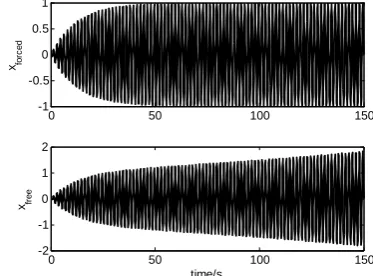
rad/s.

The initial oscillation curves are showed in Fig.1. After systemic implementation process of the method the instantaneous amplitude of processed free and forced oscillation are showed in Fig.2.

0 50 100 150 -1

-0.5 0 0.5 1

xfo

rc

e

d

0 50 100 150 -2

-1 0 1 2

time/s

xfr

e

[image:4.595.326.513.399.537.2]

e

Fig. 1 Oscillating curves of free oscillation and forced oscillation

120 125 130 135 140 145 150 0.8

1 1.2 1.4 1.6 1.8 2

time/s

A

m

pl

it

ude

[image:4.595.319.514.557.702.2]

Forced oscillation Weak damp oscillation

Fig. 2 Instantaneous amplitude of processed free and forced oscillation

(5)

free oscillation has directional changing trend, but the instantaneous amplitude of processed forced oscillation doesn’t have directional changing trend. So the oscillation types of oscillation in (24) and (25) can be identified exactly by the method proposed in this paper. So the method in this paper can overcome the shortcoming of the method in [13].

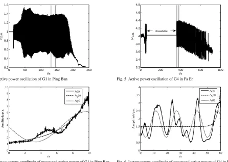
B. Actual incidents

Consider two practical oscillation incidents in China Southern Power Grid. Oscillation in Ping Ban and Fa Er is showed in Fig.3 and Fig.5 respectively. Data between two vertical lines in Fig.1 and Fig.3 is chosen as the input data. Employing the systemic implementation process in section

III, we get fitting coefficients and goodness, correlation coefficients and oscillation type identification results showed in Table I. The curves of instantaneous amplitude and its fitting results are showed in Fig.4 and Fig.6. In Ping Ban oscillation, SSE and RMSE under (20) are smaller than that under (21), and meanwhileCD and R under (20) are bigger than that under (21), therefor we consider the oscillation as

weak damping oscillation. In Fa Er oscillation, SSE and RMSE under (20) are bigger than that under (21), and meanwhile CD and R under (20) are smaller than that under (21), therefor we consider the oscillation as forced oscillation. In order to improve the identification accuracy, we choose data in different time ranges as input data and employ the systemic implementation process in section III. The identification results for every single data range are showed in Table II. And we conduct statistical analysis for the identification results. The oscillation type whose number is more than 50% of the total time range number for every oscillation incident is the type identified at last. Oscillation types identified by the proposed method are consistent with the post-fault offline analysis results [16]-[17]. In Fa Er plant oscillation, the initial period of wave is unavailable, so the method in [12]-[13] cannot be used to identify the oscillation type. But the method proposed in this paper identified the oscillation type accurately.

0 50 100 150 200 250 0.2

0.4 0.6 0.8 1 1.2 1.4 1.6

t/s

P

/p.

[image:5.595.76.523.296.614.2]

u.

Fig. 3 Active power oscillation of G1 in Ping Ban

0 2 4 6 8 10

0 1 2 3 4 5 6 7 8 9 10

t/s

A

m

p

litu

d

e

/p

.u

.

A(t) A_e(t) A_l(t)

Fig. 4 Instantaneous amplitude of processed active power of G1 in Ping Ban

0 200 400 600 800 3.2

3.4 3.6 3.8 4 4.2 4.4 4.6 4.8

t/s

P

/p.

u.

Unavailable

Fig. 5 Active power oscillation of G4 in Fa Er

0 10 20 30 40 50 60 0

0.5 1 1.5 2 2.5 3 3.5 4

t/s

A

am

p

lit

u

d

e

/p

.u

.

A(t) A_e(t) A

l(t)

Fig. 6 Instantaneous amplitude of processed active power of G4 in Fa Er

TABLEI

FITTING COEFFICIENTS AND GOODNESS,CORRELATION COEFFICIENTS AND OSCILLATION TYPE IDENTIFICATION RESULTS

Plant Expression a b c SSE RMSE CD R Oscillation Type Identified

Ping Ban

bt

ae c 0.3272 0.3136 0.991 153.4 0.3925 0.9602 0.9799

Weak damping Oscillation

sin

a btc -2.404 0.482 3.728 1119 1.06 0.7103 0.8428

Fa Er

bt

ae c -0.833 0.4064 1.66 3465 0.7602 0.1281 0.3652

Forced Oscillation

sin

(6)

TABLEII

OSCILLATION TYPE IDENTIFICATION RESULTS IN DIFFERENT TIME RANGES

Plant Start Time (s) End Time (s) Oscillation Type Identified Statistics Oscillation Type Identified at Last

Ping Ban

70 80 Weak damping Oscillation

88% WDO Weak damping Oscillation

80 90 Forced Oscillation

Fa Er

88% FOO Forced Oscillation

V. CONCLUSION

The instantaneous amplitude of weak damping oscillation has certain directional trend but that of forced oscillation does not have. We grasp and amplify this discriminative difference to identify oscillation types by a method based on EMD and HT. In this method, repeating EMD and square calculation alternately n times, the damp factor has been amplified by a factor of nth power of 2. And then here come two different results: directional changing trend of the amplitude of weak damping oscillation becomes more obviously but the amplitude in forced oscillation keeps constant or fluctuates around a constant not having any directional changing trend. We acquire the instantaneous amplitude of oscillation and use two different expressions to approximate it and analyze the correlation between the fitting results and it. Finally, we determine the oscillation types according to the goodness of fit and correlation coefficients. We use a simple test to illustrate the advantage of the method. The method is validated in actual oscillation incidents. The method utilizes WAMS data and has the potential for online application.

REFERENCES

[1] E. Grebe, J. Kabouris, S. Lopez Barba, and W. Sattinger et al., “Low frequency oscillations in the interconnected system of continental Europe”, IEEE PES GM, Minneapolis, 2010.

[2] F.P. Demello and C. Concordia, “Concepts of synchronous machine stability as affected by excitation control,” IEEE Trans. Power App. Syst., vol. PAS-88, no. 4, pp. 316–329, Apr. 1969.

[3] R. T. H. Alden and A. A. Shaltout, “Analysis of damping and synchronous torques: Part I—a general calculation method,” IEEE Trans. Power App. Syst., vol. PAS-98, no. 5, pp. 1696–1700, Sep./Oct. 1979.

[4] R. T. H. Alden and A. A. Shaltout, “Analysis of damping and synchronous torques: Part II—effect of operation conditions and

machine parameters,” IEEE Trans. Power App. Syst., vol. PAS-98, no. 5, pp.1701–1707, Sep. /Oct. 1979.

[5] M. A. Magdy, and F. Coowar, “Frequency domain analysis of power system forced oscillations,” Proc. Inst. Elect. Eng., Gen., Transm., Distrib, vo1.137, pp. 261-268, 1990.

[6] C. D. Vournas, N. Krassas, and B. C. Papadias, “Analysis of forced oscillations in a multi-machine power system,” in Proc. 4th Int. Conf. Control, 1991, pp. 443-448.

[7] N. Rostamkolai, R. J. Piwko, and A. S. Matusik, “Evaluation of the impact of a large cyclic load on the LILCO power system using time simulation and frequency domain techniques,” IEEE Trans. Power Syst., vol. 9, no. 3, pp. 1411-1416, 1994

[8] J. Ma, P. Zhang, and H. J. Fu, et al., “Application of phasor measurement unit on locating disturbance source for low-frequency oscillation,” IEEE Trans. Smart Grid, vol. 1, no. 3, pp. 340–346, Dec. 2010.

[9] L. Chen, Y. Min, and W. Hu, “An energy-based method for location of power system oscillation source,” IEEE Trans. Power Syst., vol. 28, no. 2, pp. 828–836, May. 2013.

[10] Y. Li, C. Shen and F. Liu, “An energy-based methodology for locating the source of forced oscillations in power systems,” in Proc. 8th Powercon, Auckland, New Zealand, Oct, 2012, pp. 1–6.

[11] Y. Li, C. Shen and F. Liu, “A methodology for power system oscillation analysis based on energy structure,” Automation of Electrical Power, vol. 37, no. 13, pp. 49–56, 2013, in Chinese. [12] Y. Li, W.S. Jia and W.F. Li, “Online identification of power oscillation

properties based on the initial period of wave,” Proc. CSEE, vol.33, no.25, pp.54-60, 2013, in Chinese．

[13] H. Ye, Y.B. Song and Y.T. Liu, “Forced power oscillation response analysis and oscillation type discrimination,” Proc. CSEE, vol.33, no.34, pp.197-204, 2013, in Chinese．

[14] N.E. Huang and S.S. Shen, Hilbert-Huang transform and its applications. Singapore: World Scientific Press, 2005.

[15] W.J. Conover, Practical nonparametric statistics. US: John Wiley & Sons, 1980.

[16] L. Chen, Y. Min and W. Hu, “Low frequency oscillation analysis and oscillation source location based on oscillation energy part two method for oscillation source location and case studies,” Automation of Electric Power, vol. 36, no. 4, pp. 1-5,27, 2012, in Chinese.