Abstract—The theory and methods for the Bayesian meta-analysis are motivators for this article. The methodology for hierarchical modeling for Bayesian meta-analysis is provided, along with detailed discussion of the theory. The impact of choosing different likelihood functions in Bayesian hierarchical modeling is discussed. A practical example of the meta-analysis for the oropharyngeal adverse events induced by inhaled corticosteroid is provided to illustrate the methods.
Index Terms— meta-analysis, Bayesian, Hierarchical Model, MCMC method, Binomial Likelihood
I. INTRODUCTION
HOUGH Bayesian modeling has been proposed as a
potential methodology for synthesizing all available evidence to inform decision making, few practical applications of Bayesian methods for combining data exist. Developing a potential application of these methods was the objective of this study, which sought to analyze a Bayesian meta-analysis using hierarchical modeling based on different Likelihood Functions (i.e. Different distributions). In addition, Bayesian meta-analysis was compared to traditional Peto odds ratio meta-analysis.
Oropharyngeal adverse events associated with inhaled corticosteroid (ICS) use was selected as the topic of this analysis because these adverse events can affect drug regimen adherence. Also, these effects have been studied less extensively than those that occur systemically and thus provides an open area of investigation.
This study will assess the risk of ICS-induced oral candidiasis among currently available therapies. A search in MEDLINE (January 1966 to June 2004) and EMBASE (January 1974 to June 2004) was conducted using indexed MedDRA terms for oropharyngeal adverse events. This yielded a total of 23 studies (containing 59 drug arms) that were evaluated for incidence of oral candidiasis. Odds ratios
Manuscript received June 16, 2014; revised August 8, 2014.
Hal Li, Manager, Principal Biostatistician, Biostatistics, is with the Accenture, Life Sciences, Berwyn, PA 19312, USA; Phone: 610-766-2297; e-mail: [email protected].
(ORs) were used to determine the rate of ICS-induced adverse events.
II. DATACOLLECTIONMETHOD
Oropharyngeal adverse events have been linked to a variety of causes. For example, oral candidiasis may be a result of reduced local immunity or an increase in salivary glucose levels, both of which encourage Candida albicans growth. Other factors that affect the rate of oral candidiasis include ICS dose, device, particle size, and percentage of ICS deposited in the oropharynx.
The objectives of this meta-analysis were to evaluate the degree of ICS-induced oral candidiasis among different ICSs.
A. Search Strategy
A computerized search in the MEDLINE (January 1966 to June 2004) and EMBASE (January 1974 to June 2004) databases was conducted using appropriately indexed MedDRA terms. These terms included the following: candidiasis, dysphonia, hoarseness, pharyngitis, thrush, throat irritation, voice alteration/ dysfunction, distorted voice, laryngeal/pharyngeal pain, oral fungal infection, cough, oropharyngeal/ esophageal adverse event, dose, local safety, incidence, prevalence, epidemiology, spacer, aerosol, asthma, and inhaled corticosteroids.
A. Search Criteria
Only randomized, placebo-controlled studies, with an emphasis on oral ICSs (single entity or combination therapy) for the treatment of persistent asthma of all severities, were eligible for inclusion (chronic obstructive pulmonary disease was excluded).
The included studies were efficacy and safety studies not specifically designed to report local safety. Study populations were limited to adults and adolescent cohorts only. Furthermore, only studies that reported appropriate information on patient demographics and study design were included. The 23 selected studies along with the treatment and end points of those studies are listed in Table 1:
The Impact of Choosing Different Likelihood
Functions in Bayesian Hierarchical Modeling
for Meta-Analysis: A Meta-analysis on
Oropharyngeal Adverse Events Induced by
Inhaled Corticosteroid
Hal Li
Table 1
Selected Oral ICS Studies
Study Design Treatment (dose & delivery
device) End points/outcomes Kavuru et al, 2000[1] DB, R, PC (12 wks)
SAL (50 µg) + FP (100 µg) bid DPI or SAL (50 µg bid DPI) or FP (100 µg bid DPI) or PBO
PFT and AS better w/SAL+FP vs all groups; AEs similar Shapiro et al, 2000[2] DB, R, PC (12 wks)
SAL+FP (50 and 250 µg bid DPI) or SAL (50 µg bid DPI) or FP (250 µg bid DPI) or PBO
PFT and AS better w/SAL+FP vs all groups Kemp et al, 1999 [3] DB, R, PC (12 wks)
BUD (200−400 µg bid DPI) or PBO
PFT and AS better w/BUD vs PBO; B and S cortisol NS Busse et al, 1998 [4] DB, R, PC (12 wks)
BUD (100−800 µg bid DPI) or PBO
PFT and AS better w/BUD vs PBO; AEs similar Pearlma
n et al, 1997[5]
DB, R, PC (12 wks)
FP (50−250 µg bid DPI) or PBO for
PFT and AS better w/FP vs PBO; AEs similar Nathan et al, 2000[6] DB, R, PC (12 wks)
FP (100−500 µg qd DPI) or PBO
PFT and AS better w/ FP vs PBO; AEs similar; S cortisol NS
Chervins ky et al, 1994[7]
DB, R, PC (8 wks)
FP (25−500 µg bid MDI) or PBO
PFT and AS better w/FP vs PBO; AEs were similar; S cortisol NS Condemi et al, 1997[8] DB, R, PC (24wks)
FP (250 µg bid DPI), TAA (200 µg q4 MDI/spacer) or PBO
PFT and AS better w/FP vs PBO or TAA; higher rates of OC w/FP; B cortisol NS Chervins
ky et al, 2002[9]
DB, R, PC (4 wks)
MF- CFC (56−500 µg bid MDI), BDP (168 µg bid MDI) or PBO
PFT and AS better w/MF and BDP vs PBO Corren et al, 2003 [10] DB, R, PC (8 wks)
MF (440 µg qd DPI/spacer), BDP (400 µg qd DPI/ spacer) or PBO
PFT and AS better w/MF vs BUD or PBO; AEs similar Fish et al, 2000 [11] DB, R, PC (12 wks)
MF (400−800 µg bid DPI) or PBO
OCS dose significantly reduced w/MF vs PBO; PFT better w/MF Laviolett
e et al, 1999 [12]
DB, R, PC (16 wks)
MON (10 mg qd) and BDP (200 µg bid MDI), BDP (200 µg bid MDI), MON (10 mg qd) or PBO
PFT and AS better w/MON plus BDP; AEs similar Gross et al, 1999 [13] SB, R, PC (12 wks)
BDP-HFA (200 µg bid MDI), BDP-CFC (400 µg bid MDI) or PBO
PFT and AS better w/BDP vs PBO; AEs similar Nelson et al, 1999 [14] DB, R, PC (16 wks)
FP (500−1000 µg bid DPI) or PBO
OCS dose significant reduced w/FP vs PBO; PFT better w/FP Welch et al, 1999 [15] DB, R, PC (8 wks)
TAA-HFA (150−600 µg qd MDI/ spacer), TAA-CFC (150−600 µg qd MDI/spacer) or PBO
PFT and AS better w/TAA vs PBO; AEs similar Nathan et al, 1997 [16] DB, R, PC (28 days)
BDP (84 µg bid [2 inhalations], 42 µg bid [4 inhalations], 84 µg bid [8 inhalations] MDI) or PBO
PFT and AS better w/BDP vs PBO; AEs similar Boe et al, 1989 [17] DB, R, PC (≥22 wks)
BDP (200−500 µg bid MDI), BUD (200−400 µg bid MDI) or PBO for
PFT and AS similar between groups and better vs PBO; higher rates of OC w/BUD vs BDP
Study Design Treatment (dose & delivery
device) End points/outcomes Bronsky et al, 1998 [18] DB, R, PC (8 wks)
BDP (336 µg qd MDI), TAA (800 µg qd MDI/spacer) or PBO
PFT and AS similar between active groups; AEs similar Galant et al, 1999 [19] DB, R, PC (12 wks)
FP (500 µg bid DPI), FP (500 µg bid MDI) or PBO
PFT and AS similar between groups and better vs PBO; AEs similar Nayak et al, 2000 [20] DB, R, PC (12 wks)
MF (200−400 µg qd DPI) or PBO
PFT and AS better w/MF vs PBO; AEs similar Bernstei
n et al, 1999 [21]
DB, R, PC
(12 wks)
MF (100−400 µg bid DPI), BDP (168 µg bid MDI) or PBO
PFT and AS better w/ MF and BDP vs PBO Wolfe et al, 1996 [22] DB, R, PC (12 wks)
FP (100−500 µg bid MDI) or PBO
PFT and AS better w/FP vs PBO; AEs higher w/FP vs PBO Metzger et al, 2002 [23] DB, R, PC (12 wks)
BUD (400 µg qd DPI) or PBO
PFT and AS better w/BUD vs PBO; AEs similar BUD=budesonide;BDP=beclomethasone dipropionate;FP=fluticasone propionate; MF=mometasone furoate; MON=montelukast; SAL=salmeterol; TAA=triamcinolone acetonide; PBO=placebo; DPI=dry powder inhaler; MDI=metered dose inhaler; qd=once daily; bid=twice daily; AEs=adverse events; OC=oral candidiasis; OCS=oral corticosteroids; FEV1=forced expiratory volume in 1 second; DB=double blind; SB=single blind; R=randomized; PC=placebo controlled; PFT=pulmonary function tests; AS=asthma symptoms; B=basal; S=stimulated; NS=no significant suppression
III. Bayesian Hierarchical Modeling for Meta-Analysis
Meta-analysis is an important technique that combines information from different studies. When there is no prior information for thinking any particular study is different from another, Bayesian meta-analysis can be treated as a hierarchical model. This assumption, known as exchangeability, then allows for a Bayesian random-effects model, which assumes that there is no such prior information and therefore treats all studies equally.
A. Bayesian Hierarchical Modeling Use Normal Approximation to the Likelihood
Normal approximation to binomial likelihood is a classical method that is commonly used in meta-analysis.
Assume that there were total N_trtj and N_ctrlj patients in the jth study. Assume also that the number of oral candidiasis observed in the jth study active treatment arm and control treatment arm as event_trtj and event_trtj respectively. Given, these assumptions, let Yj be the odds ratio of oral candidiasis for the jth study:
[1]
It is possible to estimate the treatment effect θj, j=1,…,n, through the means of an approximate normal distribution,
where θj is the study-specific effect and sj2 is the known variance of log(Yj). For sj2, If all studies have large sample sizes (more than 30 persons in each group in nearly all of the studies), it is possible to use the approximate sampling variance of θj:
[2]
If the odds ratios are exchangeable between the studies, then the treatment effect in each trial can be considered to be a random quantity drawn from some population distribution. In a Bayesian framework, this means that it is possible to place a common prior distribution on the exchangeable random-effects parameters θj:j=1,…,n.
θj ~ normal(μ, τ2)
where μ is the population average of the treatment effect across all studies and τ2 is the between-study variation. In this meta analysis, the following non informative priors are placed on the hyper parameters μ, and τ2:
μ ~ normal(0, 32)
τ2 ~ igamma(shape = 0.01, scale = 0.01)
B. Bayesian Hierarchical Modeling Use Binomial Likelihood
Emulating the binomial model as outlined in Spiegelhalter, Abrams, and Myles (2004) [3], one can use the following model, where the treatment and control groups have their own binomial likelihood functions, with oral candidiasis probabilities pj and qj in the treatment group and control group respectively:
event_trtj ~ binomial(N_trtj, pj) event_ctrlj ~ binomial(N_ctrlj , qj)
Let the log odds for the control group be ϕj and let the log odds for the treatment group be θj + ϕj as follows:
ϕj = log(qj/(1- qj ))
θj = log(pj/(1- pj ))
Then θj is the log odds ratio:
If treatment group risks are exchangeable, then it can be assumed that θj:j=1,…,n, are random-effects parameters that are drawn from some common prior distribution:
π(θj) = normal(μθ, σ2θ)
If the control group risks are also exchangeable, then one can consider ϕj: j=1,…,n, as other random-effects parameters with the following common prior:
π(ϕj) = normal(μϕ, σ2ϕ)
In this meta-analysis the following noninformative priors are placed on the hyperparameters μ, and σ2:
π(μθ) and π(μϕ) ~ uniform(-1.5, 1.5)
π(σθ2) and π(σϕ2) ~ uniform(0, 8).
IV. BAYESIAN ANALYSIS AND MCMCESTIMATION
METHOD
Bayesian analysis is a statistical method that makes inferences on unknown quantities of interest by combining prior beliefs about the quantities of interest and information contained in an observed set of data. Supposing that the analysis is interested in estimating θ from a data set: X={x1 ,…,xn}. Bayes theorem provides a solution by using a
well known rule about conditional probabilities:
Overall, Bayesian inference is based on the posterior distribution of the parameter P(θ|X). However, in order to derive the posterior distribution, the prior distribution must already be specified, P(θ) – the distribution of θ. The likelihood function P(X|θ) must also be determined from the data observed. From (1), it is apparent that the P(θ|X) is proportional to (i.e. has the same shape as) the product of the likelihood function and the prior distribution of the data:
P(θ|X)~P(X|θ)P(θ)
Having derived the posterior distribution, P(θ|X), in Bayesian analysis all further inferences about θ will be derived from that distribution.
In theory, Bayesian methods are straightforward—the posterior distribution contains everything needed to carry out inference. In practice, the posterior distribution can be difficult to estimate precisely. One popular and very general simulation method is a Markov chain Monte Carlo (MCMC). MCMC methods, sample successively from a target distribution, with each sample depending on the previous one, hence the notion of the Markov chain. Monte Carlo integration computes an expectation by averaging the Markov chain samples
where g(.) is a function of interest and θt are samples from
p(θ) on its support S.
The SAS proc MCMC procedure was applied for this meta analysis. The MCMC procedure uses a special case of the MCMC method, the random walk Metropolis algorithm (Metropolis et al. 1953; Hastings 1970) [1], [2] to generate a sequence of draws from the joint posterior distribution of the parameters. This procedure is capable of constructing an
j
j j
i i i
i
P
X
P
P
X
P
X
P
X
P
X
P
)
(
)
|
(
)
(
)
|
(
)
(
)
,
(
)
|
(
optimal proposal distribution in the random walk Metropolis algorithm, and the procedure can be used to generate samples from an arbitrary density. Once samples are obtained, one can carry out additional statistical inference as desired.
V. META ANALYSIS USING PETO METHOD –A
FREQUENTIST’S APPROACH BAYESIAN ANALYSIS AND
MCMCESTIMATION METHOD
As a comparison, Peto’s method (Yusuf S, Peto R, Lewis J, Collins R, Sleight P et al. 1985
[4]
) was applied to estimate the pooled odds ratio. Peto and colleagues presented a method for pooling odds ratios. This method is not mathematically equal to the classical odds ratio, but it has come to be known as the ’Peto odds ratio’. The Peto odds ratio can cause bias, especially when there is a substantial difference between the treatment and control group sizes, but it performs well in many situations.Assuming that we want to estimate:
1
...
r
.Under a broad assumption one can derive:
)
,
(
~
i ii
i
w
N
w
w
.Then it is possible to estimate θ by
i i i
w
w
. with 95%CI
i
w
1
96
.
1
.In order to test for the heterogeneity among the studies, the following Q statistics will be used:
i r
i
i
w
Q
1
2
)
(
21
~
rVI. RESULTS
A. Bayesian Hierarchical Model Using Binomial Likelihood
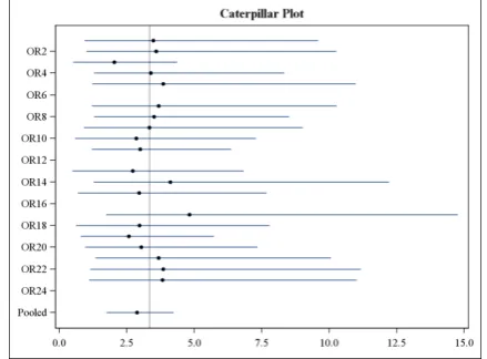
[image:4.595.314.537.95.262.2]The pooled estimate of the odds ratio of oral candidiasis was 2.54, indicating that oral candidiasis was more likely in inhaled corticosteroid (ICS) treatment compared to in the placebo. However the HPD credible interval estimates show the 95% credible interval is (0.95, 4.56). Since this interval includes 1, the oral candidiasis was not statistically significantly worse in the ICS treatment compared to that in the placebo. There was some variation among the treatment effects.
Figure 1 shows the posterior means and the 95% equal-tail credible intervals of odds ratios from the 23 studies and for the pooled odds ratio. It looks like the ICS treatment caused the most oral candidiasis in Study 11 and least oral candidiasis in Study 4. Because there were many studies that observed 0 oral candidiasis in the placebo arms, The Yj and sj2 can not be calculated by using the formula [1] and [2]. As the result, the odds ratio and its 95% credible
intervals cannot be estimated, and the pooled odds ratio was based only on the data from the 8 studies, for which Yj and sj2 can be calculated.
Figure 1: Odds Ratio and its 95% Credible Intervals based on Bayesian Hierarchical Model Using Normal Approximation to the Likelihood
B. Bayesian Hierarchical Model Using Binomial Likelihood
[image:4.595.46.291.300.444.2]The pooled estimate of the odds ratio of oral candidiasis was 2.88, indicating that oral candidiasis was more likely in an inhaled corticosteroid (ICS) treatment compared to that in the placebo. In addition, the HPD credible interval estimates show the 95% credible interval was (1.79, 4.25). Since this interval does not include 1, the oral candidiasis was statistically significantly worse in the ICS treatment compared to that in the placebo. The variation among the treatment effects was not significant.
Figure 2 shows the posterior means and the 95% equal-tail credible intervals of odds ratios from the 23 studies and for the pooled odds ratio. Because the exact method was used, for all the studies, except four of them (Study 2, 6, 12, and 16), odds ratio and its 95% credible intervals can be estimated.
Figure 2: Odds Ratio and its 95% Credible Intervals based on Bayesian Hierarchical Model Using Binomial Likelihood
[image:4.595.316.536.545.707.2]As a comparison, Peto’s method was applied to estimate the pooled odds ratio. The pooled estimate of the odds ratio of oral candidiasis was 2.87, indicating that oral candidiasis was more likely in an inhaled corticosteroid (ICS) treatment compared to that in the placebo. The 95% confidence interval (CI) was (2.01, 4.10). Since this interval does not include 1, the oral candidiasis was statistically significantly worse in the ICS treatment compared to that in the placebo. The p-value from the z statistics was <0.0001, This confirms the same conclusion from the 95% CI. The Q statistic was 7.26 (p=0.999), this means there was no evidence of heterogeneity among studies.
VII. DISCUSSION
The standard normal approximation method might not be appropriate because the approximation becomes less precise in extreme probabilities. For example, in the multi-studies dataset, the oral candidiasis rates were 0 for many placebo and treatment groups. The odds ratio and its 95% credible intervals cannot be estimated in these cases, and therefore the pooled odds ratio was based only on the data from 8 studies. Therefore, an alternative approach is to use the exact binomial likelihood approach as opposed the normal approximation.
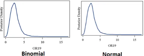
As a comparison, the kernel densities of the odds ratios for the Study 19 are calculated by using the approximate normal likelihood and the exact binomial likelihood functions. Figure 3 compares the kernel density plots of the odds ratios that are produced by using these two likelihood functions for the Study 19. For this study, where the normal likelihood can be applied, the kernel density plots that are produced by using the approximate normal likelihood and the exact binomial likelihood are very similar.
[image:5.595.49.292.569.664.2]In contrast, there are a huge number of studies for which the odds ratio cannot be estimated by the normal method. As described earlier, the pooled odds ratio was based only on the data from the 8 studies for which Yj and sj2 can be calculated, whereas the exact binomial’s estimate were based on 19 studies. Thus, there was a huge difference in the pooled odds ratio estimated from these two methods.
Figure 3: Kernel Density Plots for Study 19
The estimate on the pooled odds ratio from the exact binomial Bayesian method and the frequentist’s Peto’s method are very similar. The 95% credible interval and the 95% confidence interval are similar and consistent. The assumption exchangeability for the Bayesian method was confirmed by the Q heterogeneity statistics 7.26 (p=0.999) from Peto’s method.
VIII. CONCLUSION
Results from this meta-analysis suggest that before performing meta-analysis by a Bayesian method, one should perform some data checks by the traditional frequentist method. Assessing the exchangeability of the Bayesian method by the Q heterogeneity statistics from the Peto’s method is an important factor that needs to be assessed. This will make sure the Bayesian analysis starts from a proper beginning. When we decide which likelihood distribution is to be selected, caterpillar plots for the odds ratio and its 95% credible intervals need to be created. From these plots, one can examine if any “extreme probability” exist. This assessment will be helpful to decide which likelihood distribution to be used for the Bayesian meta-analysis.
Results from this meta-analysis confirm observations that ICS use is associated with a significant risk of oropharyngeal adverse events (oral candidiasis) compared with placebo. Notably, these adverse events can trigger clinical discomfort and may affect adherence to treatment and quality of life in patients. However, ICSs may be the most effective controller medication available for some diseases and potential adverse events are generally outweighed by the benefits of treatment.
As such, methods to reduce ICS-related oropharyngeal adverse events (ie, mouth washing or use of a spacer) or the use of ICSs with improved safety profiles should be the primary tool to minimize the impact of adverse effects, while still providing patients with the most effective treatment.
REFERENCES
[1] Hastings, W. K. (1970), “Monte Carlo Sampling Methods Using Markov Chains and Their Applications,” Biometrika, 57, 97–109. [2] Metropolis, N., Rosenbluth, A. W., Rosenbluth, M. N., Teller, A. H.,
and Teller, E. (1953), “Equation of State Calculations by Fast Computing Machines,” Journal of Chemical Physics, 21, 1087–1092. [3] Spiegelhalter, D. J., Abrams, K. R., and Myles, J. P. (2004),
“Bayesian Approaches to Clinical Trials and Health-Care Evaluation,” Chichester, England: John Wiley & Sons.