Abstract---This paper proposes a technique to design the (n-2) stage PD (Proportional-Derivative) controller cascaded with the PID (Proportional-Integral-Derivative) controller in accordance with nth order plants. The Continuous-Time (CT) design is firstly reviewed to show the advantages of the Kitti’s method. The proposed technique is based on the Kitti’s method in combination with the use of First Order Hold (FOH) to discretize the CT plant and Delayed First Order Hold (DFOH) to discretize the CT controller for obtaining the proper Discrete-Time (DT) controller structure. The simulation results confirm that the proposed design technique can be applied to the DT framework with better specifications than it was expected.
Index Terms— Continuous-Time / Discrete-Time PID×(n-2) PD controllers, First Order Hold, Delayed First Order Hold
I. INTRODUCTION
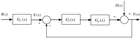
t is known that most industrial plants are type 0 and consist of three to five first order lags or dead time plus one first order lag [1]. However, the PID controller is properly applied to a typical second order plant only. In order to control a third order system to obtain the given specifications, an analytic PIDA (Proportional-Integral-Derivative-Acceleration) controller design technique is then proposed [2]. For a third or higher nth order plant, a design method based on root locus technique for the PID×(n-2) stage PD cascade controllers in CT framework has been presented [3]. This design technique is aimed to satisfy the desired specifications without trial and error. Then, the forward controller is employed to decrease the overshoot, and the controlled system structure becomes two degree of freedom (2-DOF) control system as shown in Fig. 1.
Manuscript received December 19, 2016; revised January 9, 2017. C. Chiengtee is with Department of Instrumentation and Control Engineering, Faculty of Engineering, King Mongkut’s Institute of Technology Ladkrabang, Bangkok, Thailand, 10520 (e-mail: [email protected]).
P. Pannil is with Department of Instrumentation and Control Engineering, Faculty of Engineering, King Mongkut’s Institute of Technology Ladkrabang, Bangkok, Thailand, 10520, (phone : 662-329-8348; fax: 662-329-8349; e-mail: [email protected]).
P. Ukakimaparn is with Department of Instrumentation and Control Engineering, Faculty of Engineering, King Mongkut’s Institute of Technology Ladkrabang, Bangkok, Thailand, 10520 (e-mail: [email protected]).
T. Trisuwannawat is with Department of Instrumentation and Control Engineering, Faculty of Engineering, King Mongkut’s Institute of Technology Ladkrabang, Bangkok, Thailand, 10520 (e-mail: [email protected]).
( )
f
G s
( )
X s
( )
P
G s ( )
c
G s
( )
R s
( )
D s
( )
Y s
+ −
[image:1.595.309.546.217.282.2]+ +
Fig. 1. Structure of the 2-DOF control system.
For DT framework, three generations of these PID×(n-2) stage PD cascade controllers have been proposed recently. The first design for the DT PID×(n-2) stage PD cascade controllers is using Zero Order Hold (ZOH) discretization method [4], while the second one is using “Tustin” or bilinear discretization method to design the controllers in z-plane [5]. The third concept to design DT controllers is also using “Tustin”, but it is required to transform the CT designed controller from s-plane to z-plane [6]. In order to be an alternative method for DT controller designs, this paper presents an effective design technique using FOH and DFOH discretizations as well as using Kitti’s method. The MATLAB simulation results for verifying the controller performances are also included.
II.METHODOLOGY
[image:1.595.312.546.572.695.2]Fig. 2 shows the steps for design of digital control systems [7], which are 2 major steps; plant modeling and controller design.
Fig. 2. Steps of the digital control system design.
A. Problem Statement
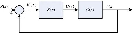
From a block diagram of Fig. 3, we need to find the PID×(n-2) stage PD cascade controllers K(s) or K(z) for the plant G(s), so that the given desired specifications could be acceptably achieved.
Discrete-Time PID×(n-2) Stage PD Cascade
Controllers with First Order Hold and
Delayed First Order Hold Discretizations
Channarong Chiengtee, Pittaya Pannil, Prapart Ukakimaparn, and Thanit Trisuwannawat
( ) R s
( )
K s U s( ) G s( ) Y s( )
− +
( ) R s
( )
K s U s( ) G s( ) Y s( )
− +
) ( s
[image:2.595.56.282.50.107.2]E
Fig. 3. Block diagram of typical control system.
B. Continuous–Time Framework
Let the nth order plant G(s) be controlled by the cascade controllers K(s), their transfer function is assumed to be
1 2
( ) ,
( 1)( 1) ( 1)
1
; 3, 0.
( 1)( 3)( 6) n N
p K
G s
s T s T s T s
n N
s s s
=
+ + +
= = =
+ + +
⋯
(1)
The transfer function of the PID controller can be stated as
1 2
( )( )
( ) i ,
PID p d pid
K s z s z
K s K K s K
s s
+ +
= + = (2)
where Kp is a proportional gain, Ki is an integral gain, and Kd is a derivative gain. Hence, the PD controller transfer function is
( ) ( ).
PD p d pd pd
K s =K +K s=K s+z (3)
The open-loop transfer function for the PID×(n-2) stage PD cascade controllers K(s) and the plant G(s) can be given by
1 2
1 2
( 2) PD
PID Controller
( )( ) ( )
( ) ,
( )( ) ( )
th order Plant
( 3.1)( 6.1)( )
.
( 1)( 3)( 6)
pid pd pd n
N
p
pd
n
K s z s z K s z K
KG s
s s s p s p s p
n
s s s z
K
s s s s
−
+ + × +
=
⋅ + + +
+ + +
=
⋅ + + +
⋯
⋯
(4)
By using Kitti’s method, z1 = 3.1 and z2 = 6.1 are firstly
assigned, then find only zpd and K from the root locus angle and magnitude conditions as follows.
( ) (2 1) , 0,1, 2, ,
( ) 1.
KG s k k
KG s
π = ± + =
=
∡ ⋯
(5)
The desired specifications to be designed are usually specified in terms of transient and steady state response characteristics of the control system to a unit-step input, exhibited by a pair of complex-conjugate dominant
closed-loop poles 1 2
d n n
s ±= −ζω ±jω −ζ as follows:
(
)
2
1
2
Percent Overshoot ( . .) 100% 5%, ln 0.02 1
Settling Time ( ) 2secs.
( 2%) s
n P O e
t
ζπ ζ
ζ ζω
−
−
= × =
− −
= =
±
(6)
From the given desired specification in term of the Percent Overshoot (P.O.), the damping ratio is
2 2
2
. . . .
ln ln 0.69.
100 100
P O P O
ζ = π + =
(7)
From the given Settling Time {ts(±2%)}, the undamped natural frequency is
(
2)
ln 0.02 1
3.069 rad./sec.
n
s
t
ζ
ω
ζ
− −
= = (8)
Hence, one of the dominant closed-loop poles is located at 2.118 2.221.
d
s = − + j (9)
The open-loop transfer function without zpd at sd is
66.139 29.147
( 3.1) ( 6.1)
( ) ,
( 1) ( 3) ( 6)
133.639 116.715 68.333 29.771
0.069 0.13 0.411 106.829 .
d d
d
d d d d
s s
KGwozpd s
s s s s
j
+ +
=
+ + +
= − + =
∡
(10)
The angle from the zero zpd to sd is
(
)
arg[zpd]= −π arg KGwozpd s( d) =73.171 . (11)
The location of the zero zpd can find from
(
)
Im( )
Re( ) 2.789.
tan arg[ ] d
pd d
pd s
z s
z
= + = (12)
Now, it is implied that
95.286 73.171
( 3.1)( 6.1) ( 2.789)
( ) 180 .
( 1)( 3)( 6)
348.457
d d d
d
d d d d
s s s
KG s
s s s s
+ + +
= = −
+ + +
∡ ∡ (13)
The open-loop gain K can be found from the magnitude condition of the root locus technique as follows:
2.39 4.473 3.069 2.486
1 3 6
3.174.
3.1 6.1 2.789
2.428 4.56 2.32
d d d d
d d d
s s s s
K
s s s
+ + +
= =
+ + + (14)
To decrease the overshoot caused by adding the zero (s+zpd) to the open-loop transfer function KG(s), the forward controller can be stated as
( ) pd .
f
pd z K s
s z =
-8 -6 -4 -2 0 -3
-2 -1 0 1 2 3
Real Axis
Im
ag
A
xi
s
[image:3.595.53.282.61.274.2] [image:3.595.53.283.100.417.2]sd
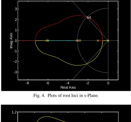
Fig. 4. Plots of root loci in s-Plane.
0 0.5 1 1.5 2 2.5 3
0 0.2 0.4 0.6 0.8 1 1.2
Time (secs)
A
m
p
lit
u
d
e
Fig. 5. Unit step responses.
The overall system is then approximated as if it is a standard second order system as follows:
2
2
( )
( )
,
( ) ( 1) ( )
8.854
.
2 0.701 2.976 8.854
pd pd
pd pd
n n
z K s z
Y s
R s s z s s K s z
s s
ζ ω ω
+
=
+ + + +
=
+ ⋅ ⋅ +
[image:3.595.265.545.103.578.2](16)
Fig. 4 shows the plots of root loci in s-Plane. The unit step responses with and without the forward controller are shown in Fig. 5, respectively.
C. Discrete-Time Framework
[image:3.595.49.217.477.555.2]To design the DT controller, the CT plant (or CT system) and CT controller can be discretized by FOH [9] and by DFOH [10], respectively. Then we design the DT controller in the same way as the CT framework.
Fig. 6. Discretization.
The DT transfer function of the CT plant G s with the ( ) sampling time T(sec/samples)is discretized by FOH is as follows:
2 2
( 1) 1
( ) z ( ) .
G z G s
Tz s
−
=
Z (17)
Hence, from (1) yields
2 2
( )
( 1) 1
( ) ,
( 1)( 3)( 6)
F s z
G z
Tz s s s s
−
=
⋅ + + +
Z (18)
where
2
2
( ) ,
( 1) ( 3) ( 6)
1 27 1 1 1
18 324 10 54 540
( ) .
( 1) ( 3) ( 6)
a b c d e
F s
s s s s
s
F s
s s s s
s
≡ + + + +
+ + +
−
−
= + + + +
+ + +
(19)
Then,
{
}
23
6
1 27
( )
18 ( 1) 324 ( 1)
1 1
10 ( ) 54 ( )
1
.
540 ( )
T T
T
Tz z
F s
z z
z z
z e z e
z
z e
− −
−
= +− − −
+ +
− − −
+ −
Z
(20)
Finally, we have
2
2 2
3 6
1 27 1 1 ( 1)
( )
18 324 10 ( )
1 ( 1) 1 ( 1)
.
54 ( ) 540 ( )
T
T T
z z
G z
T T z e
z z
T z e T z e
−
− −
= + − − + −
−
− −
+ +
− − −
(21)
For T =1/ 50 sec/samples,we obtain
3 2
3 2 1 0
3 6
7 3
6 3 2
6 6 1
7 0
( ) ,
( )( )( )
3.203 10 ,
0.98, 3.386 10 ,
, 0.942,
3.254 10 ,
0.887. 2.841 10 ,
T T T
T
T
T
z z z
G z
z e z e z e
e e e
β β β β
β β β β
− − −
− − −
− −
− −
+ + +
=
− − −
= ×
=
= ×
=
= ×
=
= ×
(22)
Then,
5 ( 9.5139)( 0.9608)( 0.970)
( ) 10 .
( 0.9802)( 0.9418)( 0.8869)
z z z
G z
z z z
− + + +
=
− − − (23)
[image:3.595.59.280.700.770.2]DFOH [10] is applied. Based on the DFOH, the desired DT transfer function can be stated as
(
1 2)
12
( )
( ) 1 2 K s .
K z z z
Ts
− − −
= − +
Z L (24)
Here,
(
)
(
3 2)
3 2 1 0
( ) ,
.
i
p d p d
K
K s K K s K K s
s
b s b s b s b s
= + + + = + + + (25) Then, 3 2
3 2 1 0
2 2
1 3 2
2 2 0 1 2 3 2 3 2 2 2 0 1 2 3
( ) 1
, ( )
1
( 1) ,
( 1) 2( 1)
( 1) ( )
1 ( 1)
( 1) 2( 1)
b s b s b s b K s
s
Ts Ts
b b
K s z
T T z
Ts
b
b Tz T z z
T z T z
b b
z z
K z
T T z
z
b
b Tz T z z
T z T z
− + + + = = + − + + + − − − = + − + + + − − ⋯ ⋯ L . (26)
Finally, we have
3 2
3 2 1 0
2 3 3 2 2 2 2 1 1 0 0 2 ( ) , ( 1)
2 2 0 0
6 4 2
1
,
6 2 2
2
2 0 0 0
( )( )( )
( ) .
( 1)
a b c
z z z
K z z z b b T T b T T T b
z z z z z z
K z K
z z
β β β β
β β β β + + + = − − − = − − − − − ≡ − (27)
From (22) and (26), the open-loop transfer function used to design the DT PID×(n-2) stage PD cascade controllers can be written as
2
5
( )( )( )
( ) ( )
( 1)
( 9.5139)( 0.9608)( 0.970)
10 .
( 0.9802)( 0.9418)( 0.8869)
a b c
z z z z z z
K z G z K
z z
z z z
z z z
− − − − = − + + + × − − − ⋯ (28)
By using Kitti’s Method to design the cascade controllersK z , let ( ) za =0.9518 and zb =0.8969. Then, the open-loop transfer function without (z−zc) is
2
5
( 0.9518)( 0.8969) ( )
( 1)
( 9.5139)( 0.9608)( 0.970)
10 .
( 0.9802)( 0.9418)( 0.8869) c
z z
KGwoz z K
z z
z z z
z z z
− − − = − + + + × − − − ⋯ (29)
The desired specifications for design of the controller K(z) are given in (6). Then the dominant closed-loop pole in z-Plane is
0.958 0.043,
1 50 sec/ sample.
d
T s d
z e j
T ⋅ = = + = (30)
Then, the necessary angle of the open-loop transfer function without the zero (z−zc) at the dominant closed-loop pole zd is
[
]
( ) 0.036 0.057,
arg ( ) 122.438 .
c d
c d
KGwoz z j
KGwoz z = − + = (31)
From the angle condition of the root locus method, the angle from zc to zd can be written as
[ ]
[
]
arg zc = −π arg KGwoz zc( d) =57.562 . (32)
Since, the angle of the zero (z−zc) is less than 90 , then zc is located at the left hand side of zd as follows.
[ ]
(
)
Im( )
Re( ) 0.931.
tan arg d c d c z z z z
= − = (33)
Another required parameter is the controller gain K, which can be found from the magnitude condition of the root locus method as follows.
1 ( d) ( d) 292.683.
K = K z G z = (34)
Finally, the controller transfer function can be stated by
2
2
( )( )( )
( ) ,
( 1)
( 0.9518)( 0.8969)( 0.931)
292.683 .
( 1)
a b c
z z z z z z
K z K
z z
z z z
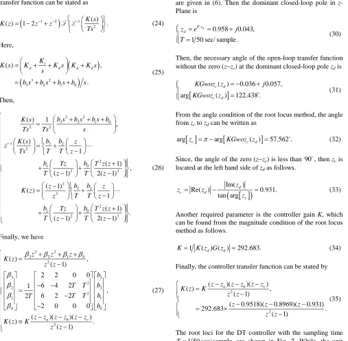
z z − − − = − − − − = × − (35)
The root loci for the DT controller with the sampling time 1 50 sec/ sample
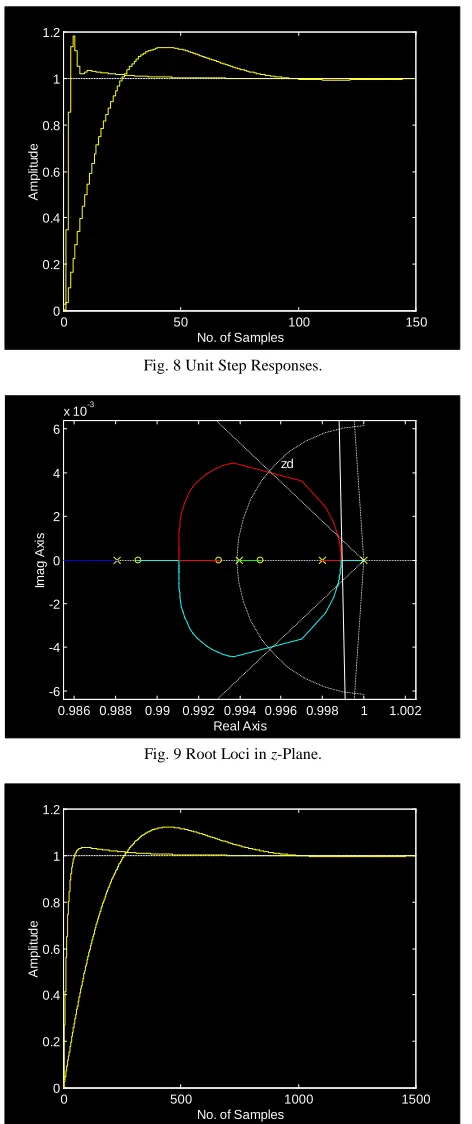
T = are shown in Fig. 7. While, the unit step response are shown in Fig. 8, respectively.
[image:4.595.49.556.65.562.2] [image:4.595.306.534.594.764.2]0.86 0.88 0.9 0.92 0.94 0.96 0.98 1 1.02 -0.06 -0.04 -0.02 0 0.02 0.04 0.06 Real Axis Im a g A xi s zd
0 50 100 150 0
0.2 0.4 0.6 0.8 1 1.2
No. of Samples
A
m
p
lit
u
d
[image:5.595.52.288.47.609.2]e
Fig. 8 Unit Step Responses.
0.986 0.988 0.99 0.992 0.994 0.996 0.998 1 1.002 -6
-4 -2 0 2 4 6
x 10-3
Real Axis
Im
a
g
A
xi
s
zd
Fig. 9 Root Loci in z-Plane.
0 500 1000 1500
0 0.2 0.4 0.6 0.8 1 1.2
No. of Samples
A
m
p
lit
u
d
e
Fig. 10 Unit Step Responses.
For the sampling time T = 1/500 sec/samples, the corresponding root loci and unit step responses are shown in Fig. 9 and Fig. 10, respectively. Where, the plant transfer function, the controller transfer function and the dominant closed loop pole are as follows:
8
2 3
10 ( 9.8595)( 0.9960)( 0.1006)
( ) ,
( 0.9980)( 0.9940)( 0.9881) 27660( 0.9950)( 0.9891)( 0.993)
( ) ,
( 1) 0.996 4.423 10 . d
z z z
G z
z z z
z z z
K z
z z
z j
−
−
= + + +
− − −
= − − −
−
= + ×
(36)
III. CONCLUSION
The design of PID×(n-2) stage PD cascade controllers in CT framework has been described to point out the aim of Kitti’s method, which provides that all desired specifications to be designed can be achieved without trial and error steps in the design process. However, the original design based on Kitti’s method uses the forward controller for decreasing undesired overshoot. Nowadays, the forward controller is rarely or never used, because there is alternate way to decrease the maximum percent overshoot by increasing the controller gain to be greater than the designed value, so that the plots of root loci are always toward the real axis along circular shape. If the sampling time is enough, all desired specifications are easily obtained.
REFERENCES
[1] David W. Pessen, “A New Look at PID Controller Tuning”, Transactions of the ASME, Journal of Dynamic Systems, Measurement, and Control, Vol. 116, pp. 553-557, Sept. 1994. [2] Seul Jung and Richard C. Dorf, “Analytic PIDA Controller Design
Technique for a Third Order System,” Proceedings of the 35th Conference on Decision and Control, pp. 2513-2518, Kobe, Japan, December, 1996.
[3] Thanit Trisuwannawat, Kitti Tirasesth, Jongkol Ngamwiwit and Michihiko Iida, “PID (n-2) stage PD cascade controller for SISO systems,” SICE’98 Proceedings of the 37th SICE Annual Conference, International session Papers, pp. 965-968, 1998. [4] Pittaya Pannil, Suksiri Kanchanasomranvong, Prapart
Ukakimaparn, Thanit Trisuwannawat, and Kitti Tirasesth, “Discrete PID×(n-2) stage Cascade Controller for SISO Systems,” SICE Annual Con- ference, pp. 1784-1787, The University Electro- Communications, Japan, August 20-22, 2008.
[5] Krit Smerpitak, Prapart Ukakimaparn, Thanit Trisuwannawat, and Prera Lavanprakai, “Bilinear Discrete PID×(n-2) stage PD Cascade Controller for SISO Systems,” 2012 12th International Conference on Control, Automation and Systems, pp. 1591-1596, in ICC (International Convention Center), Jeju Island, Korea, Oct. 17-21, 2012.
[6] Suralak Charoonsote, Prapart Ukakimaparn, Pittaya Pannil, and Thanit Trisuwannawat, “Discrete PID×(n-2) Stage PD Cascade Controllers Proposed by Kitti,” Proceedings of the 4th IIAE International Conference on Industrial Application Engineering, pp. 258-262, B-Con Plaza, Beppu, Japan, March 26-30,2016. [7] Hiroshi Fujimoto, "General Framework of Multirate Sampling
Control and Applications to Motion Control Systems", Ph.D. Dissertation, The University of Tokyo, submitted in December 2000 and published in March 2001.
[8] Ryozo Nagamune, MECH468/550P: Modern Control Engineering / Foundations in Control Engineering, Lecture Note # 6, Department of Mechanical Engineering, University of British of Columbia (UBC), Canada, 2008/2009.
[9] Jesse B. Hoagg, Seth L. Lacy, R. Scott Erwin, and Dennis S. Bernstein, “First-Order-Hold Sampling of Positive Real Systems And Subspace Identification of Positive Real Models,” Proceeding of the 2004 American Control Conference, pp. 861-866, Boston, Massachusetts, June 30 - July 2, 2004.