High-speed flow with discontinuous surface
catalysis
By S. R. A M A R A T U N G A1, O. R. T U T T Y2†
AND G. T. R O B E R T S2
1W. S. Atkins (Services) Ltd, Epsom KT18 5BW, UK
2School of Engineering Sciences, University of Southampton, Southampton SO17 1BJ, UK
(Received 23 January 2000 and in revised form 6 June 2000)
In a reacting gas flow both gas-phase chemical activity and surface catalysis can increase the rate of heat transfer from the gas to a solid surface. In particular, when there is a discontinuous change in the catalytic properties of the surface, there can be a very large increase in the local heat transfer rate. In this study numerical simu-lations have been performed for the laminar high-speed flow of a high-temperature, non-equilibrium reacting gas mixture over a flat plate. The surface of the plate is partly catalytic, with the leading region non-catalytic, and a discontinuous change in the catalytic properties of the surface at the catalytic junction. The surface is assumed to be isothermal, and cold relative to the free stream. The gas is assumed to be a mixture of molecular and atomic forms of a diatomic gas in an inert gas forming a thermal bath, giving a three-species mixture with dissociation and recombination of the reactive species. The calculations are performed for a gas with atomic and molecular oxygen in an argon bath, but a full range of gas-phase chemical and surface catalytic effects is considered. Kinetic schemes with frozen gas-phase chemistry, and partial or full recombination of atomic oxygen in the boundary layer are investigated. The catalytic nature of the surface material is given by a catalytic recombination rate coefficient, which varies from zero (non-catalytic) to one (fully catalytic), and the effects on the flow and the surface heat transfer of materials which are non-, partially, or fully catalytic are considered. A self-similar thin-layer analytical model of the change in the gas composition downstream of the catalytic junction is developed. For physically realistic (O(10−2)) values of the catalytic recombination rate coefficient, the
predictions from this model of the surface values of the atomic oxygen mass fraction and the catalytic surface heat transfer rate are excellent when the only change in the composition of the gas comes from the surface catalysis, and reasonable when there is partial recombination of the gas in the boundary layer due to the gas-phase chemistry. In contrast, when the surface is fully catalytic, the streamwise diffusion terms play a significant role, and the model is not valid. These results should apply to other situa-tions with an attached boundary layer with recombination reacsitua-tions. A comparison is made between the calculated and experimental measurements of the heat transfer rate at the catalytic junction. With a kinetic scheme which allows partial recombination in the boundary layer, good agreement is found between the experimental and predicted values for surface materials which are essentially non-catalytic. For a catalytic material (platinum), the experimental and numerical heat transfer rates are matched to estimate the value of the catalytic recombination rate coefficient. The values obtained show a considerable amount of scatter, but are consistent with those found in the literature.
1. Introduction
In high-temperature, high-speed gas flow, dissociation and recombination of the constituent species of a gas mixture may occur. These finite-rate chemical reactions may have a significant effect on the flow. The reaction mechanism may alter consider-ably the chemical properties of the gas mixture which in turn affects the flow patterns, e.g. the location of shock waves, and surface quantities including heat transfer rates and pressure distribution. Further, even in a frozen non-equilibrium boundary layer, where the reactions occur at a slow rate relative to the speed of the flow so that the fluid travels through the flow field with no significant change in composition, it is possible for surface catalysis to occur, where the properties of the surface mate-rial enhance atom recombination. As a result of this surface influence, the chemical composition close to the surface may change significantly. This in turn may affect the thermodynamic state of the mixture near the surface. The exact mechanism of surface catalysis is complex, see e.g. Anderson (1989) or Dorrance (1962). The most important stages of the process have been summarized by Murray (1982) and Grumet, Anderson & Lewis (1991) using the following steps:
(a) the transportation of reactants to the surface via diffusion; (b) the adsorption of the reactants at the surface;
(c) chemical reaction between elements of the surface material and the reactants; (d) the desorption of products at the surface;
(e) diffusion of products away from the surface.
The diffusion of species plays a key role in the process of surface catalysis, and, therefore, so must the transport properties of the constituents species of the gas. The extent to which catalytic effects influence the flow is also determined by the ability of the surface material to adsorb atoms and the rate at which surface recombination reactions occur.
The catalytic properties of a material for atom recombination is commonly mea-sured by the catalytic recombination rate coefficient, or catalytic efficiency,γw, rather than the actual reaction rate. The catalytic recombination rate coefficient is defined as the fraction of the total number of atoms impinging on a unit surface area that re-combine per unit time (see e.g. Goulard 1958 or Milleret al. 1995) and, therefore, has a range of 0 to 1. The upper limit refers to a fully catalytic material where the surface reactions occur instantaneously, and the lower limit to a non-catalytic wall with no surface reactions. Any intermediate value refers to a partially catalytic material where the surface reactions are catalysed at a finite rate. The catalytic recombination rate coefficient is a temperature-dependent quantity, and a surface which is non-catalytic or partially catalytic at low temperature may be partially or fully catalytic at a higher temperature. Materials that are generally considered to be non-catalytic, e.g. ceramics and glass, have catalytic recombination rate coefficients of O(10−3−10−4), while
catalytic materials such as nickel, platinum, chromium, copper and gold may have catalytic recombination rate coefficients ofO(10−1).
Atom recombination reactions seen in typical atmospheric gas mixtures are exother-mic by nature and, therefore, the enhancement of such reactions by surface catalysis causes an increase in the surface heat transfer rate. Where there is a sharp change in the catalytic nature of the surface, the increase in the surface heat transfer rate may be particularly severe.
Uref Pref Tref
x =0
Non-catalytic
x =1.8 cm Catalytic
Tw= 300 K
Figure 1.Experimental setup of the partly catalytic flat-plate test case.
stagnation-point heat transfer rate within a stream of dissociated air, with the main emphasis on reducing the diffusive surface heat flux by using non-catalytic material.
In the 1980s, a significant amount of the work in this area was aimed at the prediction and reduction of surface heating on the space shuttle through the use of non-catalytic materials (see e.g. Stewart, Rakich & Lanfranco 1983 and Scott 1985 and references contained therein). Some more recent studies considered the effects of catalytic walls on a shock/boundary layer interaction (Grumetet al. 1991), catalytic effects on a model of Martian atmospheric entry (Chen & Chandler 1993), and hypersonic flow past a sharp cone with finite catalytic walls (Miller et al. 1995).
This study investigates the effect of surface catalysis on the speed high-temperature flow of a gas mixture, the major component of which is an inert gas but with molecular and atomic forms of a diatomic gas. This gives a relatively simple three-species gas mixture, of the type used in experimental facilities, which allows dissociation and recombination of the diatomic species. The particular cases considered are of oxygen–argon mixtures over a flat plate with discontinuous surface catalysis. In addition to allowing a direct comparison with experimental results, the use of a specific gas mixture enables the use of standard methods to calculate parameters in the problem such as the various transport coefficients, rather than making perhaps unrealistic assumptions about the variation in these parameters with the composition of the gas mixture. However, a full range of chemical effects will be considered, covering non-catalytic, partially, and fully catalytic surfaces, and kinetic schemes ranging from frozen gas-phase chemistry so that the only change in the composition of the gas comes from surface effects, through schemes which allow partial recombination of oxygen in the boundary layer upstream of the catalytic region, to a scheme in which virtually all the atomic oxygen is removed before the flow reaches the catalytic surface. The last of course cannot involve surface catalysis since there is no atomic oxygen to recombine, but it does arise when using a kinetic scheme which is one of the most commonly used in studies of this kind.
There are two different sets of chemical reactions in the system considered here. The reactions in the flow are a set of homogeneous (gas–gas) reactions, while the surface catalysed reactions are heterogeneous (gas–solid). Throughout this study we will refer to the homogeneous reactions as gas-phase reactions while the heterogeneous reactions at the surface will be referred to as surface or catalytic reactions.
The test cases used here are those specified for the High Speed Flow Fields (HSFF) workshop held in Houston, Texas, in November 1995 (HSSF 1995). This is a set of 11 non-equilibrium reacting laminar supersonic flows of an oxygen–argon mixture over a partly catalytic flat plate, with a sharp leading edge. The free-stream Mach number is 2.4, with a local deviation of no more than ±2%, and the free-stream Reynolds number is of order 3.5×10³, based on a reference length of 1 cm. At this Reynolds
number the flow will be entirely laminar.
catalytic surface region. The materials of interest are platinum, alumina and silicon monoxide. The first is catalytic while the last two are regarded as essentially non-catalytic at low temperatures. The free-stream temperature around 3000 K is relatively high compared to that of the wall which remains at approximately 300 K in the experiments due to the very short run times involved. Free-stream values of velocity, U∞, temperature,T∞, pressure,p∞, and species mole fraction,Xs∞, measured just ahead
of the leading edge of the flat plate, were specified, as was a single heat transfer rate measurement, made at the leading edge of the catalytic material (hereafter referred to as the catalytic junction). Also given in the workshop specification was a reaction scheme.
The workshop proposal concerned code assessment in modelling gas–surface inter-actions of the steady state flow past the flat plate using a two-dimensional laminar, chemical-non-equilibrium CFD model. One of the basic requirements of the work-shop was unusual, in that, instead of a straight comparison between experimental and numerical results, the objective was to match the numerical predictions of the surface heat transfer rate at the catalytic junction to the given experimental values by determining appropriate surface catalytic recombination rate coefficients.
This paper considers the problem of a flat plate with discontinuous catalytic behaviour, although the major results should apply in more general situations. The behaviour of the flow in the region of the discontinuity on the surface is studied using a combination of numerical results and analytical models. In addition, predictions are made of the recombination rate coefficient. Below, we give the governing equations, including the reaction scheme and the surface catalytic model, the test cases, a brief description of the key features of the numerical scheme, a detailed study of one case where the surface effects are expected to be particularly significant, predictions of the catalytic recombination rate coefficients, and, finally, a discussion of the results.
The code used for this study works with the governing equations cast in dimen-sionless form. However, given the complexity of the models used, it is much easier to present the formulation of the problem in dimensional form, which will be used throughout. For the most part SI units have been used. This includes moles as kg-moles rather than gm-moles as is commonly used in chemistry.
2. Governing equations
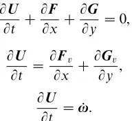
The governing equations for a compressible, reactive flow can be written in conser-vative form in Cartesian coordinates as
∂U
∂t + ∂F
∂x +
∂G
∂y =
∂Fv
∂x +
∂Gv
∂y + ˙ω, (1)
where
U =
ρs ρu ρv ρE
, (2)
F =
ρsu ρu2+p
ρuv u(ρE+p)
, G=
ρsv ρuv ρv2+p
v(ρE+p)
Fv =
−ρsuDs τxx τxy uτxx+vτxy−qx
, (4)
Gv =
−ρsvDs τxy τyy uτxy+vτyy−qy
, (5)
˙
ω = (˙ωs,0,0,0)T. (6)
Here the subscript s denotes a species in the mixture, ρs are the species densities, ρ= PNss=1ρs is the total density of the mixture,u= (u, v) is the bulk velocity of the mixture and uDs = (uDs, vDs) the species diffusion velocities in Cartesian coordinates (x, y),p is the pressure, E the total specific energy of the gas mixture, q= (qx, qy) is the heat flux, and the ˙ωs are the species source terms from the chemical reactions. There are Ns species and thereforeNs species continuity equations.
As usual, the shear stress tensor is given by τxx= 2µ∂u∂x−23∇ ·u, τxy =µ
∂u ∂y +
∂v ∂x
, τyy= 2µ∂v∂y −23∇ ·u, (7) where µis the viscosity of the mixture. The heat flux term for a chemically reacting flow is given by
q=−λ∇T+ Ns X
s=1
hsρsuDs, (8)
where λis the thermal conductivity of the mixture,T is the temperature, and the hs are the species enthalpies.
Equations (1)–(8) give the full Navier–Stokes equations for a compressible, viscous, reacting gas flow. Commonly in numerical studies of this kind with a high-speed flow producing an attached boundary layer, the thin-layer form of the Navier– Stokes equations is used, i.e. Fv is dropped as are terms in Gv which give rise to cross-derivatives. Usually this makes little difference to the results, and is more computationally efficient. However, in this study, as will be seen below, in certain cases the streamwise diffusion must be included, although the cross-derivative terms could have been safely omitted.
The first component of the viscous flux vectors, Fv and Gv, represents the mass diffusion flux of species swhich is assumed to obey Fick’s law, giving
ρsuDs=−µLeP r ∇Ys, (9)
where Ys = ρs/ρ is the species mass fraction. Note that (9) automatically satisfies the requirement PNs
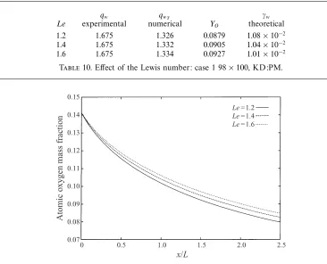
s=1ρsuDs≡0. The Lewis number, Le, is assumed constant for any particular run, but a sensitivity analysis of the effects of a change in Le has been performed, and the results are reported below. The Prandtl number is given by
P r= µcp
λ , (10)
where cp is the mixture specific heat at constant pressure. In this study the Prandtl number is not fixed but calculated from (10).
(a)
Coefficient O O2 Ar
a1 2.6428 3.267 2.5000
a2 −1.7596×10⁻⁴ 1.1324×10⁻³ 0.0
a3 6.075×10⁻⁸ −2.7934×10⁻⁷ 0.0
a4 −5.2372×10⁻¹² 2.5253×10⁻¹¹ 0.0
a5 −5.0993×10⁻¹⁸ 2.0093×10⁻¹⁷ 0.0
a6 2.9215×10⁴ −1.0243×10³ −7.45375×10⁻²
(b)
Coefficient O O2 Ar
a1 2.3584 2.2893 2.5000
a2 8.8833×10⁻⁵ 6.7967×10⁻⁴ 0.0
a3 −9.4390×10⁻⁹ −2.3506×10⁻⁸ 0.0
a4 4.5843×10⁻¹³ 1.1871×10⁻¹³ 0.0
a5 1.7023×10⁻²⁰ −5.3044×10⁻²⁰ 0.0
a6 2.9356×10⁴ 2.8033×10³ −7.45375×10²
Table 1.Thermodynamic curve fit coefficients (in SI units) for (a) 300K < T <5000K,
(b) 5000K < T <25 000K
hence the equation of state for the gas mixture is given by p=
Ns X
s=1
ρsRsT ≡ρR0T
Ns X
s=1
Yi/Ms, (11)
where R = PNss=1RsYs is the gas constant of the mixture, Rs = R0/Ms is the species gas constant, R0 is the universal gas constant, and the Ms are the molar masses of the species.
The temperature is obtained by solving (iteratively) the energy equation E =XNs
s=1
Yshs−RT + 12(u2+v2), (12)
where the species enthalpies,hs, are expressed as a polynomial function of temperature hs =Rs
a1sT+ a22sT2+a33sT3+ a44sT4+ a55sT5+a6s
. (13)
The coefficients in (13) for the O and O2 enthalpy curve fits are obtained from
JANAF thermodynamic data tables (Stull & Prophet 1971) for a temperature range of 300 K to 5000 K (table 1a) and from Balakrishnan (1986) for a temperature range of 5000 K to 25 000 K (table 1b). Thermodynamic data are obtained for Ar from the Chemkin data base (Kee, Rupley & Miller 1987). A similar polynomial expression is obtained for species specific heat at constant pressure (cps) by differentiating the species enthalpy relation with respect to temperature, i.e. cps =∂hs/∂T|p.
3. Transport properties
Species σi (˚A) i/k(K)
O 3.050 106.7
O2 3.467 106.7
Ar 3.542 93.3
Table 2.Lennard–Jones parameters
i.e.
µs= 2.6693×10⁻⁶
√ MsT σ2
sΩµs , (14) where Ωµs is the species viscosity collision integral, σs is the molecular diameter measured in ˚A, and s/k is a reference temperature calculated froms, the depth of the potential well in the Lennard–Jones (12-6) potential, and Boltzmann’s constantk. Species collision integrals are expressed as functions of the reduced temperature
T∗= T
s/k (15)
given by Reid et al.(1977) as
Ωµi =AT∗−B+Ce−DT∗+Ee−FT∗, (16)
where the constants are A = 1.16145, B = 0.14874, C = 0.52487, D = 0.77320, E = 2.16178 and F = 2.43787. This formulation applies to a temperature range of 0.3< T∗<100.
The thermal conductivity for each species is obtained from Euken’s relation (Vin-centi & Kruger 1965) to correct the energy transfer between the internal structure and the translational motion
λs=µs
cvs+94MR0 s
. (17)
The mixture transport properties are calculated using Wilke’s (1950) mixing rule
µ=XNs s=1
µsMYs s
1 PNs
k=1(Yk/Mk)As,k
, (18)
λ= Ns X
s=1
λsMYs s
1 PNs
k=1(Yk/Mk)As,k, (19) where
As,k= 1 2√2
[1 + (µs/µk)1/2(Mk/Ms)1/4]2 [1 +Ms/Mk]1/2 .
4. Surface conditions
of the catalytic material. This reduces to a specific boundary condition for the mass diffusion terms in the viscous flux vector,Gv, at the catalytic wall, given by
µLe P r ∂YO ∂y w =γw
R0Tw 2πMO
1/2 ρwYO,
µLe P r ∂YO2 ∂y w =−γw
R0Tw 2πMO
1/2 ρwYO,
µLe P r ∂YAr ∂y
w = 0,
(20)
whereγwis the catalytic rate coefficient. It varies from zero for a non-catalytic surface through to one for a fully catalytic surface. Note that this is not the only definition that could be used for a fully catalytic wall (see e.g. Anderson 1989), but it is the appropriate one here.
5. Reaction mechanism
A three-species (O2, O, Ar), three reaction mechanism will be used in the gas:
O2+ O2 O + O + O2,
O2+ OO + O + O,
O2+ ArO + O + Ar.
(21)
Given expressions for the forward and backward reaction rates for each reaction, Kfr and Kbr respectively where r is the reaction number, the sum of the rates of production of a species over each non-equilibrium reaction gives the net rate of production of that species, so that
˙
ωs≡ ddρts =Ms Nr X
r=1
(ν0
sr−νsr00) " Kbr Ns Y k=1 ρk Mk ν00 kr
−Kfr Ns Y k=1 ρk Mk ν0 kr# , (22)
where ν0
sr and νsr00 are the stoichiometric coefficients of the reactants and products respectively of species s in reaction r. The sum of the species source terms, ˙ωs, is identically zero.
In the literature a large number of different sets of forward and reverse reaction rate constants, Kbf and Kbr, can be found for oxygen dissociation/recombination reaction schemes, some of which will be considered here. In the problem definition for the Houston workshop (HSFF 1995), forward and backward reaction rate constants were specified in Arrhenius form as
Kf =ATae−Ea/RT, (23)
Kb =BTb. (24)
Reaction A a Ea/R B b
(a) O2+ O2O + O + O2 23.0×10¹⁵ −1 59 400 19.0×10⁹ −12
O2+ OO + O + O 85.0×10¹⁵ −1 59 400 71.0×10⁹ −12
O2+ ArO + O + Ar 3.0×10¹⁵ −1 59 400 2.5×10⁹ −12
(b) O2+ O2O + O + O2 27.5×10¹⁵ −1 59 500
O2+ OO + O + O 82.5×10¹⁵ −1 59 500
O2+ ArO + O + Ar 3.0×10¹⁵ −1 59 500
(c) O2+ O2O + O + O2 32.0×10¹⁵ −1 59 500
O2+ OO + O + O 20.0×10¹⁵ −1 59 500
O2+ ArO + O + Ar 3.0×10¹⁵ −1 59 500
Table 3.Reaction rate constants from (a) the HSFF workshop, (b) Park, and (c) Kang & Dunn.
Ahas units m3mol−1s−1K andBm6mol−2s−1K1/2.
Some of the most commonly used reaction schemes for high-speed, high-temperature flow are those given by Park (1984, 1985). These schemes give the forward rate constants in standard Arrhenius form, and the equilibrium constant, Ke in the form
Ke(T) = exp(A1+A2Z+A3Z2+A4Z3+A5Z4), (25)
whereZ = 10000/T. The backward rate is then calculated from Kb = KKf
e. (26)
For oxygen recombination reactions, as in (22), Park (1985) gives A1 = 8.243, A2 =
−4.127,A3 =−0.616,A4 = 0.093 andA5 =−0.005, whereKehas units m−3mol. Park (1985) gives reaction rate constants for the dissociation of oxygen with molecular and atomic oxygen as the collision partner (the first two forward reactions of (22)), which are similar to the rates given in table 3(a), but not for the third reaction as Park’s reaction schemes do not involve argon. For this reaction we use essentially the same forward rate constant as in table 3(a). With this assumption, the forward rate constants for Park’s scheme are listed in table 3(b).
Park (1984) gives a second set of values for the first two of the forward reactions, quoted from Kang & Dunn (1972). With the same forward rate constant for the third reaction as before, these rate constants are given in table 3(c).
The rate constants given above appear to be essentially for high-temperature flows, particularly for the backward reactions (this will be discussed further below). Chung (1965) gives rate constants for oxygen recombination reactions in the form
Kb =AT−3/2, (27)
where A= 0.4×10¹⁴ or 1.125×10¹⁴m6mol−2s−1K3/2 where, respectively, molecular
most important recombination reaction. Hence the expression given by Chung (1965) for this reaction was used to define an an equilibrium constant in the form
Ke=KfO/1.125×1014T−3/2, (28)
where KfO is a forward rate constant with atomic oxygen as the collision partner. Given a set of forward rate constants, (28) can now be used to calculate the backward rate constants. Alternatively, the backward rate constants given by Chung for atomic and molecular oxygen could be combined with a backward rate constant for argon and then used with a equilibrium constant, e.g (25), to produce a set a forward rate constants. Both of these approaches have been tried.
We now have a number of sets of reaction rates which we could use. However, before continuing it is worth examining in general terms the likely effects of these various sets, particularly as regards recombination of oxygen in the boundary layer, as this will directly affect the heat transfer to the surface in the catalytic region. Park’s scheme (table 3(b) and (25)) gives a forward rate constant of O(10−72) and
a reverse rate constant of O(101466) at 300 K, i.e. in effect no dissociation and an
infinite backward rate giving instantaneous recombination as soon as the gas enters the boundary layer. In this case, there cannot be any surface catalysis as there will be no atomic oxygen in the flow by the time the flow reaches the catalytic region. Further, with reverse reaction rates of this order, there would be no surface catalysis at any realistic flow speed, which is unlikely physically. In contrast, Chung’s expression (27) produces reverse rate constants of O(1010) at 300 K, which would allow a degree of
recombination of oxygen in the boundary layer.
Park (1985) states that the coefficients for the equilibrium constant were obtained from a fit to spectroscopic data at 1000, 2000, 4000, 8000 and 16 000 K. Examination of Park’s fit shows that while lnKe is close to linear inZ for 10006 T 616 000, it rapidly deviates from this for T 61000. This is not surprising as polynomial fits of maximum possible order for the data available are frequently poorly behaved when used for extrapolation. Here, although the coefficient is small, the last term in (25) dominates below 1000 K. A simpler alternative form of Ke consistent with Park’s for 10006T 616 000 was produced by making a linear curve fit to the values produced by (25) at the temperature listed above. The straight line derived gives a very close fit through the data points, with a (negative) correlation coefficient greater than 0.999, and matches the values from (25) closely throughout 1000 6 T 6 16 000, but does not produce unrealistically small values ofKeat low temperatures. This fit is
Ke= exp 10.111−61110/T. (29) Note that, as with Park’s original method, this gives a small activation energy.
Values of the reaction rate constants at 300 and 3500 K, which is basically the range of interest here, with atomic oxygen as the collision partner are given in table 4. The notation for the reaction schemes is H for the HSFF workshop values (table 3a), P for Parks scheme (table 3bor (25)), PM when using the modified form forKe, (29), KD for Kang & Dunn’s values (table 3c), C1 for Chung’s reverse reaction scheme using (28), and C2 for Chung’s scheme using the rate constants given by Chung for molecular and atomic oxygen as the collision partner and backward rate from the Houston scheme for argon. These are combined so that e.g. KD:PM refers to Kang & Dunn for the forward rates andKefrom (29) for the backward reactions.
300 K 3500 K Reaction
scheme Kf Kb lnKe Kf Kb lnKe
H:H 2.9×10−72 4.1×10⁹ −186.86 1.0×10⁶ 1.2×10⁹ −7.06
P:P 2.0×10−72 4.4×101466 −3542.07 9.8×10⁵ 8.3×10⁸ −6.74
P:PM 2.0×10−72 2.4×10¹² −193.59 9.8×10⁵ 1.5×10⁹ −7.35
KD:PM 4.9×10−73 5.8×10¹¹ −193.59 2.4×10⁵ 3.7×10⁸ −7.35
P:C1 2.0×10−72 2.2×10¹⁰ −188.88 9.8×10⁵ 5.4×10⁸ −6.32
KD:C1 4.9×10−73 2.2×10¹⁰ −190.30 2.4×10⁵ 5.4×10⁸ −7.74
PM:C2 1.8×10−74 2.2×10¹⁰ −193.59 3.5×10⁵ 5.4×10⁸ −7.35
JANAF −188.95 −7.09
Table 4.Reaction rate and equilibrium constants for the different schemes with atomic oxygen as the collision partner.
be calculated from knowledge of the basic state of the system under consideration. At equilibrium the forward and backward rates match, and consequently (26) must hold. A standard assumption, used here, is that (26) can be used away from equilibrium to determine forward or backward rate constants given Ke and rate constants in one direction. It follows that any kinetic scheme which does not use or produce a reasonable value of Ke is almost certainly wrong. Calculated values of logKp, where Kp is the equilibrium constant in terms of partial pressure of the components of the gas mixture (hereKp=R0T Ke), are tabulated in the JANAF tables (Stull & Prophet 1971). Note that the formula used to calculate the theoretical values for logKp in the JANAF tables involves logKp rather than Kp, and by convention, equilibrium constants are tabulated in logarithmic form.
From table 4, it appears that apart from the reverse reaction from Park’s original scheme at 300 K, which is clearly wrong, all the reaction schemes produce reasonably consistent values. There is still however considerable variation in the reaction rate constants, reflecting the uncertainty in the values for reactions of this kind. At 300 K, the values of lnKeare, apart from Park’s scheme, within 2.5% of the JANAF values. This is consistent with the difference between the calculated and observed values of logKp given in the sample calculations presented in the JANAF tables. Note in particular that the modified form of Park’s equilibrium constant, (29), produces a reasonable value although it involves extrapolation to a low temperature. There appears to be proportionally more spread in the values of lnKe at 3500 K, although this reflects in part the fact that this is not far from the point where lnKe, or more precisely, logKp, goes through zero.
In summary, it appears that all the sets of rate constants except Park’s original scheme could be used in an attempt to calculate the flows under consideration. Park’s original scheme is still of some theoretical interest as it will produce the case in which there is complete recombination in the boundary layer.
6. Test cases
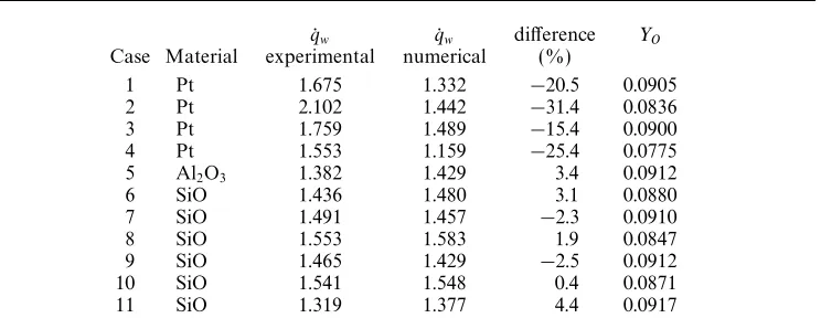
A set of 11 test cases of non-equilibrium laminar flow over a partly catalytic flat plate will be considered. The materials of interest are platinum (Pt), alumina (Al2O3)
U∞ T∞ p∞ qw
Case Material (ms−1) K N m−2 Y
O YO2 YAr 106W m−2
1 Pt 2760 3180 10531 0.142 0.029 0.829 1.675
2 Pt 2740 3180 11997 0.142 0.029 0.829 2.102
3 Pt 2830 3300 11597 0.147 0.020 0.833 1.759
4 Pt 2590 3020 10397 0.119 0.048 0.833 1.553
5 Al2O3 2800 3240 11197 0.147 0.020 0.833 1.382
6 SiO 2790 3240 11864 0.147 0.020 0.833 1.436
7 SiO 2820 3280 11331 0.147 0.020 0.833 1.491
8 SiO 2820 3290 12797 0.147 0.020 0.833 1.553
9 SiO 2800 3240 11197 0.147 0.020 0.833 1.465
10 SiO 2830 3310 12264 0.147 0.020 0.833 1.541
[image:12.595.250.346.470.558.2]11 SiO 2760 3180 10931 0.147 0.020 0.833 1.319
Table 5.Free-stream conditions and the surface heat transfer rate at the catalytic junction
(x/L= 1.8) for the eleven test cases.
species fractions are specified for each test case in table 5, as is the measured value of the heat transfer rate at the catalytic junction. These values have been converted from the form given in the workshop – mole fraction for the species, pressures in mm Hg, andqw at the catalytic junction in cal cm−2s−1 – to the form used in this study, mass fraction, N m−2 and W m−2.
7. Numerical scheme
The numerical scheme adopts a convection–diffusion-reaction operator splitting sequence following Batten et al. (1996) to account for inviscid, viscous and reactive contributions to the flow, giving, in turn,
∂U
∂t +
∂F
∂x +
∂G
∂y = 0, (30)
∂U
∂t =
∂Fv
∂x +
∂Gv
∂y , (31)
∂U
∂t = ˙ω. (32)
The inviscid operator (30) is itself split into one-dimensional equations in the coordinate directions which are then solved using a Godunov-type method (Godunov 1959). The method employs a three-wave HLLC approximate Riemann solver (Toro, Spruce & Spears 1994; Battenet al. 1996). In addition, a MUSCL reconstruction (Van Leer 1979) of the data was used to increase the spatial resolution of the scheme. In an early version of this work, an attempt was made to use the simpler two-wave HLLE (Harten, Lax & Van Leer 1983; Einfeldt 1988) Riemann solver, but this method was discarded due to inaccuracies in the results near the solid wall. In particular, for a flat-plate boundary layer with an adiabatic wall condition, when using the HLLE scheme the calculated recovery temperature on the wall was much larger than expected.
The viscous contribution to the flow was calculated in different ways depending on the problem. The common element was a one-step linearized implicit method for the transverse diffusion terms. Taking Gt as the vector of elements of Gv which contain derivatives in yonly, then the vector of changes to the variables, δU, is given by the solution of "
I −∆t ∂Gˆt ∂U
!n#
δU = ∆tGˆnt, (33)
wheren is the time step,
ˆ
Gnt = G n
t j+1/2−Gnt j−1/2
∆yj , (34)
∂Gˆt/∂U is the viscous flux Jacobian, and I is the identity matrix. Following Batten et al. (1996), (33) can be reduced to a set of Ns+ 3 tridiagonal systems of equations which can be solved individually in order, providing account is taken of the coupling between the equations through the boundary conditions, specifically the catalytic wall conditions.
the left by augmenting the Jacobian. For this semi-implicit method, which is similar to the classic leapfrog method, the time step required with the very fine grid used for the fully catalytic case is an order of magnitude smaller than for an implicit scheme in both directions, but at least an order of magnitude larger than for the basic method when the streamwise terms are treated explicitly. However, it has an important advantage over the scheme with a full implicit solution in the streamwise direction in that it uses only local information, and can therefore be implemented in the parallel code with no further communications overheads. In contrast, the scheme with the full implicit solve couples all grid points along a line in the streamwise direction, so that there would be either a drastic increase in communications, or a significant increase in the complexity of the code to implement this scheme in parallel. The results presented below for the fully catalytic wall were produced using the semi-implicit method.
The cross-derivative viscous terms, when included, were treated explicitly, and were added for example to the right-hand side of (33). These terms, however, could have been safely dropped. Even with the fully catalytic wall where the streamwise diffusive effects were important, tests showed that including the cross-derivative terms does not significantly affect the results.
Although there are three species, only one of them, the atomic oxygen fraction YO need be calculated directly in the viscous step. Argon serves only as a collision partner in the reaction scheme, hence its mass fraction will not change, and once the change in YO has been determined, the change inYO2 is known.
Due to possible stiffness in the reaction scheme, an implicit method is required for the reactive contribution. Equation (32) can be linearized to give
I−∆t
∂ω˙ ∂U
n
δU = ∆tω˙n. (35)
This relation is similar to that for the viscous solver (33), although since the source terms ˙ω do not involve spatial derivatives, (35) can be solved at each point indepen-dently. It is assumed here that the reaction-induced changes over time ∆t are small enough that this linearization can be used. For the particular reaction scheme used here, this assumption is valid. In other cases, however, this may not be true. For example, with a reactive air system (Amaratunga 1998) it was necessary to use a full nonlinear implicit method. This is easily achieved by converting (35) to an iterative Newton–Raphson scheme by updating the Jacobian and the right-hand side during each iteration.
There are a number of possible ways of updating the overall solution from the solutions from the separate operators. A standard way is to use a symmetric sequence of the form
Un+2 =L
Grid CFL qw YO
50×50 1.30 1.347×10⁶ 0.0916
50×100 1.30 1.328×10⁶ 0.0903
98×50 1.30 1.350×10⁶ 0.0917
98×100 1.30 1.332×10⁶ 0.0905
98×200 1.30 1.323×10⁶ 0.0900
Table 6.The surface heat transfer rateqw and atomic oxygen mass fractionYO atx/L= 1.8 cm
for different grids with non-catalytic case 1. The chemistry is KD:PM.
and the variables then updated using
Un+1=Un+δU
Cx+δUCy+δUV+δUR, (37) which requires only two temperature calculations to advance the solution by 2∆t. Both sequences were tried and no significant differences were found. Hence, the cheaper, non-symmetric sequence (37) was used for the results presented below, except in the case when the wall was fully catalytic, when the symmetric sequence was used, although more for reasons of numerical stability than accuracy. We note, however, that this sequence may not always be suitable. In particular, it was found that in certain cases with a reactive air scheme the tighter coupling in the symmetric scheme (36) was required (Amaratunga 1998).
The time step for the scheme is dictated by the stability requirements of the explicit inviscid solver. An artificial Courant number of 1.3, based on the minimum cell length and the maximum wave speed returned by the Riemann solver, was used to set the time step for most of the runs. The exception to this was with the fine grid runs for the fully catalytic case, when the Courant number was set to 0.1 with the semi-implicit scheme discussed above. Taking a smaller time step with a fixed grid had a smaller effect than varying the grid (see table 6 below), so for any particular run, a time step close to the maximum possible was used.
Free-stream values are used for the initial conditions, which implies an instanta-neous introduction of the plate into the moving fluid. This required a small step initially, with the artificial Courant number set at 0.25, but this could be increased after a few hundred time steps. The procedure was time marched to a steady state, with the convergence criterion being that the L2 measure of the change in the
den-sity over a complete time step should be less than 10−8. When starting from the
free-stream conditions, convergence was achieved within a dimensionless time of 16. The grid used in the calculations is a stretched Cartesian grid, with grid points clustered in x near the leading edge of the plate, and near the surface in y. The clustering was achieved using a transformation
dzi= 1 +αexp(dη−βη2
Two of the key variables in this study are the mass fraction of atomic oxygen, YO and the dimensional surface heat transfer rate,qw at the junction, x= 1.8 cm. Table 6 gives these values for a number of different grids for case 1 with KD:PM for the chemistry and a non-catalytic surface. From table 6 it can be seen that provided there are at least 100 points in y, the relative change in the solution is less than 1%, while the 50×50 grid will provide acceptable accuracy for checking the general behaviour of the solution, for example with the different chemical schemes. Unless otherwise mentioned below, the 98×100 grid has been used.
Although satisfactory convergence has been obtained, the accuracy of this solution is not guaranteed. The non-catalytic surface heat transfer rate profile was checked by comparing the numerical solution with that produced by the empirical Eckert formula (Eckert 1955) for the surface heat flux for an isothermal flat plate. Excellent agreement was obtained, and the empirical and numerical heat fluxes were graphically indistinguishable on the scale of figure 2 below. Further, excellent agreement has been obtained with experimental results for flat-plate flows for Mach numbers up to 6.85 (Amaratunga 1998).
8. Chemically frozen flow
For reference, and to examine the basic effects of the surface catalysis, first we consider flow in which there are no chemical reactions in the gas phase: specifically, case 1 withKf =Kb= 0 so that the change in the composition of the gas mixture is forced explicitly by the surface chemistry.
The surface heating rate, which is one of the major variables in this problem, is given, with a change in sign, by qy from (8) and (9) at y = 0. It can be split into thermal (qwT) and catalytic (qwC) contributions, given by
qwT =
λ∂T ∂y
w, (39)
qwC = µP rLe Ns X
s=1
hs∂Y∂ys !
w
. (40)
Figure 2 shows qwT and qwC when γw = 10−2, and qw = qwT for the non-catalytic (γw = 0) case. In this case, on the scale used in figure 2, the thermal heat flux for the catalytic case is almost indistinguishable from the surface heat flux of the non-catalytic plate. Also, the heating rate changes discontinuously over a single grid cell at the catalytic junction, which suggests no significant upstream influence from the catalytic region. Examination of the species mass fractions at the wall confirms that this is indeed the case, with YO = 0.1258 atx= 1.8 cm but the same as the specified incoming value of 0.142 to three significant figures at the grid point before. Figure 2 has as its horizontal axis x/L where L is the reference length of 1 cm. All figures presented below will use this reference length. The vertical axis gives the heat transfer rate in W m−2. All values for heat transfer below will use these units or 106W m−2
(which should be clear from the context) and, where convenient, the units will be dropped henceforth.
5
4
3
2
1
0 0.5 1.0 1.5 2.0 2.5
x/L
Surf
ace heat flux (W m
–2)
(×106) Total heat flux Thermal heat flux Non-catalytical heat flux
Figure 2.Total and thermal surface heat transfer rate solution for case 1 with frozen chemistry
and the non-catalytic heat transfer rate solution for the same conditions.Lis a reference length of
1 cm.
temperature gradient near the wall. In contrast, due to the change in composition of the gas mixture, the thermal conductivity decreases, but by less than 5% byx/L= 2.5. These two effects are opposed, but do not cancel each other. The result is a small decrease in the thermal heat flux due to the catalysis. However, this change is an order of magnitude less than the decrease which occurs in this region because of the continuous growth of the boundary layer, which both the catalytic and non-catalytic solutions display. Hence the apparent lack of change inqwT in figure 2 in the catalytic region.
The observation that there is very little change in the thermal component of the surface heat flux may not extend to other, more general, cases. In particular, as will be seen below, there is a much larger difference between the thermal heat transfer rate in catalytic and non-catalytic cases when the boundary layer is not chemically frozen. Also, this agreement may depend on the details of the modelling. A test calculation was performed with λfrozen at its free-stream value, and a significant change inqwT was observed in the catalytic region.
The boundary condition for the mass fraction of O and O2 is discontinuous at
the catalytic junction. As a result, while the mass fractions are continuous there, their slope is infinite. A self-similar analytical model can be derived for the chemical composition in the neighbourhood of the junction which gives the nature of the singularity at the junction. For generality consider the dissociation/recombination reaction mechanism
X2+MX+X+M, (41)
where M is X2, X, or N, and N acts only as a collision partner. Assume that near
the catalytic junction, very close to the surface the temperature, the total density, and all transport coefficients are constant to leading order. Assume also that the flow is given by a simple linear shear flow, so that u=αy, v= 0 whereαis a constant. The species density equation for the atomic componentX becomes
where for generality the chemical effects have been retained. The mass fraction ofX2
can be written as
YX2 = 1−YN−YX, (43)
where YN is constant. With constant density and temperature the source term forX can be written as
˙
wX=a+bYX+cYX2+dYX3, (44)
wherea, b, cand dare constants. The thin-layer equation (42) now becomes ραy∂YX
∂x =
µLe P r
∂2Y
X
∂y2 +a+bYX+cYX2+dYX3. (45)
The boundary conditions are ∂YX
∂y = 0, x−x0<0, ∂YX
∂y =γYX, x−x0>0,
(46)
where the catalytic junction is at x=x0 and
γ=γw
R0Tw 2πMX
1/2ρP r
µLe
w (47)
from (20). Assuming that the mass fraction of the atomic species at x0 is given by
YX =YXJand that there is a continuous change inYXatx0which does not necessarily
display a regular behaviour, we write
YX =YXJ+ηnf(ζ) +· · ·, (48)
where η=x−x0, ζ=y/ηn is of order one andn describes the leading behaviour of
YO at the surface. Equation (45) now becomes ραηnζ[nηn−1f(ζ)−nηn−1ζf0(ζ)] = µLe
P r η−nf00(ζ)+a+bYXJ+cYXJ2 +dYXJ3 +O(ηn). (49) Equating the order of η on the left-hand side to the leading order of η on the right-hand side gives
n= 1
3. (50)
From (49) it can be seen that the leading behaviour of the atomic oxygen composition is η1/3 irrespective of the reaction mechanism, since the dominant terms will always
be the convective and diffusive terms. Introducing the scalings
f(ζ) =κg(z), ζ=lz, (51)
where
κ=γlYXJ and l =
3µLe ραP r
1/3
w , (52) the governing equation for the self-similar solution forx−x0>0 is
g00+z2g0−zg = 0 (53)
and the boundary conditions are
0
–0.01
–0.02
–0.03
–0.04
–0.05
0 0.2 0.4 0.6 0.8 1.0
((x–x0)/L)1/3
YO
w
–
YOJ
Numerical solution Gradient through origin
Figure 3.Plot of (YOw−YOJ) against ((x−x0)/L)1/3 for the numerical surface distribution of atomic oxygen in the discontinuous region.
The problem defined by (53) and (54) is easily solved numerically. The solution shows a simple monotonic increase fromg=−1.065 atz= 0 to the far-field value of zero, which in practice is obtained before z reaches 5.
On the surface for x > x0, the atomic species mass fraction is given by
YX w =YXJ−1.065κ(x−x0)1/3, (55)
whereYXJ is taken to be the free-stream value for YX.
For the specific case considered here, the predicted values for YO from (55) are compared with the values from the numerical solution in figures 3 and 4. Numerically, the first point with catalytic behaviour lies at x/L = 1.8 and the point immediately upstream is non-catalytic. Hence, in practice the transition from non-catalytic to catalytic behaviour at the surface occurs at some intermediate location between these two points which is not determined exactly by the numerical method. Accordingly, the value of x0 used in plotting figures 3 and 4 was found by adjustingx0 until the
plot of (YOw−YOJ) against (x−x0)1/3, (x > x0), gave a straight line through the origin
in the leading region. The value used was x0/L = 1.776, which is located at 0.75 of
the grid step immediately upstream ofx/L= 1.8.
As can be seen from figures 3 and 4 there is excellent agreement between the numerical and analytical predictions of the change in the mass fraction immediately downstream of the catalytic junction, with, not surprisingly, a gradual deviation between the numerical and analytical values further downstream. The agreement found here is extremely good considering the relative coarseness of the grid in the region of the discontinuity in the boundary conditions. The grid step inxatx/L= 1.8 is 0.032L, and from x= x0 to x/L = 1.8 the predicted drop in the value of YO is 0.016, which is more than 10% of its incoming value.
From (20) and (40), the chemical contribution to the surface heat flux is qwC =γw
r R0Tw
0.14
0.13
0.12
0.11
0.10
0.09
0 0.5 1.0 1.5 2.0 3.0
x/L
Atomic o
xygen mass fraction
Numerical Analytical
2.5
Figure 4.Numerical surface distribution of atomic oxygen and the analytical solution in the discontinuous region.
6
5
4
3
2
1
0
1.5 1.6 1.9 2.4 2.5
x/L
Catal
ytic surf
ace heat flux
(×106)
Numerical solution Analytical-1 Analytical-2
1.7 1.8 2.0 2.1 2.2 2.3
Figure 5.Numerical and theoretical catalytic surface heat fluxes. The solid line is the numerical solution, the dashed line uses the density from the non-catalytic solution and the dotted line allows for the change in density due to the change in composition of the gas.
and the numerical value ofρw), (56) can be used to estimate the catalytic contribution to qw, at and downstream of the junction. Figure 5 shows the distribution of qwC along the surface using the same value forx0 as above. The numerical value ofqwC atx/L = 1.8, 4.448×10⁵, is slightly greater than that predicted from (55) and (56),
4.384×10⁵, and, as expected, both are significantly lower than the predicted value of
4.933×10⁵ at x= x
0 because of the rapid change in YO near the junction and the coarseness of the grid there. As can be seen from figure 5, the predicted values ofqwC are consistently lower than the numerical ones.
constant. However, inspection of the numerical solution with catalysis shows that the density varies from that from the non-catalytic solution. This would be expected because of the rapid change in composition of the gas in this region: for a flow past a flat plate, or indeed any attached thin-layer flow, the change in pressure across the boundary layer from the free-stream value would be expected to be relatively small, but since a change in composition in the mass fraction of the gas will generate a change in the mixture gas constant R, there should be a corresponding change in the total density of the gas at the wall. Inspection of the catalytic and non-catalytic solutions showed that while there is a difference in the surface pressures, proportionally it is an order of magnitude smaller that the change in density, and therefore, since the wall temperature is the same, most of the change in density must come from the change in composition of the gas, which produces a decrease inR and an increase in ρ. Hence, by assuming the pressure is the same as in the non-catalytic case, and using (55) to calculate the surface distribution of YO and YO2, ρ can be estimated from the equation of state (11). This calculation has been performed, and, as shown in figure 5, it removes most of the difference between the predicted and numerical catalytic surface heat flux.
As the grid is refined, the effective value for x0 should approach 1.8L, and the
numerical value of qwC at x= 1.8L should approach the predicted value, but should not reach it, since in a small region very close to the junction the streamwise diffusion terms, which are not taken into account in the model, will be significant and will smooth out the abrupt change assumed above. A calculation with a much finer grid near the junction (∆x/L≈2.6×10−5) gaveY
O= 0.1384 atx= 1.8L, a 2% drop from the free-stream value, and qwC = 4.846×10⁵, again 2% below the predicted value. For comparison, the coarse 50×50 grid gave qwC = 4.32×10⁵. Note that although the fine-grid calculation gives better resolution near the junction, it is much more expensive computationally than that for the standard 98×100 grid. The results from the fine grid could have been used for figures 2 to 5, but the standard grid was used instead as it is the one used for most of the calculations/cases, and to demonstrate the quality of the results that can be obtained near the junction with a relatively coarse grid.
So far we have considered non-catalytic and partially catalytic surfaces. Assume now that the surface downstream of the junction is fully catalytic with γw = 1. The theory presented above predicts that qwC at the junction will be 100 times larger than that with γw = 10−2, i.e. 4.933×10⁷, which far exceeds the thermal component obtained from the non-catalytic solution of 1.076×10⁶. Also, from (55), the estimated
distance for YO to drop from its free-stream value of 0.1416 to zero is 1.75×10⁻⁵L, which is much less than the grid step near the junction for the 98×100 grid of 3.2×10⁻²L. Hence, a much finer grid is needed in this case, and it appears likely
that the streamwise diffusion term will play a significant role. The atomic oxygen mass on the surface near the junction is shown in figure 6, and it is clear that there is a significant amount of upstream influence. The results shown are for a grid with ∆x/L ≈ 2.6× 10⁻⁵, but are graphically identical to those found with
∆x/L≈1.1×10−6 . Also shown in figure 6 is Y
O for a calculation for the thin-layer case when the streamwise diffusion terms are dropped, from which can be seen clearly the upstream influence of the diffusion. The numerical solution gave YO≈0.06, and qwC ≈2.1×10⁷ at the junction, both around half the values predicted by the model. Nevertheless, qwC is still easily the dominant part of the surface heat flux in this region.
0.16
0.14
0.12
0.10
0.08
0.06
0.04
0.02
0 –0.010
x/L
Atomic o
xygen mass fraction
–0.005 0 0.005 0.010 Streamwise diffusion No streamwise diffusion
Figure 6.Atomic oxygen mass fraction near the junction withγw= 1. The abscissa isx/L−1.8.
there is a simple shear flow in this region and that all transport coefficient and other parameters in the problem are constant. The problem forYO then reduces to a convection–diffusion problem governed by
∇2Y =βy∂Y
∂x (57)
with surface conditions
∂Y
∂y = 0, x <0, ∂Y
∂y =γmY , x >0,
(58)
whereY isYO with its free-stream value scaled out, there is an unspecified but small scaling and a change of origin in the coordinate system, and β and γm are as yet unspecified generalized shear rate and catalytic efficiency respectively. The conditions used on the other boundaries are
Y = 1 as x→ −∞, (59)
∂mY
∂xm →0 as x→ ∞, (60)
and
∂mY
∂ym →0 as y→ ∞, (61)
0.16
0.14
0.12
0.10
0.08
0.06
0.04
0.02
0
–0.004
x/L
Atomic o
xygen mass fraction
–0.002 0 0.002 0.004 Numerical solution
Model problem
Figure 7.Atomic oxygen mass fraction for the full numerical solution and the analytic model
solution near the junction forγw= 1. The abscissa isx/L−1.8.
a solution in the form of a power series in the distance from the junction, which is a standard way of approaching problems of this kind.
Relating the parameters in (57)–(61) to the original governing equation for YO, we see that
β=2β
0, where β0= ραP rµLe , (62)
and
γm=γ, (63)
where is the small parameter in the mapping (x−x0, y) → (x, y) between the
coordinate systems.
Examination of the numerical solution shows that near the junction β0 =O(1010)
and γ=O(105), and hence if =O(10−5), which is consistent with the results shown
in figure 6, then both β and γm will be O(1). It follows that there will be a balance of diffusive, convective and catalytic effects near the junction. Since β is non-zero, (57)–(61) can be reduced to a single parameter problem with the further mapping (x, y) →β−1/2(x, y), setting β = 1 in (57) and replacing γ
m by γp = γmβ−1/2 in (59). Now
γp=γβ−01/2 (64)
and therefore a value for γp can be obtained directly from the numerical solution to the full problem. There is however considerable variation in the model parameters in the region of the junction as calculated from the full numerical solution: more than 20% in β0 and γ and consequently, more than 10% in γp. The value used, γp = 1.92, was taken from the full numerical solution at the junction. This value lies about the middle of the range of values spanned by γp (1.8–2.0). The solution for YO from the model problem (57)–(63) is compared with that from the full numerical solution in figure 7, where the model coordinates have been scaled by 0=β0−1/2= 3.8×10⁻⁴L, using the value ofβ0 from the full solution at the junction.
The model problem overestimatesYO. This is not surprising sinceβ0 increases rapidly
Case 5 Case 9
Grid Kf:Kb qwN qwE diff (%) qwE diff (%) YO
50×50 KD:PM 1.446 1.382 4.6 1.465 −1.3 0.0924
98×100 KD:PM 1.429 1.382 3.4 1.465 −2.5 0.0912
50×50 KD:C1 1.222 1.382 −11.6 1.465 −16.6 0.1367
50×50 P:C1 1.206 1.382 −12.8 1.465 −17.7 0.1392
50×50 PM:C2 1.203 1.382 −12.9 1.465 −17.9 0.1395
50×50 P:P 1.811 1.382 31.0 1.465 23.6 0.0000
50×50 P:PM 1.520 1.382 10.0 1.465 3.8 0.0718
50×50 H:H 1.170 1.382 −15.3 1.465 −20.1 0.1446
50×50 none 1.152 1.382 −16.7 1.465 −21.4 0.1472
Table 7.Surface values atx/L= 1.8 with different chemical schemes for non-catalytic
cases 5 and 9.qwN is the numerical heat transfer rate andqwE the experimental value.
will overestimate the convective effects ahead of it, and thereby elevate YO near the junction. In general, however, given the simplicity of this model, there is reasonable agreement between it and full numerical solutions, and it is clear that there is a three-way balance between convective, diffusive, and catalytic effects near the junction, with the streamwise diffusion playing a significant role, unlike the situation when γw is small.
The agreement between the results from the model problem (57)–(63) and the full numerical solution could be improved greatly by using a different set of values forγp and0 than those taken directly from the numerical values at the junction: close to
the best fit is given with γp= 2.85 and0 = 7.7×10⁻⁴L.
9. The different kinetic schemes
4000
3000
2000
1000
0.5
x/L
W
all shear stress (N m
–2)
1.0
0 1.5 2.0
Catalytic Non-catalytic
2.5
Figure 8.Wall shear stress for case 1 with KD:PM kinetics. The catalytic and non-catalytic curves are almost indistinguishable on this scale.
kinetics. In fact easily the least favourable comparison for this scheme was for case 9, as given in table 7. Even allowing for the fact that a coarse grid has been used for this comparison (table 7 also includes the values for the 98×100 for KD:PM), it was clear that the KD:PM scheme gives the best agreement between the numerical and experimental results, and it has therefore been used for all the results presented below.
10. Case 1 with chemistry
Calculations were performed for case 1 using the KD:PM kinetic scheme and the 98×100 grid without catalysis and with catalysis with γw = 10−2. Plots of the shear stress, heat transfer rate, and atomic oxygen mass fraction at the wall are shown in figures 8, 9 and 10. The catalysis has no significant effect on the shear stress. As for the case with frozen chemistry, there is in effect a discontinuous change in the surface heat flux and species mass fractions at the junction, with no significant upstream influence. However, unlike in the case with frozen chemistry, there is now a noticeable change on this scale in the thermal component of the surface heat flux in the catalytic region (figure 9). Further, there are less obvious changes in the flow. The dominant chemical reactions in the gas in the boundary layer are recombination reactions (see table 4), which causes a drop in the value of the gas constant R. This in turn, as explained above, leads to an increase in the density. Hence, although the viscous effects will decrease the streamwise velocity u near the wall, the momentum ρu may increase if the chemical reactions are vigorous enough. This happens here, and adjacent to the wall there is a thin sublayer in which the transverse velocity vis negative.
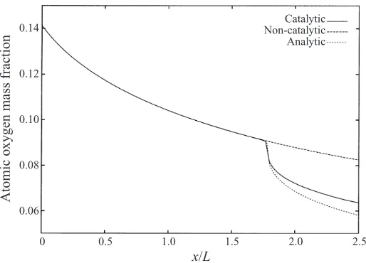
There is a smooth decay inYO(and corresponding growth inYO2) along the wall in the non-catalytic case, but an abrupt change when the catalytic region is encountered. The self-similar model of the behaviour of the solution near the catalytic junction discussed above for the frozen chemistry case can be applied in this case as well, where YOJ is now the value of YO(x0,0) from the non-catalytic solution. In the expansion,
5
4
3
2
1
0.5
x/L
Surf
ace heat flux
1.0
0 1.5 2.0
Total heat flux Thermal heat flux Non-catalytic heat flux
2.5 (×106)
Figure 9.Total and thermal surface heat transfer rate for case 1 with KD:PM kinetics and surface catalysis and the non-catalytic heat transfer rate for the same conditions.
0.14
0.12
0.10
0.08
0.06
0.5
x/L
Atomic o
xygen mass fraction
1.0
0 1.5 2.0
Catalytic Non-catalytic Analytic
[image:26.595.168.425.361.546.2]2.5
Figure 10.Surface atomic oxygen mass fraction for case 1 with KD:PM kinetics.
two terms in the expansion will still be given by (48) withn= 1/3. However, since the base solution is no longer constant, we should not expect such a good comparison between values from the full numerical solution and the analytical solution as shown above when there are no chemical reactions.
4
3
2
1
0
1.6
x/L
Catal
ytic surf
ace heat flux
1.7
1.5 1.9 2.0
Numerical solution Analytical-1 Analytical-2
2.4 (×105)
1.8 2.1 2.2 2.3
Figure 11. Numerical and theoretical catalytic surface heat fluxes. The solid line is from the numerical solution, the dashed line is the basic analytical prediction, and the dotted line includes the effect of the change in density.
the prediction, so that even at x/L = 2.5 there is only 7% difference between the numerical and analytical values ofqwC.
At the junction the non-catalytic solution and (56) predict that the total surface heat flux should beqw= 1.663×10⁶, fromqwT = 1.332×10⁶andqwC = 0.331×10⁶. For comparison, the numerical solution with a catalytic surface producesqwT = 1.304×10⁶ and qwC = 0.301×10⁶, giving qw = 1.605×10⁶, which again is lower than that predicted by assuming no upstream influence. The difference between the numerical and analytical values of qwC is, proportionally, approximately the same as that found for frozen chemistry with the 98×100 grid.
The values obtained for the wall shear stress when the gas mixture is frozen are not significantly different from those shown in figure 8 for the chemically active cases. There is however a noticeable difference between the surface heat transfer rates, as shown in figure 12. Without catalysis, the heat flux is higher when there is chemical activity in the gas. Proportionally this difference increases along the plate, reaching approximately 27% by x= 2.5L. This increase in heat flux is due to an increase in temperature gradient at the surface due to liberation of chemical energy, even though the change in composition of the mixture leads to a drop in the thermal conductivity λ along the plate. In the catalytic region, due to the higher value ofYO, the catalysis has a larger effect when the gas-phase chemistry is frozen, hence the catalytic heat flux is also larger with frozen chemistry. This increase in qwC almost compensates the decrease in the thermal heat flux, so that the total heat flux in both cases is similar in the catalytic region.