Abstract— A non-linear image filtering scheme is described.
The scheme is inspired by the duel domain bilateral filter but owing to much simpler pixel weighting arrangement the computation of the result is much faster. The scheme relies on two principal assumptions: equal weight of all pixels within an isotropic kernel and a constraint imposed on the intensity of pixels within the kernel. The constraint is defined by the intensity of the central pixel under the kernel. Hence the name of the scheme: Intensity Constrained Flat Kernel (ICFK). Unlike the bilateral filter designed solely for the purpose of edge preserving smoothing, the ICFK scheme produces a variety of filters depending on the underlying processing function. This flexibility is demonstrated by examples of edge preserving noise suppression filter, contrast enhancement filter and adaptive image threshold operator. The latter classifies pixels depending on local average. The versatility of the operators already discovered suggests further potentials of the scheme.
Index Terms— Non-linear image processing scheme, local
smoothing with intensity constraint, edge-preserving noise suppression, contrast enhancement, adaptive image thresholding.
I. INTRODUCTION
THE initial stimulus for the development of the proposed scheme arose from the need for noise suppression, edge preserving smoothing filter with a quasi real-time performance. The literature on edge preserving smoothing is plentiful. The most successful methods employ a dual domain approach: they define the operation result as function of “distances” in two domains, spatial and intensity. The “distances” are measured from a reference pixel of the input image. Well known examples are SUSAN [1] or, in more general form, the bilateral filter [2]. The main design purpose of these filtering schemes was the adaptation of level of smoothing to the amount of detail available within the neighborhood of the reference pixel. The application of such schemes ranges from adaptive noise suppression to creation of cartoon-like scenes from real world photographs [3]. The main weakness of the bilateral filter is its slow execution speed due to exponential weighting functions applied to the image pixels in both spatial and intensity domains. There is a range of publications describing the ways of improving the calculation speed of the bilateral filter [4], [5], [6]. In this paper we shall see that the simplification of weighting Manuscript received February 24, 2010. The work is done as part of the development of Pictorial Image Processor© software available at
http://www.pic-i-proc.com.
A. Gutenev is with Retiarius Pty Ltd, PO Box 1606 Warriewood, NSW, Australia, 2102, e-mail: [email protected] .
functions in both spatial and intensity domains not only increases the speed of computation without loosing the essence of edge preserving smoothing, but also suggests a filter generation scheme, versatile enough to produce operators beyond the original task of adaptive smoothing.
II. INTENSITY CONSTRAINED FLAT KERNEL FILTERING SCHEME
A. Intensity Constrained Flat Kernel filter as a simplification of the bilateral filter
The bilateral filter is considered here in the light of its original purpose: single pass application. The output of the bilateral filter [2] is given by the formula [5]
q q p S
q b p b
p
G
p
q
G
I
I
I
W
I
S
R
)
(
)
(
1
, (1)
where
p
andq
are vectors describing the spatial position of the pixelsp
,
q
S
, where S is the spatial domain, the set of all possible pixel positions within the image,Ip and Iq are the intensities of the pixels at positions
p
andq
,I
p,
I
q
R
, where R is the range or intensity domain, the set of all possible intensities of the image,)
2
exp(
2
1
)
(
22
x
x
G
is the Gaussianweighting function, with separate weight parameters σS and σR for spatial and intensity components,
)
(
)
(
p qS q b
p
G
p
q
G
I
I
W
R
S
is the normalization coefficient.
Formula (1) states that the resulting intensity
I
bp of the pixel at positionp
is calculated as a weighted sum of intensities of all other pixels in the image with the weights decreasing exponentially with increase of the distance between the pixel at variable positionq
and the reference pixel at positionp
. The contributing distances are measured in both spatial and range domains. Owing to the digital nature of the signal, function (1) has a finite support and its calculation is truncated to that in the neighborhoods of the pixel at positionp
and intensity Ip. The size of the neighborhood is defined by parameters σS and σR andIntensity Constrained Flat Kernel Image
Filtering Scheme - Definition and Applications
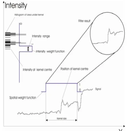
sampling rates in both spatial and intensity domains. The computation scheme proposed below truncates (1) further by giving all pixels in the selected neighborhood the same spatial weight. Furthermore the intensity weighting part of (1) applied to the histogram of the neighborhood is reduced to a range constraint around the intensity Ip of the reference pixel. The idea is illustrated by Fig.1 and Fig 2. For simplicity a single-dimension signal is presented on the graphs. The components which make the output of the bilateral filter (Fig. 1) at a particular spatial position
p
are:i. Part of the signal under the kernel centered at the pixel at
p
,ii. Gaussian spatial weighting function with its maximum at pixel at
p
and “width” parameter σS,iii. Histogram of the pixels under the kernel centered at pixel at
p
, [image:2.595.310.535.212.442.2]iv. Gaussian intensity weighting function with its maximum at Ip and “width” parameter σR
Figure 1 Components making the bilateral filter
The components which make the proposed filtering scheme (Fig. 2) replace the components ii and iv, the Gaussians, with simple windowing functions. The flat kernel works as a spatial filter selecting spatial information in the neighborhood of the reference pixel at
p
. This information in the form of a histogram is passed to the intensity filter, which limits the processed information to that in the intensity neighborhood of the reference pixel Ip . This is where the commonality between the bilateral and ICFK filtering schemes ends. For the ICFK scheme the result of the operation depends on the processing function applied to spatially pre-selected data.
1
)
(
H
),
G(H
1
)
(
H
),
F(H
( )
p p p
p p p
K p ICFK
p
I
if
I
if
I
, (2)
where p
H
is a histogram of the part of the image, which is masked by the kernel χ with the centre atp
,)
(
H
pI
p is the pixel count of the histogram at the level Ip,) (
H
p K p is the part of the histogramH
psubject toconstraint K(p).
Figure 2 Components making the Intensity Constrained Flat Kernel filtering scheme
Introduction of the second function G, applied only when the intensity level Ip is unique within the region masked by the kernel, is a way of emphasizing the need for special treatment of potential outlayers. Indeed, if the intensity level of a pixel is unique within a sizeable neighborhood, the pixel most likely belongs to noise and should be treated as such.
As will be shown below the selection of functions F and G, as well as the constraint K, defines the nature of the resulting filter, which includes but is not limited by adaptive smoothing.
[image:2.595.56.264.335.559.2]A few words have to be said about the choice of the constraint K(p). In the bilateral filter this role is played by the exponent. By separating the constraint function from the processing functions F and G an extra degree of freedom is added to the filtering scheme. One possible definition of K(p)
is offered in Fig. 2, where the exponent is replaced by the window function with a fixed window size.
K(p) = Ip ±, where is a fixed number that depends on the dynamic range of the source image. For example, for integral image types it is an integer.
In some cases, when looking for dark features on a bright background one may want to employ stronger smoothing to the brighter part of the image and reduce smoothing as the intensity decreases. Then the constraint can take the form
K(p) = Ip ± Ip ·, (3) where is a fixed ratio.
Furthermore, one can make the constraint adaptive and for example shrink the domain of the function F as the variance within the area masked by the kernel increases:
K(p) = Ip ±
max
(
max
min)
,where max and min are fixed minimum and maximum
values for the intensity range,
))
H
(var(
min
))
H
(var(
max
))
H
(var(
min
)
var(H
q S
q q
S q
q S
q p
’0
))
H
(var(
min
))
H
(var(
max
q S
q q
S
q ,
)
var(H
p is the variance of the area under the kernel centered atp
.III. OPERATORS DERIVED FROM INTENSITY CONSTRAINED FLAT KERNEL FILTERING SCHEME
A. Edge preserving smoothing filter
This filter can be considered a mapping of the bilateral filter into the ICFK filtering scheme. The functions F and G
are given by the following formulae
) (
H
p K pF
is the average intensity within that part of the histogram under the kernel mask, which satisfies the constraint K(p),
)
H
(
pmedian
G
(4)is the median of the area under the kernel mask.
The median acts as a spurious noise suppression filter. From a computational point of view, the update of the histogram as the kernel slides across the image is the slowest operation. It was shown in [10] that the updates of the histogram and the value of the median for an isotropic kernel can be performed efficiently and require O(r) operations, where r is the radius of the kernel.
The edge preserving properties of the filter emanate from the adaptive nature of the function F. The histogram
H
p is a statistic calculated within the mask of neighborhood χ of the pixel atp
and comprises intensities of all pixels within thatneighborhood. However, the averaging is applied only to the intensities, which are in a smaller intensity neighborhood of
Ip constrained by K(p). Thus the output value
I
pICFK is [image:3.595.305.548.155.402.2]similar in intensity to Ip and intensity-similar features from the spatial neighborhood are preserved in the filter output. If the level Ip is unique in the neighborhood, it is considered as noise and is replaced by the neighborhood median.
Figure 3 Fragment of an underwater image 733 x 740 pixels with a large number of suspended particles
Figure 4 The underwater image after application of the edge preserving smoothing filter with the radius r=12, subject to intensity constraint K(p) = Ip ± Ip • 0.09
[image:3.595.306.548.433.678.2]
perceptually unacceptable noise lumps. Similarly to the bilateral filter, application of the proposed filter gives the areas with small contrast variation a cartoon-like appearance.
B. Contrast enhancement filter for low noise images
The expression (2) is general enough to describe not only “smoothing“ filters, but “sharpening” ones as well. Consider the following expression for the operator function F :
F =
p p p
K p
p p p
K p
I
if
I
if
H
),
max(H
H
),
min(H
) (
)
( , (5)
[image:4.595.46.294.159.446.2]where
H
p is the average intensity of the area under the kernel χ atp
Figure 5 An example of a dermatoscopic image 577 x 434 pixels of a skin lesion
Figure 6 The dermatoscopic image after application of the contrast enhancement filter with the radius r=7, subject to intensity constraint K(p) = Ip ± Ip · 0.03
For the purpose of noise suppression the function (4) is the recommended choice for G in (2). The function F pushes the intensity of the output to one of the boundaries defined by the constraint, depending on the relative position of the reference intensity Ip and the average intensity under the kernel. As any other sharpening operator, the operator (5) amplifies the noise in the image. Hence it is most effective on low noise
[image:4.595.305.549.320.501.2]images. Dermatoscopic images of skin lesions can make a good example of this class of images. Dermatoscopy or epiluminescence microscopy is a technique for imaging skin lesions using oil immersion. The latter is employed in order to remove specular light reflection from the skin surface. This technique has a proven diagnostic advantage over clinical photography [12], [13]. Normally the technique uses controlled lighting conditions. With proper balance of light intensity and camera gain, images taken with digital cameras would have a very low level of electronic noise, while the specular reflection noise is removed by the immersion. An example of such an image is given in Fig. 5. Some of the lesions can have a very low inter-feature contrast. Thus both image processing techniques as well as visual inspections can benefit from contrast enhancement. The images in Fig. 6 and Fig. 7 show application of the filter (5) and clearly indicate that the constraint parameter γ (3) gives a significant level of control over the degree of the enhancement. Another property of this filter that is worth emphasizing is that due to its intrinsic nonlinearity, this filter does not produce any ringing at the edges it enhances.
[image:4.595.47.291.477.660.2]Figure 7 The dermatoscopic image after application of the contrast enhancement filter with the radius r=7, subject to intensity constraint K(p) = Ip ± Ip · 0.1
[image:4.595.312.559.543.751.2]C. Local adaptive threshold
If sharpening could be considered a dual operation to smoothing and a processing scheme producing a smoothing filter is naturally expected to produce a sharpening one, then here is an example of the versatility of the ICFK scheme and its ability to produce somewhat unexpected operators still falling within the definition (2).
Consider a local threshold operator defined by the functions:
F =G=
) (
) (
H
H
,
0
H
H
,
1
p K p p
p K p p
if
if
, (6)
[image:5.595.47.293.486.696.2]where
H
p is the average intensity of the area under the kernel χ atp
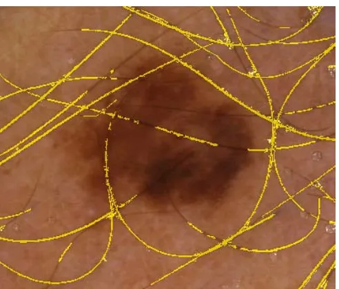
Figure 9 Overlay of direct application of the local adaptive threshold with kernel of radius r= 5 and intensity constraint K(p) = Ip ± Ip· 0.2
Figure 10 Overlay of application of the local adaptive threshold with kernel of radius r=5 and intensity constraint K(p) = Ip ± Ip · 0.2 followed by
morphological cleaning
The operator (6) produces a binary image, attributing to the background the pixels at which local average for the whole area under the kernel χ at
p
is outside the constrainedpart of the histogram. The detector (6) can be useful in identifying the narrow linear features in the images. Here is an example, one of the problems in the automatic diagnosis of skin lesions using dermoscopy is removal of artifacts like hairs and oil bubbles trapped in the immersion fluid. The detector (6) can identify both of those features as they stand out on the local background. Fig. 8 shows the image with the hair. In order to remove the ringing around the hairs caused by sharpening in the video capture device, this image has to be preprocessed with the edge preserving smoothing filter with the kernel radius r=3 and the intensity constraint (3) where γ=0. 08. Direct application of filter (6) gives the combined hair and bubble mask, which is presented as an overlay in Fig. 9. Application of the same filter followed by post-cleaning, which utilizes some morphological operations is presented in Fig 10. The advantage of this threshold technique is in its adaptation to the local intensity defined by the size of the processing kernel.
All ICFK filters described above are implemented and available as part of the Pictorial Image Processor© package
at www.pic-i-proc.com.
ACKNOWLEDGMENT
The author thanks Dr. Scott Menzies from Sydney Melanoma Diagnostic Centre and Michelle Avramidis from the Skintography Clinic for kindly providing dermatoscopic images.
REFERENCES
[1] S. M. Smith and J. M. Brady. “SUSAN – a new approach to low level image processing,” International Journal of Computer Vision, vol. 23, no 1, May 1997, pp. 45–78.
[2] C. Tomasi and R. Manduchi, “Bilateral filtering for gray and color images,” in Proc. of the 1998 IEEE International Conference on Computer Vision, Bombay, India, 1998, pp 839-846.
[3] H. Kang, S. Lee, C. K. Chui. “Flow based image abstraction,” IEEE Transactions On Visualization and Computer Graphics, vol. 16, no 1, January/February 2009, pp 62-76.
[4] F. Durand and J. Dorsey. “Fast bilateral filtering for the display of high-dynamic-range images,” ACM Transactions on Graphics, vol. 21, no 3, 2002, pp 257-266.
[5] S. Paris, F. Durand, “A Fast Approximation of the Bilateral Filter Using a Signal Processing Approach,” International Journal of Computer Vision, vol. 81, no 1, January 2009, pp 24-52.
[6] M. Elad. “On the bilateral filter and ways to improve it,” IEEE Transactions on Image Processing, vol. 11, no 10, October 2002, pp. 1141–1151.
[7] J. Gil and M. Werman, “Computing 2-D Min, Median and Max,” IEEE Trans. Pattern Analysis and Machine Inteligence, vol. 15, May 1993, pp. 504–507.
[8] B. Weiss, “Fast median and bilateral filtering,” ACM Transactions on Graphics (TOG)., vol. 25, Issue 3, Jul. 2006, pp. 519–526.
[9] S. Perreault, P. Hebert, “Median Filtering in Constant Time,” IEEE Trans. Image Processing, vol. 16, Issue 9, Sept. 2007, pp. 2389-2394. [10] A. Gutenev, “From Isotropic Filtering to Intensity Constrained Flat
Kernel Filtering Scheme,” IEEE Transactions on Image Processing, submitted for publication.
[11] M. van Droogenbroeck, H. Talbot, “Fast computation of morphological operations with arbitrary structural element,” Patt. Recog. Letters, vol. 17, 1996, pp. 1451-1460.
[12] H. Pehamberger, M. Binder, A. Steiner, K. Wolff, “In vivo epiluminescence microscopy: improvement of early diagnosis of melanoma,” J. Invest. Dermatol, vol.100, 1993, pp. 356S-362S. [13] S.W. Menzies, C. Ingvar, W. H. McCarthy “A sensitivity and