Abstract— In this paper, we propose a novel ensemble-based approach to boost performance of traditional face recognition methods. The ensemble-based approach is based on the recently emerged technique known as “boosting.” However, it is generally believed that boosting-like learning rules are not suited to a strong and stable learner such as LDA or PCA. To break the limitation, a novel weakness analysis theory is developed in this paper. This theory attempts to increase the diversity between the classifiers train set. For discriminating classifiers in the structure, a train set is divided into some subsets according to dependency or independency of train classes. Then each classifier will be learned on each of these non-overlap train sets. We call a train set is independent (or dependent), if its member, which are face classes, are maximally unsimlar (similar). We use graphs for getting dependent or independent sets of face classes. For combining classifiers, a new unit, which is called “Region Finder”, is introduced. This unit indicates the power of a classifier in the classifier feature space. According to dependent or independent sets, two architectures are proposed which each of them has special characteristics. Promising experimental results obtained on various difficult face recognition scenarios demonstrate the effectiveness of the proposed approach. We believe that this work is especially beneficial in extending the boosting framework to accommodate general (strong/weak) learners.
Index Terms— Face Recognition, Committee Machine, Region Finder, Combining Several Classifiers.
I. INTRODUCTION
FACE RECOGNITION (FR) has a wide range of applications, such as face-based video indexing and browsing engines, biometric identity authentication, human-computer interaction, and multimedia monitoring/surveillance. Within the past two decades, numerous FR algorithms have been proposed, and detailed surveys of the developments in the area have appeared in the literature [1].
Among various FR methodologies used, the most popular are the so-called appearance-based approaches, which include the four most well-known FR methods, namely Eigenfaces [2], Fisherfaces [3], Bayes Matching [4] and ICA [5]. With focus on low-dimensional statistical feature extraction, the appearance-based approaches generally operate directly on appearance images of face object and process them as two-dimensional (2-D) holistic patterns to avoid difficulties associated with three-dimensional (3-D) modeling [6], and
shape or landmark detection [7].
Recently, a machine-learning technique known as “boosting” has received considerable attention in the pattern recognition community, due to its usefulness in designing ensemble-based classifiers [8], [9]. The idea behind boosting is to sequentially employ a base classifier on a weighted version of the training sample set to generalize a set of classifiers of its kind. Often the base classifier is also called “learner.” Although any individual classifier produced by the learner may perform slightly better than random guessing, the formed ensemble can provide a very accurate (strong) classifier.
It is generally believed that boosting-like learning rules are not suited to a strong and stable learner such as LDA or PCA. To break the limitation, several approaches have been proposed for weakening these kinds of strong classifiers. The basic idea in these approaches is to learn each strong classifier with a subset of a train set. Previous methods use techniques such as AdaBoost [10] which gives a distribution to a train set and modifies this distribution in each iteration.
In this paper, we introduce two different approaches for making train sets. These approaches are based on dependencies (or independencies) between face classes in a train set. After dividing a train set to some dependent (independent) subsets, each classifier learns on one of them. For extracting dependent (independent) sets from a train set, we use some graph applications. Also we introduce a new unit which is called “Region Finder” for combining several classifiers. This unit is assigned to a classifier and indicates the distribution of its classifier recognition power in the classifier feature space.
The rest of the paper is organized as follows. Section 2 describes some related works. Section 3 introduces the region finder unit. Section 4 discusses about the dependent and independent train sets. After that, our proposed structures will be introduced in section 5. Section 6 reports experimental results and Section 7 provides a conclusion.
II. PREVIOUS WORKS
Generally, two kinds of ensemble based methods have been proposed for face recognition. The first one is based on a structure of different classifiers and uses whole of a train set for learning each classifier. On the other hand, the second methods use a structure of similar classifiers which each of them is learned on a subset of a train set.
In the first category of ensemble based methods, which are known as face recognitions committee machines, there are
An Ensemble Based Learning For Face
Recognition With Similar Classifiers
several strong classifiers in the structure. Each classifier is a well-known FR method and acts individually. In [11], [12] a structure of five FR classifiers (PCA, LDA, EGB, SVM, and NN) is introduced. In its training phase, each classifier is learned on the train set individually. In the testing phase, after each classifier determines its result, the structure calculates beliefs for each classifier result. These beliefs are calculated in the test phase and according to the classifiers results status. For example, a belief to a classifier result is calculated by counting the number of similar train faces in the first five classifier results. The result, which has the greatest belief, will be selected as the final structure result.
The second category of methods, which contain similar classifiers, emphasizes on using weak classifiers in its structures. LDA is the most familiar FR algorithm which have been tried to be weaken and used in these structures.
The reason behind the LDA selection is that, statistical learning methods such as the LDA-based ones often suffer from the so-called “small-sample-size” (SSS) problem [13]. It is encountered in high-dimensional pattern recognition tasks where the number of training samples available for each subject is smaller than the dimensionality of the samples. A solution for this problem is applying LDA on the some PCA coefficients of train instances. Although this combination of LDA and PCA prevents the SSS problem; But selecting a finite number of PCA coefficients, causes an overlapping problem. Some good ways for avoiding these problems have been proposed by boosting algorithms. In [14], initially, K random feature spaces have been built which each of them contains N0 first principal
components and N1 random principal components. Then in
each feature space, T classifiers learn with the AdaBoost algorithm. The final solution is the combination of K*T classifiers. In [15], a way for weaking LDA classifiers is proposed. In this approach, each LDA is learned with only r train instances for each person (r is less than the number of available train faces for each person).
In this paper, we are interested to improve the second category of FR ensemble methods. The previous works in this category assign a subset of a train set to each classifier which has two characteristics:
a) Each subset contains instances from all face classes. b) The instances in each subset are selected randomly
and they do not have any statistical relation with each other.
We are going to select subsets in a different mode; in such a way that all the instances from a person are located in a subset and classes which are in a subset have a statistical relation with each other (dependency or independency relations). In addition for combining the learners, we propose a new unit which is called “region finder”.
III. REGION FINDERS
In the previous FR ensemble based methods, each classifier is learned on a subset of a train set which includes samples of all train classes. Although accuracy of each classifier in these
structures is limited to the number of instances which are used for learning, but each classifier can recognize samples from all classes individually.
In our approach, a train set is divided into some subsets such that each of them has only instances from one person. So each classifier can recognize test instances from its train set. But for test instances that do not belong to its train set, the classifier finds a class which has the most similarity with the test instance as its result. So if there are n classifiers in the structure, there
will be n non-similar results that one of them may be correct.
For this problem, we need a mechanism for extracting the correct result from the results set. Region finders are placed in the structure for this purpose. If they learn perfectly in the learning phase, they can extract the correct result from all classifier results by weighting the classifier results.
Region finder is a learning agenda which is assigned to each classifier in an ensemble based structure. This unit indicates the distribution of its classifier recognition power in the classifier feature space. A region finder is learned in the training phase. In the testing phase, according to the test instance location in the classifier feature space, it calculates a belief to its classifier result. For example, if a classifier has a high recognition power in a subspace of its feature space and a test instance locates in this area, the belief to the classifier result for this test instance is high.
A region finder, which is assigned to a classifier, learns as following: Instances in the classifier train set with class (+) and other instances with class (-) are used to learn the region finder (For example, the region finder can be a neural network and uses this information for learning).
In a testing phase, in addition to give a test instance to each classifier, it is given to their region finders too. The classifier makes its decision about the class of the test instance and its region finder produces a belief to the classifier result. This belief is proportional to the distance between the test instance and the (+) regions in the classifier feature space.
An important note should be mentioned here is: feature space of a classifier and its region finder must be different (For example a PCA classifier must have a region finder which is learned in a different feature space such as LDA). Selecting the same feature space for a classifier and its region finder causes propagation in error (it will be discussed later).
IV. DEPENDENT AND INDEPENDENT TRAIN SETS
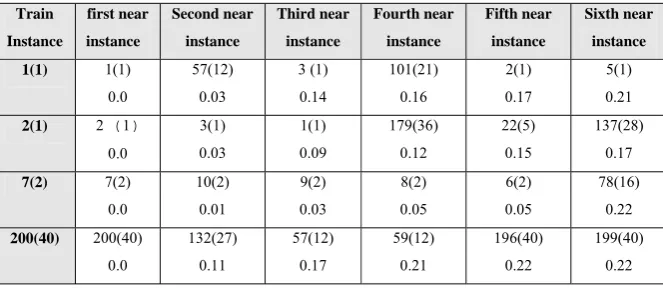
Table 1: A similarity table which shows the result of testing the train faces with a classifier which has been learned before with these train faces. The values in the parenthesizes show classes of
instances. The distances between each instance to a train instance (column 1) is placed in the second raw of each cell.
This table is yielded from testing the train set with a classifier that has been learned before on this train set. With consideration to the similarity table, the following issues can be found:
The first row: the train instance 57 (class=12) and 101 (class=21) are nearer to the train instance 1 (class=1) than train instance 2 (class=1). So there are two train instances whose classes are not 1 (instances 57,101) but are more similar to train instance 1 rather than some instances of class 1 (instances 3, 2, and 5). So we call that classes 1, 12, and 21 are dependent classes. Based on similarities between these class instances, they may make some difficulties for each other in recognition.
The third row: All the instances from class 2 are the nearest instances to each other. Because there is no any instance from class 1 which is nearer to class 2 rather than an instance from class 2, we call that class 1 and 2 are independent classes.
The important note which should be mentioned here is: two classes are independent, if all of their instances are independent but about the dependency between two classes, if only two instances of two classes are dependent, these two classes will be dependent too.
For dividing a train set to some dependent or independent subsets, we use graphs theory. For this purpose, each class in a train set is assumed as one node in a graph. Two graph nodes will be connected, if two classes which are shown with these two nodes are dependent. This graph is called “dependency graph”.
For finding independent train sets, a graph coloring approach is applied on the graph.The aim in a graph coloring problem is assigning a color to nodes such that all two nodes which are connected to each other have two different colors. The number of colors must be a minimum one. Graph coloring problem is a NP-Complete problem and so many approaches have been proposed for it such as simulated annealing [16], Tabu search [17], and DStar [18].
Most of these methods are too slow. We use a simple greedy approach that is not optimal, but it is too fast.
For finding dependent train sets, the largest connected sub graphs are separated from the dependency graph. The approaches which act based on prefix or postfix search can be used here.
V. PROPOSED ARCHITECTURES
We propose two structures in this paper. In the first structure, there are some classifiers which are learned on independent sets which are called independent classifiers. On the other hand, some dependent classifiers are placed in the second structure. The learning and testing process for these structures are similar. The training algorithm is as following:
1. Extract independent (dependent) subsets from the train set. (K is the number of subsets).
2. Arrange K classifiers in the structure which each of them is learned on an independent (dependent) train set.
3. For each classifier, learn a neural network as its region finder. First convert each instance to the region finder feature space. Then assign (+) to the faces which belong to the classifier train set and (-) to other train faces.
And the algorithm which is used for the testing phase is: 1. Give a test face to each classifier and get each classifier result.
2. Give the test face to each classifier region finders and get beliefs to the classifier results.
3. Select the result which has the highest belief among the classifier result as the structure result. This work is done with the gating network.
Although these two approaches have similarities in their algorithms but there are some differences in their structures. The structure and characteristics of each approach are discussed in the following.
VI. ARCHITECTURE I: AN ENSEMBLE OF INDEPENDENT CLASSIFIERS
Some classifiers which are learned in an independent set are arranged in this structure. Remember that an independent Train Instance first near instance Second near instance Third near instance Fourth near instance Fifth near instance Sixth near instance
1(1) 1(1)
0.0 57(12) 0.03 3 (1) 0.14 101(21) 0.16 2(1) 0.17 5(1) 0.21
2(1) 2 (1) 0.0 3(1) 0.03 1(1) 0.09 179(36) 0.12 22(5) 0.15 137(28) 0.17
7(2) 7(2)
0.0 10(2) 0.01 9(2) 0.03 8(2) 0.05 6(2) 0.05 78(16) 0.22
200(40) 200(40)
set is a set whose classes are not similar with each other. So in this structure, each classifier can recognize perfectly a test instance whose class is in its train set. This structure is shown in fig 1. For a test face, each classifier selects one of its train classes as a result. According to the independency between classifiers train sets, we can be sure about the presence of the correct result among classifier results. Region finders must adjust beliefs to the classifier results such that the correct result gets the highest belief.
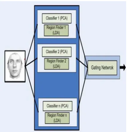
[image:4.595.57.270.245.466.2]As mentioned before, region finders and classifiers must be learned in different feature spaces. For example, in our structure, classifiers use PCA feature space and region finders use LDA one.
Fig 1: The structure of the first proposed Architecture
For explaining the reason for this issue, consider the following scenario: Assume a single PCA classifier recognizes a test face X, whose class is A, as a member of class B. According to dependency between class A and B, they are recognized in two different classifiers. So the result A and result B are in the classifier results set. If region finders are learned in the PCA feature space, a region finder that is assigned to the classifier whose result is B indicates the highest belief and class B is selected as the final result. So there is no any improvement in the structure in compare to a single PCA. On the other hand, if region finders are learned in a LDA feature space, the error will not be propagated (Because the dependencies between classes are not similar in different feature spaces). By decreasing the dependency in classes with using two different feature spaces, the structure improves the performance.
V.II ARCHITECTURE II: AN ENSEMBLE OF DEPENDENT CLASSIFIERS
In the second structure, each classifier is learned on a dependent training set. In a dependent set, there are classes which are similar to each other. In the first structure, each
classifier can recognize easily on its train set and region finders must make a hard decision to find a classifier whose result is correct. But in this structure, the role of classifiers and region finders are inversed. Classifiers decides between dependent classes, that is a hard work and region finders only select the classifier which has all candidate results for a test instance. For this reason, classifiers must use a feature space that:
- It is different from its region finder feature space (For avoiding error propagation).
- It should emphasize on increasing the between-classes distances.
According to these characteristics, dividing a train set between dependent sets and learning region finders do in PCA feature space but classifiers use LDA feature space. LDA feature space in addition to increase the between-classes distances, decreases within-class distances. The structure of this approach is shown in fig 2.
Fig 2: The structure of the second proposed Architecture
VI. EXPERIMENTS AND RESULTS
For evaluating the performance of our proposed structure, we set some tests which each of them evaluate one aspect of our method.
A. Data Set
B. Evaluating the structure performance
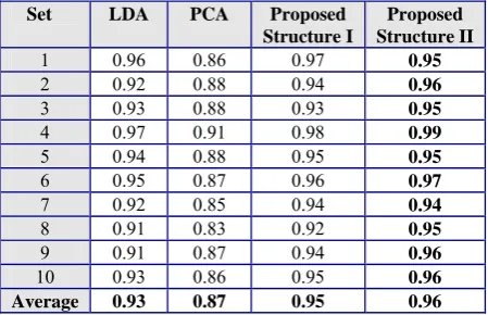
[image:5.595.51.276.253.398.2]For evaluating the performance of these structures, the recognition rate of these two structures and each method which is contributed in these structures (PCA, LDA) were compared on the defined data sets. The results are shown in table 2. According to the table, the improvement of PCA classifiers is obvious. For analyzing results between the LDA and our structures, we define a measure as following: “Similar incorrect instances” is a measure which indicates how much incorrect recognized test instances are similar between the LDA and one of our structures.
Table 2: The comparison of our structures performance with the PCA and LDA classifiers
Set LDA PCA Proposed Structure I
Proposed Structure II
1 0.96 0.86 0.97 0.95
2 0.92 0.88 0.94 0.96
3 0.93 0.88 0.93 0.95
4 0.97 0.91 0.98 0.99
5 0.94 0.88 0.95 0.95
6 0.95 0.87 0.96 0.97
7 0.92 0.85 0.94 0.94
8 0.91 0.83 0.92 0.95
9 0.91 0.87 0.94 0.96
10 0.93 0.86 0.95 0.96
Average 0.93 0.87 0.95 0.96
This measure is important, because in addition to recognition improvement in our methods in comparison with LDA, the low value of this measure indicates a different action between these structures and a single LDA classifier. If this value between two classifiers is near to one, they will have two similar sets of correct and incorrect recognized instances and it can be said that they act similar. This value between LDA and structure I is 0.52 and between LDA and structure II is 0.49. These values confirm that the proposed structures act differently in compare with LDA.
C. Evaluating the effect of the number of train faces on the performance
The number of train faces is an important factor which influences the performance of each FR methods. Generally a large number of training faces increases a FR method performance and vice versa about the small number of train faces. For evaluating this factor, we produced 9 couples of train/test sets of the ORL database. For the couple number n, n/10 of ORL are assigned to the train set and remaining faces
assigned as the test set (n=1... 9). The results can be found in table 3.
By considering to the table, it is obviously clear that our structures can stand more in the small number of training instances situations in compare to LDA and PCA methods.
D. The structures beliefs to recognized and not recognized instances
Our proposed structures have an additional property in compare to single classifier. It can be assign an accurate
belief to each structure result. So if the classifier is not able to recognize a face correctly, it can be found with considering to result’s belief.
In Table 4 and 5, we calculated the average of result beliefs for recognized and not recognized faces in these structures. This feature gives an opportunity to these structures to use other mechanism for judging about the low belief test instances.
Table 3: Comparing the train number on the performances of PCA, LDA and our proposed methods.
Set LDA PCA Proposed Structure I
Proposed Structure II
1 1 0.9 1 1
2 0.97 0.88 0.975 0.99
3 0.945 0.89 0.96 0.96
4 0.925 0.87 0.955 0.95
5 0.91 0.875 0.955 0.955
6 0.85 0.89 0.94 0.921
7 0.79 0.76 0.89 0.76
8 0.65 072 0.83 0.72
9 0.57 0.65 0.73 0.65
Table 4: The average of the first structure beliefs to recognized and not recognized test faces
Set Recognized faces Not Recognized faces
1 0.71 0.18
4 0.74 0.22
7 0.69 0.21
[image:5.595.326.540.445.505.2]Average 0.71 0.20
Table 5: The average of the second structure beliefs to recognized and not recognized test faces
Set Recognized faces Not Recognized faces
1 0.76 0.20
4 0.78 0.25
7 0.75 0.21
Average 0.76 0.22
VII.CONCULUSIONS AND FUTURE WORKS
In the proposed structures, we defined two mechanisms to arrange some similar classifiers in a structure and learn each of them on a subset of a train set which contains dependent or independent classes. Also we introduced region finders which indicate the classifier whose result is the final result. The main idea in these methodologies is using two different methods in classifiers and region finders in order to they can promote each other.
In the future, we are going to evaluate some other combination of pair methods in our structures as classifier/region finder. Also we will try to improve the region finders that we can achieve a better performance in proposed structures. If several different methods are proposed for an application, this boosting structure has this ability to apply on it and we are going to find this kind of applications.
[1]W. Zhao, R. Chellappa, P. J. Phillips, and A. Rosenfeld, “Face recognition: A literature survey”, ACM Computer. Survey, vol. 35, no. 4, 2003, pp. 399–458.
[2]M. A. Turk and A. P. Pentland, “Eigenfaces for recognition”, J. Cogn.
Neurosci., vol. 3, no. 1, 1991, pp. 71–86.
[3]P. N. Belhumeur, J. P. Hespanha, and D. J. Kriegman, “Eigenfaces vs. fisherfaces: Recognition using class specific linear projection”, IEEE Trans. Pattern Anal. Mach. Intell., vol. 19, no. 7, 1997, pp. 711–720.
[4]B. Moghaddam, T. Jebara, and A. Pentland, “Bayesian face recognition”,
Pattern Recognition, vol. 33, 2000, pp. 1771–1782.
[5]M. Bartlett, J. Movellan, and T. Sejnowski, “Face Recognition by Independent Component Analysis”, IEEE Trans. on Neural Networks, Vol.
13, No. 6, 2002, pp. 1450-1464.
[6]V. Blanz, T. Vetter, “Face Recognition Based on Fitting a 3D Morphable Model”, IEEE Transactions on Pattern Analysis and Machine Intelligence,
Vol. 25, No. 9, 2003, pp. 1063-1074.
[7]L. Wiskott, J. Fellous, N. Krueuger, and C. Malsburg, “Face Recognition by Elastic Bunch Graph Matching”, Chapter 11 in Intelligent Biometric
Techniques in Fingerprint and Face Recognition, eds. L.C. Jain et al., CRC Press, 1999, pp. 355-396.
[8]Y. Freund and R. E. Schapire, “A decision-theoretic generalization of on-line learning and an application to boosting”, J. Comput. Syst. Sci., vol.
55, no. 1, 1997, pp. 119–139.
[9]R. E. Schapire, “The boosting approach to machine learning: An overview”, MSRI Workshop Nonlinear Estimation and Classification, 2002,
pp. 149–172.
[10]S. Haykin, “Neural Networks: A Comprehensive Foundation”, book,
Prentice Hall PTR Upper Saddle River, NJ, USA, 1998.
[11]T. Ho-Man, M. Lyu, and I. King, “Face recognition committee machine”, IEEE International Conference on Acoustics, Speech, and Signal
Processing, Vol.2, 2003, pp. 837-840.
[12]T. Ho-Man, M. Lyu, I. King, “Face recognition committee machines: dynamic vs. static structures”, 12th IEEE International Conference on
Image Analysis and Processing, 2004, pp. 121- 126.
[13]S. J. Raudys and A. K. Jain, “Small sample size effects in statistical pattern recognition: Recommendations for practitioners”, IEEE Trans. Pattern Anal. Mach. Intell., vol. 13, no. 3, 1991, pp. 252–264.
[14]H. Kong, X. LI, W. Jian-Gang, and K. Chandra, “Ensemble LDA for face recognition”, International conference on biometrics , Hong Kong,
China, vol 3832, 2006, pp.166-172.
[15]J. Lu, K. Plataniotis, A. Venetsanopoulos, and S. Li, “Ensemble-Based Discriminant Learning With Boosting for Face Recognition”, IEEE
transaction on neural networks, Vol. 17, NO. 1, 2006
[16]J. Culberson, F. Luo, “Exploring the k-Colorable Landscape with Iterated Greedy”, Cliques, Coloring and Satisfiability: Second DIMACS
Implementation Challenge, Providence, RI: AMS, 1996, pp. 245-284. [17]R. Deming, “Acyclic orientations of a graph and chromatic and independencenumbers”, Journal of Combinatorial Theory B 26, 1979, pp.
101-110.