EFFICIENT PARTICLE-BASED SIMULATION OF ION CHANNELS

BY

DAVID D. MARREIRO

Submitted in partial fulfillment of the requirements for the degree of

Doctor of Philosophy in Electrical Engineering in the Graduate College of the

Illinois Institute of Technology

Approved

Advisor

I am thankful for my advisor, Dr. Marco Saraniti, whose guidance and support have enabled me to complete this research. I would also like to thank Dr. Shela Aboud for her assistance, as well as my labmates and friends for their opinions and stimulationg discussions. Finally, I would like to thank my family for giving me the opportunity to pursue my education, and the support to successfully complete it.

Page

ACKNOWLEDGEMENT . . . iii

LIST OF TABLES . . . vi

LIST OF FIGURES . . . xi

LIST OF ABBREVIATIONS . . . xii

ABSTRACT . . . xiv

CHAPTER 1. INTRODUCTION TO ION CHANNEL SIMULATION . . . 1

1.1. Ion Channels . . . 1

1.2. Simulation Approaches . . . 2

1.3. Simulation Issues . . . 3

2. SYSTEM COMPONENTS . . . 5

2.1. Aqueous Solutions . . . 5

2.2. Cell Membrane . . . 8

2.3. Ion Channel Protein . . . 11

3. SYSTEM SIMULATION . . . 16

3.1. Particle-Based Computer Simulation . . . 16

3.2. The Computer Model . . . 34

4. VALIDATION OF THE SIMULATION METHODOLOGY . . . 46

4.1. Benchmarks for Bulk Electrolyte Solutions . . . 46

4.2. Benchmarks for Inhomogeneous Systems . . . 58

4.3. Validation of the Force Field Scheme . . . 63

4.4. Validation of the Integration Schemes . . . 75

5. CHARGE TRANSPORT SIMULATION IN ION CHANNELS . 79 5.1. Measurements In Real Systems . . . 79

5.2. Charge Transport Simulation in Ion Channels . . . 83

5.3. Results . . . 93

5.4. Discussion . . . 100

6. CONCLUSION . . . 106

APPENDIX . . . 109

A. PROTEIN DATA BANK . . . 109

A.1. General Description . . . 110

A.2. File Formats and Standards . . . 111

A.3. Example: OmpF Porin PDB File . . . 112

B. THE GROMACS SIMULATION TOOL . . . 114

B.1. General Description . . . 115

B.2. Usage . . . 116

B.3. Some Examples . . . 117

C. HNC ALGORITHM IMPLEMENTATION . . . 121

C.1. The Ornstein-Zernike Equation . . . 122

C.2. The HNC Approximation . . . 123

C.3. Numerical Solution . . . 124

C.4. HNC Computation Example . . . 126

D. ELECTRICAL DOUBLE LAYER CALCULATIONS . . . 127

D.1. The Classical Theory of the Electrical Double Layer . . . . 128

D.2. The URMGC Model for the Electrical Double Layer . . . . 135

BIBLIOGRAPHY . . . 141

Table Page 4.1 Ion Physical Parameters . . . 64 4.2 Ion–Ion Interaction Parameters . . . 64 4.3 Conductivity Computed for Euler, Verlet-like and PC Integration

Schemes. . . 77 5.1 Experimental Data On OmpF Channel Electrophysiology. . . 82 5.2 Diffusion Coefficient Values Used in This Work. The Superscript

’∞_{’ Refers To Infinite Dilution Or Bulk Values, While the Reduced}

Diffusion Value D0 _{Is Taken From [62]. . . . . 91} 5.3 Side Chains and pKa of the Titratable Residues [13]. . . 103

Figure Page 2.1 Geometry and Polarity of a Water Molecule. . . 6 2.2 Hydrogen Bond Between Two Water Molecules. . . 7 2.3 Schematic Structure of a Phospholipid Molecule. . . 9 2.4 Chemical Structure of Palmitoyl-Oleyl-Phosphatidylcholine and

Schematic Representation. . . 10 2.5 Self-Organized Lipid Nanostructures. . . 10 2.6 Molecular Structure of a Generic Amino-Acid. . . 12 2.7 The OmpF Porin Channel FromE. Coli, Embedded In an Explicit

POPC Membrane (A), and the Corresponding Top View of the OmpF Alone (B). The Picture Is Rendered With VMD [20] From

the PDB Database Structure File 2omf.pdb [21, 22] . . . 15 3.1 Flowchart of a Particle-Based Simulation. . . 19 3.2 Charge Assignment Schemes Used for the PM Force Computation. 20 3.3 Steady-State Ionic Energy of a 0.30 mol.L−1 _{KCl Solution Obtained}

With Euler, Verlet-Like and Predictor/Corrector Integration Sche-mes, for Different Timestep Values Between 1 and 200 fs, Compared

to the Theoretical Value for the Kinetic Energy. . . 31 3.4 Portion of the Finite Difference Grid Used To Solve Poisson’s

Equa-tion. Points Labeled Withn, s, e, w, f, b Are Neighbors of the Point Labeled c, i.e. the Center of the Central Cell. The Points Shown With Primes (n0_{, s}0_{, e}0_{, w}0_{, f}0_{, b}0_{), Are Used for Interpolations.}

Char-acteristics Distances Are Also Depicted (Deltas). . . 44 3.5 Pointers To Nearest Neighbors for the Dirichlet and the Neumann’s

Boundary Conditions. . . 45 4.1 Relation Between RDF and Ion Distribution in a Homogeneous

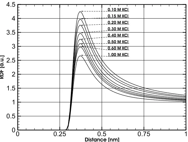
Me-dium. . . 49 4.2 RDFs Between K+ _{and Cl}− _{for KCl Solutions With Concentrations}

Ranging From 0.10 To 1.00 mol.L−1_{. The HNC Algorithm Has Been}

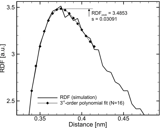
Used With a Lennard-Jones Potential. . . 50 4.3 RDF Curve and 3rd_{-Order Polynomial Fit, From a 0.30 mol.L}−1 _KCl

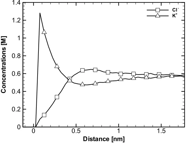
4.5 Ionic Concentration Profiles Obtained from the Simulation of a

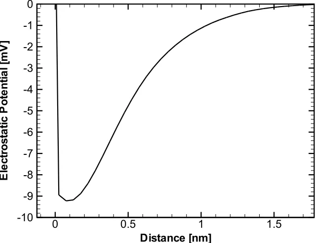
0.5 M KCl Solution in the Vicinity of a Membrane. . . 61 4.6 Mean Electrostatic Potential Obtained from the Simulation of a

0.5 M KCl Solution in the Vicinity of a Membrane. . . 62 4.7 Simulation Results Obtained for the Grid Size ∆GRanging Between

0.30 and 5.0 nm. The Dashed Lines Represent the Benchmark

Val-ues [54]. . . 65 4.8 Simulation Results Obtained for the Free-Flight Timestep ∆tff

Ranging Between 1 and 75 fs. The Dashed Lines Represent the

Benchmark Values [54]. . . 67 4.9 Simulation Results Obtained for the Poisson Timestep ∆tPoiss

Rang-ing Between 0.1 and 30 ps. The Dashed Lines Represent the

Bench-mark Values [54]. . . 69 4.10 RDF for Different Concentrations of KCl and NaCl. Comparison

With Results From the HNC Analytical Model (Solid Lines) Shows

Excellent Agreement [29]. . . 71 4.11 Osmotic Coefficient Versus Concentration for (a) KCl and (b) NaCl

[29]. Results Are Compared With Experimental Values and With Results from the HNC. The Experimental Results Shown Here Use Pitzer Experimental Fit Equations [38] With Parameters Taken from

[55]. . . 72 4.12 Average Concentration of Anions and Cations in a 0.15 mol.L−1 _KCl

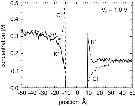
Solution With a 2 nm Dielectric Membrane in the Center [29]. . . 73 4.13 Average Concentration of Anions and Cations in a KCl Solution

With a 2 nm Dielectric Membrane in the Center. The Concentra-tions Are 0.30 mol.L−1 _{On the Left and 0.15 mol.L}−1 _{On the Right}

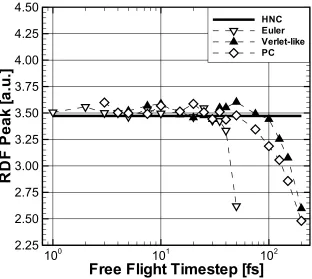
Side [29]. . . 74 4.14 Comparison of Different Integration Schemes Over a Range of

Inte-gration Timesteps. The RDF Peak Value for a Bulk KCl Solution of 0.30 M Is Used as a Benchmark and Compared to the Analytical

HNC Result [54]. . . 76 4.15 DL Potential Drop for Various KCl Concentrations, Obtained With

All Three Integration Algorithms, Compared With the URMGC Analytical Predictions. An Integration Timestep of 20 fs Is Used in

the BD Simulations. . . 78

MGC Analytical Results. An Integration Timestep of 20 fs Is Used

in the BD Simulations. . . 78 5.1 Patch Clamp Measurement Setup With Op-Amp Voltage Clamp and

Current Amplification [3]. . . 80 5.2 System Model Schematic Showing Geometry and Boundary

Condi-tions. . . 85 5.3 Map of Potential and Force Experienced By a K+ _{Ion Along a Plane}

Perpendicular To OmpF Pore Axis. . . 87 5.4 Map of Potential and Force Experienced By a Cl− _{Ion Along a Plane}

Perpendicular To OmpF Pore Axis. . . 87 5.5 Minimal Potential Path for K+ Ion Along Porin Channel Pore. . . 88 5.6 Potential Profile for a K+ _{Ion Along the Minimum Constraint Path}

in the Porin Channel Pore. . . 89 5.7 Pore Openings Model and Current Recording Procedure. . . 90 5.8 Porin Trimer Conductance As a Function of the Free-Flight

Inte-gration Timestep, Compared With an Experimental Measurement (Dashed Line) [59]. The Bath Concentration Is 1.00 M and the

Applied Trans-Membrane Potential Is 0.5 V. . . 93 5.9 Dielectric Map of the Protein Area As Represented in the

Simula-tion. Section Along y₋z Plane, A) Without Smoothing, B) With

Smoothing. protein Is Set To 6 in Both Cases. . . 95 5.10 I-V Curves Obtained With a Smoothed Dielectric Representation,

With a 0.25 M KCl Bath and Applied Trans-Membrane Potentials Varying Between ₋200 and +200 mV. Diamonds: protein = 5,

Tri-angles: protein = 20. . . 96 5.11 Channel Conductances Due To K+_{, Cl}−_{, and Trimer Total}

Conduc-tance As a Function of the Protein Relative Dielectric. The KCl Concentration Is Set to 0.25 M and the Trans-Membrane Voltage Is

500 mV. . . 97 5.12 Trimer Conductance As a Function of Bath KCl Concentration.

Cir-cles: BD Simulation Withprotein = 6, Squares: BD Simulation With

protein = 20, Triangles: PNP Simulation [59], Diamonds:

Experi-mental Measurements [62]. . . 98

lation With Reduced Diffusion D, Triangles: PNP Simulation [59],

Diamonds: Experimental Measurements [62]. . . 100 5.14 OmpF Trimer View Showing Some of the Charged Residues Lining

the Constriction Region (Generated With VMD [20]). . . 102 5.15 Computed Total Net Charge of OmpF As a Function of the pH. . 103 B.1 GROMACS Simulation Results for a Bulk KCl 1.0 M Solution. The

RDF Shows an Excellent Agreement With the HNC Benchmark. . 119 B.2 Map of the Force On a K+ _{Ion Along a Plane Perpendicular To the}

Pores of OmpF Obtained With the GROMACS P3_{M Algorithm,}

Using a Custom Script. . . 120 C.1 RDFs for a 0.15 mol.L−1 KCl Solution Obtained from the HNC

Integral Computation. The Interaction Potential Uses the Empir-ical Lennard-Jones Formula and a Value of 5×108 _{Is Used for the}

Splitting Parameter α. . . 126 D.1 Ionic Concentration Profiles Computed With the Standard DL

The-ory for a 1–1 Electrolyte Bulk Concentration of 0.5 M and a Surface

Potential of 30 mV. . . 131 D.2 Mean Electrostatic Potential Computed With the Standard DL

The-ory for a 1–1 Electrolyte Bulk Concentration of 0.5 M and a Surface

Potential of 30 mV. . . 132 D.3 Charge Accumulation In the DL As a Function of the Bulk

Elec-trolyte Concentration for Values of the Surface Potential Ranging

Between 5 and 150 mV. . . 134 D.4 Potential Drop Across the DL As a Function of the Bulk Electrolyte

Concentration for Values of the Surface Potential Ranging Between

5 and 150 mV. . . 134 D.5 Illustration of the Three Regions Used for the Solution of the

UR-MGC Equations. . . 136 D.6 Ionic Concentration Profiles Computed With the URMGC Model

for a 1–1 Electrolyte Bulk Concentration of 0.5 M and No Surface

Charge. . . 139 D.7 Mean Electrostatic Potential Computed With the URMGC Model

for a 1–1 Electrolyte Bulk Concentration of 0.5 M and No Surface

Charge. . . 140

D.9 Potential Drop Across the DL As a Function of the Bulk Electrolyte

Concentration With No Surface Charge Present. . . 141

Abbreviation Term

AC Alternating Current

AMU Atomic Mass Unit

BC Boundary Conditions

BD Brownian Dynamics

CIC Cloud In Cell

DL Double Layer

DNA DeoxyriboNucleic Acid

E. Coli Escherichia Coli

FMM Fast Multipole Method

GNU Gnu is Not Unix

GROMACS GROningen MAchine for Chemical Simulations

HNC HyperNetted Chain

IP Inverse Power

KCl Potassium Chloride

LJ Lennard-Jones

M Molar [mol.L−1_]

MD Molecular Dynamics

MGC Modified Gouy-Chapman

MSA Mean Spherical Approximation

NaCl Sodium Chloride

NMR Nuclear Magnetic Resonance OmpF Outer Membrane Protein F

OZ Ornstein-Zernike

P3_{M Particle-Particle–Particle-Mesh}

PB Poisson-Boltzmann

PBE Poisson-Boltzmann Equation

PC Predictor/Corrector

PDB Protein Data Bank

PM Particle-Mesh

PNP Poisson-Nernst-Planck

POPC Palmitoyl-Oleyl-PhosphatidylCholine

PP Particle-Particle

PY Perkus-Yevick

RC Resistor-Capacitor

RCSB Research Collaboratory for Structural Bioinformatics RDF Radial Distribution Function

RMS Root Mean Square

TSC Triangular Shaped Cloud

URMGC Unequal Radius Modified Gouy-Chapman VMD Visual Molecular Dynamics

The main objective of this work is to demonstrate the validity of a Poisson Particle-Particle–Particle-Mesh (P3_{M) coupled with a Brownian Dynamics (BD)} en-gine simulation tool in modeling charge transport in biological ion channels. The chal-lenges of ion channel modeling are presented with the underlying physical considera-tions. The details of the P3_{M force field scheme and its implementation are presented.} The BD algorithm and the various integration schemes for the particle dynamics are presented and compared. The numerical model proposed for the electrolyte solution, the membrane and the ion channel are discussed. A set of benchmarks are defined and motivated to validate the numerical representation of the system. Analytical models are proposed for the electrolyte solution in bulk and interfacial conditions: the Hyper-netted Chain (HNC) approximation is used in conjunction with the Ornstein-Zernike integral equation theory to describe the electrolyte solution, and provide a comparison with the simulation results. Similarly, the Gouy-Chapman Double Layer (DL) theory is used to compute analytical benchmarks for the membrane-solution interface simu-lation. The P3_{M BD simulation of bulk electrolyte solutions and membrane-solution} interfaces is validated by comparison with the proposed analytical benchmarks. The range of valid numerical parameters for the system is determined by defining and applying an error analysis methodology. Subsequently, the well-studied OmpF porin channel from bacteriumE. Coli is used as a test case to validate the proposed charge transport simulation approach. Potential mapping of the pore is performed for differ-ent ion types. Dynamic charge transport simulations are performed, and macroscopic channel conductance values are extracted and compared with published experimental measurements as well as other numerical models. The applicability of the P3_{M BD} simulation is discussed, and compared with other numerical models from the com-putational cost standpoint. Finally, ways to improve the algorithmic efficiency and accuracy of the simulation are introduced.

CHAPTER 1

INTRODUCTION TO ION CHANNEL SIMULATION

1.1 Ion Channels

Ion channels are proteins embedded in the lipid membranes of biological cells. The interaction between the channels and their environment is quite complex and is responsible for the regulation of the ionic flux across the membrane. Examples of the crucial biological functions accomplished by ion channels are the generation and transmission of potentials in nerves and muscles, as well as the hormone release from endocrine cells [1].

full understanding of ion channels would allow for the modification of their design for new applications [5] or the manufacturing of analogous structures reproducing their functionalities [7]. These prospects have motivated increasing research efforts especially in the field of computer modeling, due to the availability of reliable protein structural data, reproducible experimental data, and high performing software and hardware computational machinery.

1.2 Simulation Approaches

A hierarchy of simulative approaches have been applied to the study of ion channels during the last two decades. The implemented theoretical models range from the simplest to the most complex and computationally challenging. This section will give a brief classification of those models.

The simplest representation for a membrane–channel system is a simple RC circuit [1], this simplistic approach is able to model some measurements of the tran-sient response of cell membranes to current steps, and helps in characterizing the type and density of ion channels, together with some membrane properties.

The next level of simulation complexity involves the continuum models, such as the Poisson-Boltzmann approach [8] and the Poisson-Nernst-Planck method [9], which have been used to define the electrostatic landscape of ion-channel systems. In these models, the ion electrodiffusion is modeled in terms of continuous fluxes.

On the other hand, particle-based approaches analyze ion fluxes as individual particle trajectories. The particle-based approaches can use either Brownian [10] or Newtonian [11] dynamics to model the trajectories and are the most favored for an accurate yet practical model of ion channels.

description of the atomic interactions and would be very successful in describing the details of the electrostatic and finite-size effects taking place in the constricted pore region. However, this method is still impractical because of the many computational and theoretical challenges which will be briefly introduced in the next section.

The question that may be asked is: why modeling ion channels? While it is true that experimental results have been obtained in an accurate and reproducible way and have provided insight into the inner works of ion channels, while X-ray crystallography has provided increasingly accurate protein structures for a variety of channels, a computer model still permits the realization of experiments otherwise impossible. In a computer model, all the parameters can be easily modified, making a very large variety of experiments possible. Voltages, currents, ion concentrations, temperatures, and every significant physical parameter can be changed to produce the desired experimental setting. Different channel structures can be simulated, mak-ing the prediction of the behavior of mutants [7] or man-made nanotubes [12] and other channel-like structures possible. Finally, the biggest advantage of computer experiments is that results are obtained at different modeling levels, allowing the reproduction of macroscopic voltages and currents as well as the details of atomic interactions and trajectories. No real physical experiment is currently capable of ac-cessing that kind of information, hence the increasing interest for computer models.

1.3 Simulation Issues

The second challenge is the nature of the phenomenon of ionic charge transport itself. Most of the physics defining the characteristics of the transport occur in the confined pore region, over distances measured in ˚Angstroms. The complete charge transport process is measured in microseconds, yet the ion transport in the pore itself relies upon atomic motion details occurring in fractions of a femtosecond. A model that is successful in describing ionic transport in an ion channel system must therefore be able to model the entire system for a long time, while at the same time following the system dynamics with space and time resolution of fractions of ˚A and femtoseconds, respectively.

Therefore, the simulation of ion channels demands for very efficient computer algorithms. This work is devoted to the development and improvement of particle-based computer simulation algorithms for the study of ionic channel transport prop-erties.

CHAPTER 2 SYSTEM COMPONENTS

Ion channels serve as an interface between two different media in biological cells. They naturally embed themselves in the cell membrane separating the inside and the outside of the cell, and allow ions in or out under specific conditions. A study of ion channels has therefore to include all three elements (aqueous solution, membrane, ion channel) in their natural configuration. This chapter will describe in detail the nature and the physics of each component of the system: the aqueous solutions, the membrane, and the ion channel protein itself.

2.1 Aqueous Solutions

A comprehensive study of the physics of electrolyte solutions is a strong pre-requisite for any work related to biological systems. This is for a very simple reason: all living creatures and their constitutive tissues are composed mostly of water [13]. Hence the most common medium encountered in these studies will be aqueous solu-tions composed of water and ions.

Water has a very particular set of physical characteristics which play an im-portant role in many biological functions. The components of living cells interact extensively with water, and this interaction determines their shapes and character-istics. Water is a source of mechanical stability for biomolecules and much of the metabolic reactions and processes occur in an aqueous environment. Ion channels do not derogate from this rule, since their function is to actually connect two separate electrolyte solutions.

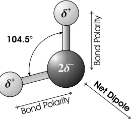
symmetric because of the difference in the electronegativity of oxygen and hydro-gen. Electronegativity is the tendency for atoms to attract electrons. Oxygen is very electronegative in comparison to hydrogen, which tends to lose its electron, forming a simple proton (H+_{). The resulting O–H bond is therefore polarized, since the electron} pair is on average located closer to the oxygen atom than the hydrogen. This results in a partial positive charge δ+ _{on each H and a negative charge 2δ}− _{on the oxygen.}

By itself, this property of the bonds does not explain the polarity of the water molecules. The permanent electrostatic dipole of the water molecule comes from the misalignment of the two O–H bonds. The two covalent bonds make an angle of 104.5◦ _{and their polarities form an electrostatic dipole (Figure 2.1) [13]. Water is} therefore a polar solvent and any other compound with a net electrostatic dipole will be easily soluble in water. Examples are ammonia and ethanol, both of which have dipoles from polarized N–H and O–H bonds. The substances that readily dissolve in water are called hydrophilic. On the contrary, molecules that exhibit little or no polarization like hydrocarbon chains are less soluble in water, and are then qualified as hydrophobic.

104.5°

d+

2d- Bond P

olarity

Bond Polarity Ne

t D_ip ole d+

Figure 2.1. Geometry and Polarity of a Water Molecule.

weak bond between them (Figure 2.2). This bond is called the hydrogen bond [13], and each water molecule can form up to four bonds with four neighbors. Hydrogen bonds are longer than the covalent O–H bond, and much weaker. The energy required to break a hydrogen bond is about 20 kJ mol−1_{, while breaking the O–H bond takes} 460 kJ mol−1_{. In ice, each molecule is hydrogen-bonded to its four neighbors resulting} in a regular hexagonal lattice structure. These bonds give ice its high melting point and rigidity. In liquid water however, hydrogen bonds continuously break and reform, making it fluid.

d+

2d

-d+

d+

d+

0.10 nm

0.18 nm

Hydrogen Bond

2d

-Figure 2.2. Hydrogen Bond Between Two Water Molecules.

K+_–Cl− _{electrostatic interaction and allow the ions to separate and move freely in} the solution. This dissolution process continues until an equilibrium is reached. At that point the solution is saturated, i.e. there are enough free ions in the solution to screen the effect of water on the remaining crystals, preventing their dissolution. Typical saturation concentrations do not occur normally in biological systems, and the next sections will focus only on moderately concentrated ionic solutions.

2.2 Cell Membrane

The boundaries of cells are formed by biological membranes preventing mol-ecules inside to leak to the outside, and also unwanted substances from the outside to enter the cell. Cell membranes contain transport systems to control the flow of chemicals in and out of the cell. Some of the transport processes are produced by ion channels. To better understand how the channels are inserted in the membrane, and how the membrane structure is stabilized in water, it is important to understand the chemistry of the membrane molecules themselves.

Biological membranes are composed of lipid molecules. This class of substances contains three major types of molecules, of which the phospholipids are the most important. The other two groups, glycolipids and cholesterol realize some specific functions and are not as abundant in cell membranes. This section will elaborate on the molecular structure of phospholipids, and how they assemble to build cell membranes.

molecule through a phosphate group. Figure 2.3 shows the schematic structure of a phospholipid [15].

Fatty acid

Fatty acid

Alcohol

Glycerol

Phosphate

Figure 2.3. Schematic Structure of a Phospholipid Molecule.

The phospholipids therefore share the same common structure, with two apo-lar hydrocarbon chains forming the hydrophobic side of the molecule, and a strongly polarized and hydrophilic side with the charged phosphate and amine groups. Within the phospholipid group, thepalmitoyl-oleyl-phosphatidylcholine (POPC) is one of the most commonly found in the membranes of bacteria like E. Coli. This work will use POPC molecules as building blocks of the cell membrane for the systems stud-ied. Figure 2.4 shows the complete chemical structure of a POPC molecule and its schematic representation.

P O

CH3

N +

_ O

C

O O

C

O O

O

O CH3

CH3 Fatty acids Glycerol Phosphate Choline

Schematic representation

Figure 2.4. Chemical Structure of Palmitoyl-Oleyl-Phosphatidylcholine and Schema-tic Representation.

Micelle Bilayer

Figure 2.5. Self-Organized Lipid Nanostructures.

potential. These trans-membrane potentials play a role in the ionic transport across the membrane through the channels.

2.3 Ion Channel Protein

Ion channels perform many highly specialized functions in cells. They are therefore classified in a number of families depending on which kind of ions they transport. Ion channels present three main properties: the permeation is the abil-ity to allow ions to cross the strong dielectric barrier due to the lipid membrane, the selectivity is the capability of selecting one specific type of ions and not letting others go through the channel, while gating refers to the ability of the channel of modulating the ionic flow depending on external stimuli such as the trans-membrane voltage or the binding of an activating substance to the channel. This section will describe the chemical structure of ion channels, how they are organized and how they work. Finally, the ion channel used to evaluate the proposed simulation techniques is presented.

2.3.1 Protein Biochemistry. Ion channels are proteins, as such they are large macromolecules synthesized by the cells from small building blocks called amino-acids. All organisms use the same 20 amino-acids as building blocks to assemble their proteins. These 20 amino-acids are derivatives of carboxylic acids and share a common basic structure centered around a carbon atom called the α-carbon. This atom is bonded to an amine group H3N+_{, a carboxylic group COO}−_{, a hydrogen} atom, and a side chain which is different for every amino-acid [13]. Figure 2.6 shows the generic structure of an amino-acid. The side chain is represented by the symbol R.

H N₃ CH COOH R

a

+

Figure 2.6. Molecular Structure of a Generic Amino-Acid.

sequence or the order in which the amino-acids are connected. This sequence is called the primary structure of the protein. The long peptide chain is a succession of molecule elements called residues, coming from the original amino-acids. Each residue presents a side-chain with specific chemical functional groups depending on the original amino-acid. These groups can be polar or apolar, and in some cases bear a net electric charge. Their organization in the chain form the basis for both the structure of the protein and its functionality when side-chains are accessible on the surface of the protein.

Proteins can also exhibit a quaternary structural order. This is the case when several subunits, each made of a single peptide chain, bind together to form the protein. This is the case of the OmpF porin channel described later in this section.

2.3.2 Structure and Function. Ion channel proteins are composed of an arrange-ment of one or more cylinders forming pores that span the membrane. Ions crossing the channel will travel through these pores. While it is clear that the 3D structure of the protein is crucial in defining its function, the various properties of the ion chan-nels such as selectivity or gating involve more complex structural properties than the static shape of the protein. Many ion channels feature a selectivity filter which is the basis of their ability of restricting the ionic flow to a particular ion type. The selectivity filter is usually made by an arrangement of side chains located inside the pore, providing the specific electrostatics and geometry needed to transport some ion species and block others. An accurate knowledge of the protein structure is therefore necessary for the understanding of the ion channel functionality.

The protein structures are obtained through X-ray scattering experiments on crystals of pure proteins. The data collected are correlated to the amino-acid sequence to determine the actual spatial arrangement of the residues and the 3D protein struc-ture. The mapped proteins are available in an open library called the Protein Data Bank (PDB) [18]. Appendix A details the data formats used in the PDB and how to manipulate them to model protein structures in the simulation programs.

-strands. The structure also shows chain loops creating a constriction region inside the barrel. This constriction actually reduces the pore diameter to approximately 6 ˚

Figure 2.7. The OmpF Porin Channel From E. Coli, Embedded In an Explicit POPC Membrane (A), and the Corresponding Top View of the OmpF Alone (B). The Picture Is Rendered With VMD [20] From the PDB Database Structure File

CHAPTER 3 SYSTEM SIMULATION

The goal of a simulation code is to reproduce and predict the behavior and characteristics of a real system by implementing a physical model. The accurate reproduction of time-dependent properties of the system and its response to externally imposed conditions is the desired result of a successful simulation.

3.1 Particle-Based Computer Simulation

The study of microscopic systems such as ion channels involves modeling the behavior in time of the structure and its full environment. In the case of microscopic systems it makes sense to use a particle representation, as the system is naturally divided into molecules and atoms, i.e. “particles”, which are subunits suitable for a numerical representation. The whole system is then represented by a set of particles interacting with each other and with their environment. For instance, the E. Coli OmpF membrane channel in its biological environment contains 10,344 atoms [21], and a complete simulation must include the membrane molecules, the solvent, and the ions, raising the total number of simulated particles to hundreds of thousands.

The particle-based simulation tool described in this work is self-consistent. This means that the forces due to the interactions between the components of the system strictly depend on the spatial configuration of the components themselves. Therefore, the position of the particles and the force field they generate must be updated as the dynamics of the system evolves during the simulation.

in a computationally efficient manner. In particular, these interactions are expressed by electrostatic forces generated by charged particles or externally applied fields, by non-electrostatic forces such as van der Waals forces (see Section 3.2.1.1), or by chemical bonding.

The simplest way to compute the total electrostatic force acting on a particle is to loop over all the charged particles within the system, and determine for each one the influence of every other particle. This process is implemented in the so-called Particle–Particle (PP) algorithm, scales as N2 _{[23], and its computational cost is} prohibitive in the case of biological systems because of the long-range nature of the electrostatic interactions and the resulting large number of neighbors needed to be accounted for in the force calculation. Therefore, other approaches must be employed to produce a computationally efficient model.

The option we have chosen is therefore to combine the PP and PM methods in a unified Particle-Particle-Particle-Mesh (P3_{M) algorithm. Two main methods have} been proposed for the computation of the force field schemes in biological systems. They are the Fast Multi-pole Method (FMM) [24, 25] and the P3_{M method [23].} The latter option has been chosen because it has the ability to efficiently model the electrostatics of inhomogeneous systems with arbitrary boundary conditions. The Ewald summation method [26] solves the PM component in reciprocal space. One of the requirements for the Ewald method is the spatial periodicity of the charge distribution, which is at odds with the inhomogeneous nature of the ion channel systems. Studying ion channels requires the ability to handle non-periodic boundaries with externally applied potentials, which is incompatible with the Ewald method [27]. On the other hand, a real space Poisson solver easily fulfills these requirements. Even though the use of this technique has been limited in the past due to the assertion that the self-consistent solution of Poisson’s equation in particle-based simulation of ion channel systems is computationally prohibitive [28], it was proved to be applicable to this kind of simulations [29].

Within the P3_{M method, the force on each particle is decomposed into two} components [23]:

~

Fi =F~iP M +F~iP P, (3.1) where the long-range component F~P M

i of the total forceF~i on a particle iis obtained from the solution of Poisson’s equation on a grid in the direct (or position) space, and accounts for all the particles in the system far from particlei as well as for the exter-nally imposed boundary conditions and dielectric discontinuities (see Section 3.2.4).

dis-START

Define Charge Distribution

STOP Particle Dynamics Force Field Scheme

End of simulated Time ? NO

YES

Compute Averages

Figure 3.1. Flowchart of a Particle-Based Simulation.

tribution in the system, 2) the computation of the forces on each particle and 3) the computation of the evolution of positions and velocities under the effect of those forces.

extension of the particle charge distribution, and therefore the smoother the overall charge distribution of the system becomes. However, the computational cost of the charge assignment scheme also increases with the order of the scheme.

q TSC

q NGP

q CIC

Figure 3.2. Charge Assignment Schemes Used for the PM Force Computation.

of one grid cell. The last scheme that we implemented and tested is the so-called Triangular Shaped Cloud (TSC) method. It uses a linearly decreasing charge density cloud, with an extension of two grid cells in each dimension. The particle charge is therefore spread over 27 neighboring cells (in 3D) making the mesh charge density much smoother than the one obtained with the NGP and CIC schemes. Figure 3.2 summarizes the three charge assignment schemes in 2D.

The ionic solutions of interest for this work are very diluted, consequently the average number of particles in each cell for a typical mesh (see Section 3.2) is very low. This is why the TSC assignment scheme proved to give the most accurate results in accordance with the considerations exposed in [23]. Once a charge shape has been chosen for the particles, the corresponding weighting function is determined by,

W(~r₋~rp) = Z

Vp

S(~r0_−~r)d~r0_{, (3.2)} where the function S(~r) represents the shape of the charge “cloud” associated with the particle and Vp is the volume of the grid cell. In one dimension, the weighting functions computed from equation 3.2 are given by the following relations for the three charge shapes mentioned above:

WN GP(x) =        1 _∆Gx ≤ 1₂ 0 else

, (3.3)

WCIC(x) =       

WT SC(x) =                3 4 − x ∆G 2 x ∆G ≤ 1 2 1 2 3 2 − x ∆G 2 ₁ 2 ≤ x ∆G ≤ 3 2 0 else , (3.5)

where ∆G is the mesh size. In three dimensions the weighting function is obtained as follows,

W(~r) = W(x)W(y)W(z). (3.6)

3.1.2 Force Calculation.

3.1.2.1 Poisson Solver. The next step in the computation of the PM component of the force is the determination of the forces on the mesh from the charge distribution. An efficient and robust Poisson solver developed in the framework of electron de-vices simulations [30] has been successfully adapted to ion channel modeling. During the simulation, Poisson’s equation has to be solved many times as moving particles change the overall charge distribution (see Section 3.1.1). Within this self-consistent framework, the availability of the previous solution to be used as the initial guess for the next one makes iterative solvers very attractive as opposed to direct ones. An iterative version of the multi-grid [31, 30] Poisson solver described in detail in [29] is therefore used in this work.

Once Poisson’s equation has been solved for the charge distribution assigned to the grid points, the electrostatic potential is available at each mesh point. The electric field is then computed as the gradient of the potential:

~

E(~rp) =−∇~V(~rp), (3.7)

where V is the potential obtained from the Poisson solver at the mesh point located in~rp. As it is done in the Poisson solver, the differentiation of the potential takes into account the boundary conditions and the dielectric discontinuities in the system [29]. The long-range, PM force is then computed at the position of the charged particle. It is crucial to note that this computation has to be done using the same interpolation scheme that was chosen for the charge assignment to the mesh. Any inconsistency between the assignment and back-interpolation schemes leads to a simulation where the particle momentum is not conserved [23].

Therefore, the force on each particle is obtained by combining the electric field components on the neighboring nodes using the same weights determined when assigning the charges to the nodes themselves. For example, when using the TSC scheme, the electric field values present at the 27 closest nodes will therefore be taken into account in determining the long-range component of the force on each charged particle.

3.1.2.2 Short-Range Force Component. The short-range component of the force on a generic particle i is obtained from the direct summation of the pair-wise forces between this particle and its neighbors. According to the nature of the particle–particle interactions present in the system and how they are modeled (see Section 3.2.1.1), the interaction between two particles i and j is composed of an electrostatic coulombic part and a non-electrostatic part:

~

where F~W

ij is the empirical non-electrostatic potential defined as either the Lennard-Jones potential (equation 3.23) or the inverse power relation (equation 3.25), and represents the interaction due to the finite size of the ions. The total PP component of the force on particle i as expressed in equation 3.1 is then obtained by summing the contributions of the neighboring particles j as expressed by:

~ F_iP P =

Ωi

X

j6=i h

~

F_ijC +F~_ijWi (3.9)

The short-range domain Ωi is a small spherical region centered on the particle i. All the particles j positioned within a given cutoff radius determining the size of this short-range domain will be included in the summation. Obviously, the size of this region should be chosen as small as possible for efficiency reasons. However, the minimum size for this region is given by the size of the charge cloud defined by the charge assignment scheme (see Section 3.1.1).

The P3_{M algorithm therefore splits the electrostatic interaction between “close} sources” and “far sources”. The “close sources” are all the particles with charge clouds overlapping the charge cloud of particle i. Therefore, the radius of the short-range domain Ωi is determined by the charge assignment scheme, and should be at least equal to the diameter of the charge clouds. The “far sources” are all the charges in the system which are beyond the scope of the short-range domain. Their influence is taken into account by the PM computation.

in unreasonable simulation times. The solution is to introduce the so-calledreference force that estimates analytically and cancels the effect of the close sources in the PM component.

The reference force is derived from the charge distribution associated to the particles S(~r), as follows [23]:

~ Ri =−

Ωi

X

j6=i

qiqj 4πr0

Z Z

S(~r1)S(~r2−~ri)

(~r1−~r2)

|~r1−~r2|3

d~r1d~r2 (3.10)

For efficiency purposes, the force is precomputed and tabulated before running the simulation, as are the other PP force components that are not required to be evaluated dynamically.

The complete equation of the force on one generic particleiobtained with the P3_{M force field scheme is then computed as follows:}

~

Fi =F~iP M +F~iP P +R~i (3.11)

whereF~P M

i is the force interpolated from the mesh, F~iP P is the PP component given by equation 3.9, and R~i is given by equation 3.10.

3.1.3 Particle Dynamics. The last part of each simulation step consists in com-puting the new velocity and position for all the particles according to the force they experience. This part is implemented in a dynamics simulation engine by using one of several different approaches. This section will describe how the equation of motion translates in the framework of the implicit water model, in which the water is treated as a continuum dielectric medium and the ions as moving particles.

particle with its dynamics being tracked through the 6-dimensional phase space. In this framework, the dynamics of the ions isexplicitly determined by the electrostatics of the system through Newtonian mechanics, whereas the solvent-ion interactions is implicitly modeled with the Langevin equation.

The implicit solvent approach has the inconvenient of not representing the polarization effects explicitly by accounting for the motion of the water molecules and their orientation around ions. The advantage of the method is that it reduces dramatically the computational burden by avoiding the representation of a very large number of solvent molecules.

Within this approach, it is possible to include other molecules such as ion channel proteins or lipid membranes, either macroscopically by creating dielectric discontinuities, or microscopically by inserting van der Waals particles subjected to appropriate dynamics. This work will make use of both approaches for modeling the ion channels.

3.1.3.2 The Langevin Equation. Our implementation of the BD simulation kernel uses the strict Langevin equation [32, 33], which assumes Markovian random forces and neglects the spatial and temporal correlations of the ion motions [32],

mi

d~vi(t)

dt =−α~vi(t) +F~i(~ri(t)) +B~i(t) (3.12)

3.1.3.3 Discrete Representation. The simulation algorithm is based on a discrete representation of time. Each variable such as position, velocity and force is only known at a discrete set of points in time. Therefore, the dynamics is represented as a succession of frozen states. For each of these states the forces are computed and the updated velocities and positions are obtained according to the equation of motion. It is clear that the discrete representation of time is crucial to the efficiency and accuracy of the implemented models.

The integration scheme used for the Langevin equation 3.12 is based on the requirement of using the longest possible timesteps while maintaining energy stability. The reason for using long timesteps stems from the nature of the problem studied here. Ion transport through channels occurs over relatively long timescales whereas ion and atomic motions are very fast and have to be integrated accurately. By using longer integration timesteps, or free-flight timesteps, a given simulation will require less steps, therefore it will be less expensive computationally. However, the timestep must be chosen small enough to resolve the atomic collisions between particles. The short-range force increases very rapidly and small changes in position can induce very large changes in the force experienced by a particle. When the timesteps are too long, the inaccuracy in the particle trajectories results in a spurious heating of the particle population, that can become energetically unstable [23].

3.1.3.4 Euler Integration. The Euler method is a first order integration scheme that reduces the Langevin equation to the following relation:

~vi(t+ ∆t) =~vi(t)−∆t

γ~vi(t)− F~i mi−

r 6γkBT

mi∆t N~(0,1)

. (3.13)

In this equation, ∆trepresents the integration timestep andN~(0,1) is a 3-dimensional Gaussian random variable with zero mean and variance of 1. The inverse of the relaxation time is defined as γ = α/mi, where α is the friction coefficient in the Langevin equation. The trajectories are calculated following Newton’s laws of motion.

The main issue with this integration scheme is that a very small timestep is required to obtain a correct representation of the effects of short-range forces that fluctuate on femtosecond timescales. In fact, the timestep ∆t has to be much smaller than the inverse of γ (i.e. smaller than the velocity relaxation time) in the Langevin equation 3.12, which is an estimate of the mean time between particle collisions in the system.

3.1.3.5 Verlet-Like Method. The Verlet-like method can provide more accurate results with longer timesteps than the Euler method. The key is that it accounts for the evolution of the force B~ during the integration timestep. In this method, the force on the ith particle at time tn+1 is first expanded in a power series about the previous time tn,

Fi(tn+1)_∼Fi(tn) + ˙Fi(tn)(tn+1−tn), (3.14) where ˙F denotes the time derivative. The power series expansion is substituted into equation 3.12, and the resulting solution of the Langevin equation is,

vi(tn+1) =vi(tn)e−γ∆t+ (miγ)−1Fi(tn)(1−e−γ∆t)

+ (miγ2)−1F˙i(tn)(γ∆t−(1−e−γ∆t)) (3.15) + (mi)−1e−γ∆t

Z t

tn

where ∆t = tn+1−tn is the integration time-step. Note that the force Bi(t) is left inside the integral. The ionic position is calculated with the expression,

xi(tn+1) = 2xi(tn)−xi(tn−1)e−γ∆t +

Z tn+∆t

tn

vi(t0)dt0+e−γ∆t

Z tn

tn−∆t

vi(t0)dt0, (3.16)

and, finally, the updated particle position is written as,

xi(tn+1) =xi(tn)[1 +e−γ∆t]−xi(tn−1)e−γ∆t + (miγ)−1Fi(tn)(∆t)[1−e−γ∆t]

+ (miγ2)−1F˙i(tn)(∆t)[0.5γ∆t(1 +e−γ∆t)−(1−e−γ∆t)]

+X_in(0,∆t) +e−γ∆tX_in(0,₋∆t). (3.17)

where,

Xin(0,∆t) = (miγ)−1

Z tn+∆t

tn

[1−e−γ(tn+∆t−t0)_]Bi(t0_)dt0 _(3.18)

is also a Markovian stochastic process with zero mean and variance ∆t. Xn

i (0,−∆t) is correlated withX_in−1(0,∆t) through a bivariate Gaussian distribution. In the zero limit of the friction coefficient this set of equations corresponds to the trajectories obtained with the Verlet MD algorithm [35, 34].

3.1.3.6 Predictor/Corrector Method. The third integration scheme imple-mented for the Langevin equation is the novel Predictor/Corrector (PC) integration scheme proposed in [36]. In this algorithm, the Langevin equation is solved numer-ically at each timestep for the velocity and position of the Brownian particles as follows:

Vn+1 = Vne−τ+

Fn+Rn

mγ (1−e

−τ₎

Xn+1 = Xn+

Vn

γ (1−e

−τ₎ + Fn+Rn

mγ2 (τ −1 +e

where Vn, Xn, Vn+1 and Xn+1 are the particle velocities and positions at timesteps

n and n+ 1, respectively, Fn is the force at time n∆t, as computed with the P3M force field, and Rn is a random force with a Gaussian distribution of zero mean and variance 6γkBT /m∆t representing the bombardment of water molecules on the ions [34, 29]. This scheme operates in two steps [36]; from the positions and velocities at step n, positions and velocities at time n+ 1 are predicted using equation 3.19. The forces are then recomputed at this position and a corrected force is obtained by taking the average of the initial Fn and this recomputed force. The final positions and velocities Xn+1 and Vn+1 for the particles are finally obtained by integrating the Langevin equation a second time (equation 3.19), using the corrected force rather than the initial Fn.

It is important to note that the trajectories obtained with both Verlet-like and Predictor/Corrector schemes are not limited by the velocity relaxation time as it happens for the Euler integration, and therefore a much longer timestep can be used. Figure 3.3 shows how the steady-state ionic energy of a 0.30 mol.L−1 _{KCl solution} compares for the various integration schemes, over a range of timesteps. These sim-ulations have been conducted at equilibrium, that is without any externally applied field. All algorithms show similar results for small timesteps up to approximately 10 fs. As the timestep is further increased, the Euler scheme presents a significant spurious heating of the ionic population, while the higher order Verlet-like and Pre-dictor/Corrector hold closer to the theoretical thermodynamic average. These two schemes are reasonably stable for timesteps up to 100 fs and will be used the most in this work.

Figure 3.3. Steady-State Ionic Energy of a 0.30 mol.L−1 _{KCl Solution Obtained} With Euler, Verlet-Like and Predictor/Corrector Integration Schemes, for Different Timestep Values Between 1 and 200 fs, Compared to the Theoretical Value for the Kinetic Energy.

sets of numerical values, each representing a single state of the system in time. The intervals between each of these states in time, and each of these values in space are crucial parameters for the accuracy of the numerical representation.

3.1.4.1 Space Discretization. It was shown in Section 3.1.1 that for the purpose of computing the electrostatic potential in the entire system, the charge distribution is defined on a set of discrete points forming a mesh. The interval between each grid point, called grid spacing or cell size ∆G is the crucial parameter defining the space discretization scheme of the simulation. It is directly related to the charge assignment scheme and the accuracy of the Poisson solver, and it also determines the extension of the short-range domain of the P3_{M force field scheme.}

the system is the Debye length λD, which is a measure of the spatial extension of electrical effects in the system. It can be defined as [37]:

λD = s

kBT

nq2 , (3.20)

wherenis the number density in ions given byn =_NAc× 103with the concentration being cand the Avogadro number being _NA. is the dielectric constant of water and

q the charge of an ion. The Debye length sets the upper limit of the grid spacing in the P3_{M force field framework. The grid spacing should be smaller than this limit in} order to resolve the spatial variations of the charge distribution [23].

3.1.4.2 Time Discretization. The evolution of the system in time is represented by a sequence of states. The time interval between each update of the system state is therefore the crucial parameter determining the accuracy of the representation of the system behavior in time.

The evolution of the charge density in the system has its specific time con-stants, and a fully self-consistent modeling of the system dynamics requires the com-putation of the mesh charge and potentials as often as needed to represent this evo-lution. As an estimator of the minimum frequency of field updates we suggest the plasma frequency of the ions:

ω = s

c_|q_| r0m

, (3.21)

However, the integration of the Langevin equation of motion needs to be per-formed on the femtosecond timescale (see Section 3.1.3.3). Therefore, the Poisson solution and Langevin equation integration can be performed on different schedules. For computational efficiency purposes, the two processes are realized on two different intervals: the Poisson timestep denoted ∆tPoiss is the time between two successive updates of the Poisson solution and the free-flight timestep ∆tff is the integration timestep of the Langevin equation defining the particle motion.

3.1.5 Averaging the Observables. The properties of interest of the system are extracted in different ways depending on their meaning.

The structural characteristics of the ionic solutions for example require a very large amount of data to limit the statistical fluctuations. The Radial Distribution Function (RDF) is a good example of such a characteristic (see Section 4.1.2). Another example of a measure that requires to be averaged over a significant period of time is the particle currents. At each timestep only a very small number of particles actually cross the contact boundaries of the system which represent the effects of electrodes in the solution. Therefore, a reliable current reading can only be determined by accumulating the particle flux over a long simulation time.

3.2 The Computer Model

A section of the membrane and aqueous solution is represented by the simula-tion to study the behavior of the ion channel inserted in the center of the system. In order to apply a bias reproducing the effects of an external trans-membrane potential, Dirichlet boundary conditions are set on two opposite sides of the cubic simulation box. Neumann conditions are imposed on the other four boundaries [23]. The exter-nally applied potential is accounted for directly in the solution of Poisson’s equation.

half-Maxwellian distribution in the normal direction. One artifact of this method is that the average velocity of the injected particles does not match the macroscopic flux and therefore the particles must relax their velocity and energy to the steady-state values. This process is fast, and when computing averages for the system, particles in the first rows of cells next to the injecting boundary are neglected in order to remove the small artifacts due to the injection mechanism.

3.2.1 Electrolyte Solution Modeling. The accurate description of ionic chan-nels requires an accurate and efficient model of the electrolytic solution bathing them. Many theories have been developed to describe the physics underlying aqueous so-lutions, the solvent-solute interactions, and the chemical reactions occurring in this environment. This work makes use of the primitive or implicit model for water [38], which will be described in detail and briefly compared to other available approaches. An argument for using this relatively simple model will be made, its limitations and range of applicability will be discussed and related to the characteristics of the systems of interest for this work.

The aqueous solution considered in the next sections is a mixture of three components: water molecules, positive and negative ions. Autoprotolytic reactions1 will be neglected as well as the presence of other ionic species than the solutes.

1_{An autoprotolytic reaction is the spontaneous breakage of water molecules into}

3.2.1.1 Nature of the Interactions. Two basic types of interactions are present in this system: the long-range electrostatic coulombic interactions and the short-range interactions due to the finite size of the particles.

The Coulomb force between two charged particles j and i in vacuum is given by

~

F_ijC = qiqj 4π0|~ri−~rj|2

ˆ

rij, (3.22)

where~ri and ~rj are the positions of the particles, 0 is the permittivity of free space, ˆ

rij is the unit vector in the direction ofj toi, and qi and qj represent the respective charges.

The non-electrostatic interaction has several components. Any two close atoms will interact even if they do not carry any net charge, because of the electron “cloud” surrounding their nuclei. When the distance between the two atoms is very small, this force is repulsive due to the overlapping of the electron orbitals of both atoms and shows a very steep increase when the separation distance is close to the atom diameter. For Lennard-Jones [39] particles this diameter is twice the radius σ where the potential is minimal (see equation 3.23). This is the so called finite-size effect. Because of its quantum mechanical nature, it is very difficult to efficiently compute this component of the short-range interaction force, as a complete calculation should account for all the electrons in the cloud.

fluctuat-ing electrostatic dipoles helps in visualizfluctuat-ing how it produces an attractive contribution to the short-range force. For polar molecules like water, other interaction components such as dipole–dipole or dipole–induced dipole interactions are also present. However, in the following discussion only simple mono-atomic ions will be considered, and no permanent dipoles are involved. The sum of all the attractive components of the short-range interaction are regrouped under the termvan der Waals interactions[39].

The addition of the strong repulsive interaction due to the finite-size effect, and the weak van der Waals attraction forms a characteristic molecular or inter-atomic interaction. Exact formulas for the forces resulting from these interactions are not easily obtained, while empirical relations have been successfully used to reproduce experimental results. Two empirical inter-atomic potentials are used in this work, namely the Lennard-Jones (LJ) potential [39] and the Inverse-Power (IP) relation [40]. The empirical inter-atomic Lennard-Jones force exerted on atom i by the atom j is expressed by

~

F_ijLJ = 24ij

|~ri−~rj| "

2

σij

|~ri−~rj| 12

−

σij

|~ri−~rj| 6#

ˆ

rij, (3.23)

where σij and ij are two fitting parameters representing the maximum attraction distance and the strength of the interaction, respectively. For interactions between atoms of different species, these fitting parameters are given by the following equa-tion [39]:

σij = 1

2(σi+σj), and ij =

√

ij, (3.24)

whereσi and i are tabulated values representing the distance at which the potential is minimal, and the depth of the potential well, respectively.

The Inverse Power relation is given by [40]:

~ FijIP =

βij|qiqj| 4π0|~ri−~rj|(p+ 1)

si+sj

|~ri−~rj| p

ˆ

whereβij is an adjustable parameter,si is the diameter of atomi, andpis a hardness parameter that represents the strength of the interaction.

3.2.1.2 The Electrostatic Model of the Electrolyte Solution. Having de-fined the components of the system and the possible ways they can interact completes the requirements for building a computer model for the electrolytic solution. Many approaches have been developed and will be briefly cited before focusing more specif-ically on the primitive model, which is used in this work.

The models can be classified starting from the lowest level of detail for macro-scopic models, up to the highest level of detail for micromacro-scopic models.

The simplest approach is fitting experimental measurements, such as the os-motic coefficient, with empirical equations. This method has been used mostly to describe high electrolyte concentrations for which there is no well-founded theoretical expression [38]. A more detailed, yet macroscopic description is based on classic sta-tistical thermodynamics and yields relations which can be used to assess the quality of the more detailed microscopic models [38].

level. Finally, the most detailed level is the Schr¨odinger level, which involves the computation of the quantum mechanical behavior of all the particles in the system, is overwhelmingly complex, and does not provide much more details for the study of electrolyte solutions and ion channels than the previous levels [38].

3.2.1.3 The Implicit Model for Water. The primitive or implicit model for water is a microscopic model for an electrolyte solution. In this framework, the solute is treated as made of charged particles with a finite size, and water is represented by a continuous medium of uniform dielectric constant. This model attempts to represent the solution as a gaseous mixture of charged spheres in a given volume V and at a specific temperature T [41].

The simplest version of the primitive model assumes that the ions are hard spheres with a fixed diameter. The ionic charges are treated as point charges located at the center of the sphere, and the material in the sphere is assumed to have the same dielectric constant as the solvent. The interaction potential between ions is infinitely repulsive for inter-ionic separations smaller than the sphere diameter, which means that the ions cannot inter-penetrate. At larger separation the potential is purely coulombic.

This model was first introduced for the study of electrolyte solutions by P. Debye and E. H¨uckel in 1923 [42] and the results they obtained are based on the assumption that the solution is very diluted [39]. However, certain improvements can be made to extend the validity range of the primitive model [39]. Attempting to describe or match experimental results obtained with a real electrolyte solution is intrinsically flawed as the primitive model is only exact in the limit of infinitely dilute concentrations, and the results from the Debye-H¨uckel theory become inaccurate for concentrations in excess of only 10−3M. This limit is well below the values encountered in the systems of interest to this work and a more refined primitive model must be used.

The refinement consists in the introduction of semi-empirical corrections in the model. The limitation of the model to the representation of low concentrations comes from the description of the short-range interactions. At high concentrations, the ions get closer to each other and the influence of the short-range component of the interaction increases. Therefore, the range of applicability of the primitive model can be extended when using a more accurate representation of the particles behavior at close range. This improvement is obtained by replacing the hard sphere repulsion with an empirical force such as the one expressed by theLennard-Jones or theinverse power relations (see section 3.2.1.1). This refinement extends the predictability of the structural and thermodynamical quantities up to molar concentrations, well beyond the typical concentrations found in biological systems. However, this model is still not applicable to real solutions, and any comparison with experimental data must take into consideration the fact that fitting parameters are used to define the interaction potentials.

integral methods. It yields useful qualitative and in some cases quantitative results with a low computational burden. This makes possible the modeling of complex systems for simulation times that would be unachievable with methods based on explicit solvent.

3.2.2 Membrane Representation. The molecular structure of lipid bilayer mem-branes has been described in detail in Section 2.2. The main characteristics that should be included in a successful model are the impermeability to any particle (wa-ter or ions), the non-polar charac(wa-ter of the in(wa-terior of the membrane composed of fatty acid hydrocarbon chain and, finally, the strongly polar surfaces bearing charges in contact with the solution.

Lipid membranes are extremely stable two-dimensional structures. Lipid mol-ecules can diffuse very fast along the surface. However, due to the very low dielectric constant of the apolar interior of the membrane, high electric potentials can be sus-tained by the membrane, making the crossing of charged particles almost impossible. Although the accurate description of all the physical properties of the bilayer can be arguably best achieved with an all-atom model, this study is more concerned with the behavior of the ion channel. Therefore, the proposed model will only reproduce the impermeability and dielectric properties of the membrane.

The approach proposed here is to model the channel protein as a static struc-ture. Each atom of the protein will be inserted in the numerical model as a rigidly bound particle with its specific charge and inter-particle empirical potential profiles. The coordinates used to position the protein atoms are obtained from an energy minimization procedure described below. The original atom coordinates from the crystallographic structure are first defined according to the data in the Protein Data Bank (PDB) [21] (see Appendix A). This preliminary structure is then input into the GROMACS [45] simulation tool (see Appendix B) to perform an all-atom energy minimization in order to relax the channel to a stable configuration. The outputs of the GROMACS simulation are the coordinates of all the atoms of the protein in their stable configuration, together with their partial charges computed from the electronegativity and bonding pattern information. In the proposed model, the set of atoms can be treated as individual charges fixed in space.

Of course, the problems posed by this approach arise from the lack of represen-tation of the polarization and conformational changes occurring in the residues lining the pore when ions cross it. A more refined representation is envisioned and is part of the future work proposed for the continuation of this project (see Section 5.5). For the moment, the issue of the polarization of the pore residues is treated by assigning specific dielectric constants to different domains of the system (see Section 3.2.4).

3.2.4 Grid and Boundary Conditions. This section will describe the discrete grid used to compute the PM component of the force with the real-space Poisson solver. Figure 3.4 shows a portion of the discrete grid used to assign charges to the mesh, solve Poisson’s equation and interpolate the PM force on the particles using the charge assignment scheme described in section 3.1.1 [29].

c n s e w f b n' s' e' w' f' b' d xw d yn d z d zb d zf d y d ys d x d xe

Figure 3.4. Portion of the Finite Difference Grid Used To Solve Poisson’s Equation. Points Labeled With n, s, e, w, f, b Are Neighbors of the Point Labeled c, i.e. the Center of the Central Cell. The Points Shown With Primes (n0_{, s}0_{, e}0_{, w}0_{, f}0_{, b}0_{), Are} Used for Interpolations. Characteristics Distances Are Also Depicted (Deltas).

Figure 3.5. Pointers To Nearest Neighbors for the Dirichlet and the Neumann’s Boundary Conditions.

CHAPTER 4

VALIDATION OF THE SIMULATION METHODOLOGY

The previous chapter offered a description of the simulation program and the model chosen for the study of charge transport in ion channels. The P3_{M force field} scheme and the BD simulation engine have been discussed in terms of their application to the systems of interest. This chapter will give a comprehensive validation of the proposed simulation algorithm. Simulations results were compared with other models, and with experimental results, in order to determine the validity and accuracy of the Poisson P3M force field scheme coupled with the BD engine.

4.1 Benchmarks for Bulk Electrolyte Solutions

A comprehensive validation of a simulation model and computer algorithm relies on a set of precisely defined benchmarks capable of reproducing specific proper-ties of the system. These properproper-ties have been characterized both with the simulation tool and other numerical techniques, for the purpose of evaluating the quality of the model and establishing its range of applicability.

4.1.1 Kinetic Energy. The first benchmark property used for the assessment of the simulation accuracy is the ensemble average kinetic energy. The electrolyte solutions of interest to this work contain only mono-atomic ions. These particles exhibit three translational degrees of freedom, and their instantaneous kinetic energy is expressed by:

EK(t) = 1 2

X

k=i,j

mk Nk

X

l=1

vx,l(t)2+vy,l(t)2+vz,l(t)2

, (4.1)

average thermal energy of a particle has been expressed in Chapter 2 to be:

ET h = 3

2kBT, (4.2)

wherekB is Boltzmann’s constant andT is the absolute temperature. A first measure of the simulation protocol stability is obtained by comparing the theoretical average thermal energy and the computed average kinetic energy of the ensemble of simulated particles.

The velocities and positions of all the particles in the simulation are recorded at each Poisson timestep. The time average of the kinetic energy is computed only after a certain time tr to let the system relax to the steady state. The average kinetic energy can then be computed for one particle as follows:

EK = 1 N 1 Nsteps Nsteps X n=1

EK(tn), (4.3)

where N is the number of particles in the system and Nsteps is the total number of timesteps included in the time average computation after the steady-state condition has been reached. In order to make those comparisons possible for systems of different sizes, the energies are normalized to per-particle values. The numerical error for the simulation is now determined as follows:

=ET h−EK (4.4)

The significance of this error can be evaluated by comparing the statistical variability of the average. The average kinetic energy can be considered as a statistical sample of Nsteps values of the random variable EK(tn). The assumption will be made that this variable is normally distributed as the number of particles in the system is large. The sample standard deviation can therefore be obtained as follows:

s= v u u t 1 Nsteps Nsteps X n=1

EK(tn)−EK 2