3control charts, or the



Abstract—Statistical Process Control (SPC) is the popular tool for controlling the statistical process to improve the quality production processes, and to monitor the alteration as soon as possible. Typically, the Shewhart control chart detects the large change in the mean of production processes whereas the MA and EWMA control charts detect a small change. This research aimed to propose the new control chart: Moving Average-Exponentially Weighted Moving Average’s control chart (MA-EWMA) to detect a change in process mean underlying asymetrics and symmetries processes, and compare the efficiency in monitoring the change with Shewhart, EWMA, and MA control chart at the parameter change levels. Efficiency criteria was the Average Run Length (ARL) which evaluated by using Monte Carlo Simulation (MC) for MA-EWMA and EWMA charts and by using the explicit formula of ARL for Shewhart and MA charts. The numerical results showed that MA-EWMA had better performance than Shewhart, EWMA, and MA control charts for all parameter change levels.

Index Terms—Mixed control chart, Average Run Length, Moving Average-Exponentially Weighted Moving Average control chart, Moving Average control chart

I. INTRODUCTION

T present, the quality control of production processes in industrial factories or operational facilities is greatly important due to the high levels of competition in the markets. Therefore, these operational facilities need to apply the statistical quality control tools in order to detect and regulate any changes in these processes. The tool having the most efficiency in detecting the changes occurring in processes is the control chart, as the results can be shown clearly, and thus it is popular and widely used.

In 1931, W.A. Shewhart [1] developed the control chart for the first time and divided into control charts for variables and attributes. The control charts mentioned

Manuscript received October 26, 2018; revised November 28, 2018. This work was supported in part by graduate college, King Mongkut’s University of Technology North Bangkok, Bangkok, 10800, Thailand.

R. Taboran is with Department of Applied Statistics, Faculty of Applied Science, King Mongkut’s University of Technology North Bangkok, Bangkok, 10800, Thailand., (e-mail: [email protected]).

S. Sukparungsee is with Department of Applied Statistics, Faculty of Applied Science, King Mongkut’s University of Technology North Bangkok, Bangkok, 10800, Thailand., (e-mail: [email protected]).

Y. Areepong is with Department of Applied Statistics, Faculty of Applied Science, King Mongkut’s University of Technology North Bangkok, Bangkok, 10800, Thailand., (e-mail: [email protected])

above use the principles of constructing the control limits from Shewhart, called the 3



control charts, or the standard control charts. These charts are able to effectively detect changes in the mean of production processes and the process of major changes



1.5



. As the standard control charts do not include past data, therefore, control charts that account for past data, such as the cumulative sum control chart (CUSUM) proposed by Page [2], were invented. Later, Roberts [3] proposed the EWMA chart, which is effective in detecting the minor variations of processes well





1.5





by Montgomery [4]. After that, in 1994, Butler and Stefani [5] proposed the Double Exponentially Weighted Moving Average control chart (DEWMA). Later, Khoo [6] developed the Moving Average control chart (MA), which is a control chart calculating the average by finding the moving average (w). It can detect minor changes well and can be used for both continuing and discontinuing distribution. Later, in 2008, Khoo and Wong [7] jointly developed the Double Moving Average control chart (DMA), which is a chart controlling the statistical value of the MA chart to find the moving value again. In order to show the efficiency of the DMA chart compared to the MA chart, CUSUM chart, and EWMA chart by using the Monte Carlo method, it was found that when a small change in the process ( ≤ 0.1) occurs, the EWMA and CUSUM charts will efficiently detect the best changes. When a moderate changing process (≤ 0.1) occurs, (0.2 ≤≤1.5), the DMA control chart will have the best efficiency. In 2009, Sukparungsee and Areepong [8] studied the performance of EWMA chart with transformed Weibull observations, and compared the performance of EWMA versus CUSUM charts are considered, the performance of EWMA chart is superior to CUSUM for small changes. On the contrary, the performance of EWMA chart is inferior to CUSUM chart for moderate to large changes. After that, in 2012, Abbas, Riaz, and Does [9] proposed a mixed EWMA-CUSUM control chart for detecting a shift in the process mean and evaluated its average run lengths. The comparisons revealed that mixing the two charts makes the proposed scheme even more sensitive to the small shifts in the process mean than the other schemes designed for detecting small shifts. Phantu, Sukparungsee, and Areepong [10] studied explicit expression of ARL of MA control chart for Poisson integer valued autoregressive model, The results showed that MA chart performs better than others when the

Mixed Moving Average-Exponentially

Weighted Moving Average Control Charts for

Monitoring of Parameter Change

Rattikarn Taboran, Saowanit Sukparungsee, and Yupaporn Areepong

A

ISBN: 978-988-14048-5-5

magnitudes of shift are moderate and large. Later, The mixed CUSUM‐EWMA chart which is used to monitor the location of a process better than as proposed by [11]. Recently, a new control chart: Double Moving Average-EWMA control chart for exponentially distributed quality was presented by [12]. The efficiency of this control chart showed that it is better than existing chart when the shift size is very small.

This research proposed the new control chart, namely, MA-EWMA and compared the efficiency in monitoring the parameter change to Shewhart control chart, EWMA, and MA control chart considering from ARL.The control chart that had quick detection the change in process mean was the most efficient control chart.

II. MOVING AVERAGE (MA), EXPONENTIALLY WEIGHTED MOVING AVERAGE (EWMA), MIXED MA-EWMA, AND THE

PROPOSED MIXED MA-EWMA CONTROL CHARTS In this section, we consider control charts that also use previous observations along with the current observation. These mainly include MA and EWMA schemes, and we provide here the details regarding their usual design structures (also known as classical MA and EWMA control charts).

A. Moving Average (MA) control chart

MA control chart is the suitable chart for detecting the small change. The MA was measured at the each period (

w

). Assume that individual measurements _X1,X2,...where

 

_μ,σ2

~N

Xi , for i1,2,...are obtained from a process. The

MA statistic of span w at time i is defined by Montgomery [4] as follow

                    . 1 1 2 1 w ,i w X ... X X w ,i i ... X X X MA w i i i i i i i (1)

The average of all measurements up to period

i

defines the MA. The mean and variance of the moving average statistic,

MA

_iare:

E



MA_i

  

E X_i ₀ (2) and          . 2 2 w ,i w σ w ,i i σ )

Var(MA_i (3)

where ₀ denotes the in-control value of the process mean. The control limits of the MA chart are:

           . / 1 0 1 0 w ,i w σ K μ w ,i i σ K μ LCL

UCL (4)

B. Exponentially Weighted Moving Average (EWMA)

control chart

EWMA control chart proposing by Roberts [3] is the chart to quickly detect the parameter change when the small change occurs in the process. The statistic of EWMA chart are:

ZiλXi



1λ



Zi1 ,i1,2, (5)

where

i

X denoted the value from the processes with normal distribution, which the mean is ₀, the variance is 2_{, and}



is the weighted moving average, where 0λ1. The mean and variance of the EWMA statistic are as follows:

E

 

Z_i 



₀ (6) and









      _{ }   i i Z

Var 2 _{1 1} 2

2 )

( 

 

 (7)

The time-varying control limits of the EWMA statistic are given as:















1 1



.

2 1 1 2 2 2 2 0 2 2 2 0 i i K UCL K LCL                                 (8)

where i1,2,3,4,n and 2

K is the control limit coefficient of EWMA that is specified according to a pre-specified false alarm rate or average run length (ARL) when the process is assumed in control (i.e.,ARL₀). Moreover, as i,

 

1-λ 2i 0,the variance of the EWMA statistic becomes ( )2



/



2





i

Z

Var , in the

steady state, control limits of the EWMA chart can be defined as: . 2 2 2 2 0 2 2 0                           K UCL K LCL (9)

C. Mixed MA-EWMA control chart

At the combination of MA and EWMA control chart, the statistic is that of the MA control chart, as shown in Equation 1. The upper control limit (UCL) and lower control limit (LCL) value of MA-EWMA control chart is the data expectation value, which is the same value with that of EWMA control chart. The variance is applied with the combination of MA and EWMA control chart, as shown in Equation 3 and 7.

The average of all measurements up to period i defines the MA. Now based on the EWMA design, the time-varying control limits for MA-EWMA can be defined in the form, namely LCL and UCL given as:

ISBN: 978-988-14048-5-5















1 1



. 2

1 1 2

2 2

3 0

2 2

3 0

i i

w K UCL

w K LCL

 

  

 

  

       

        

       

        

for iw (10)

where ₀ is the target value of the mean. The limits for periods iw are obtained by replacing

w

2

 _with

i

2

 _in

Equation (10). Where i1,2,3,4,n and K₃ is the control limit coefficient of MA-EWMA that is specified according to a pre-specified false alarm rate or average run length (ARL) when the process is assumed in control (ARL₀). Moreover, as i,



1λ



2i0, in the steady state, control limits of the MA-EWMA chart can be defined as:

. 2

2 2 3 0

2 3 0

     

        

     

        

   

   

w K UCL

w K LCL

for iw (11)

the limits for periods iw are obtained by replacing

w

2

 _with i

2

 _{in Equation (11).}

III. PERFORMANCE MEASURES EVALUATION Average Run Length (ARL) is the indicator of the control chart efficiency to detect the quantity in the production processes. This is considered from the quickness of detecting the value outside the control when the mean of the process changes. Any control chart that quicker detects the change in the production process is the efficient chart. This research studied the two methods of finding ARL: the explicit formula by Areepong [13] for Shewhart and MA control chart, and finding ARL with MC, which is the created program to find ARL as follows.

N RL ARL

N

t t





 1 ₍₁₂₎

where RL_t is the monitored observation data before discovering that the process is out of the control for the first time of the data simulation t and N is the number of the experiment repetition. Finding ARL of the EWMA and MA-EWMA control chart can be done by applying MC method, where

3 2 1 , , ,K K K

K are the coefficient of the limits of each control chart, and the values are set as follows: 1) Set the sample size (m) of each round of experiment at 10,000, 2) Set the number of the experiment repetition (N) at 200,000, and 3) Set _ARL0₃₇₀ when the process is under control.

IV. PERFORMANCE ANALYSIS AND COMPARISONS This research studied the efficiency in monitoring the change resulted from ARL when the processes were not under control. The study was under the five distributions processes, which were symmetrical distribution: Normal(0,1), Laplace(0,1), and Logistic(6,2), and non-symmetrical distribution, skew to the right: Exponential(1) and Gamma(4,1), that compared the efficiency in detecting the change of the control chart when the change was 



4,4



as shown in the following table.

From Table I and Fig 1, the normal data distribution which the parameter was μ0,σ21and K37.632 (where w5, λ0.25) of the MA-EWMA control chart showed that ARL₁was lower than that of the MA, EWMA, and Shewhart chart at all change levels. Only the change at -0.50, 0.50, 0.75 level that the MA chart had lower than MA-EWMA chart, however, the value was slightly different.

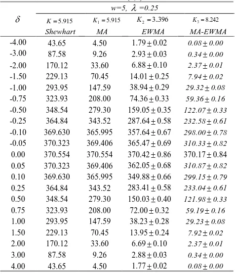
From Table II, Laplace distribution set the parameter

1 0 

 , β

α , MA-EWMA showed that K38.242 (where 25

0 5, λ .

w  ) and ARL₁was lower than MA, EWMA, and Shewhart control charts at all change levels. MA-EWMA control charts had better efficiency in monitoring parameter change than other control chart. If parameter value increased or decreased, _ARL1 resulted showed in Fig 1

From Table III, Logistic distribution set the parameter 2

6 

 , s

μ , MA-EWMA showed that K₃7.632 (where 25

0 5, λ .

w  ) and ARL1was lower than MA, EWMA, and Shewhart control charts at all change levels. MA-EWMA control charts had better efficiency in monitoring parameter change than other control chart. If parameter

TABLEI

ARL PERFORMANCE OF SHEWHART,MA,EWMA, AND MA-EWMA FOR NORMAL(0,1).

 K3.000 K13.000w=5, K=0.25 22.927 K37.632

Shewhart MA EWMA MA-EWMA

-4.00 1.19 1.16 1.080.01 0.000.00

-3.00 2.00 1.62 1.380.01 0.050.00

-2.00 6.30 2.81 2.510.03 0.470.00

-1.50 14.97 3.84 4.190.06 1.510.01

-1.00 43.89 6.97 9.090.15 5.830.02

-0.75 81.22 13.15 16.720.31 13.520.04 -0.50 155.22 35.51 39.930.35 37.180.11 -0.25 281.15 134.51 136.260.48 124.590.35

-0.10 352.93 296.16 307.280.62 243.700.68

-0.05 365.89 348.91 351.090.67 277.220.77

0.00 370.40 370.40 370.000.69 370.050.83 0.05 365.89 348.91 344.660.65 276.830.77

0.10 352.93 296.16 302.150.60 242.740.68

0.25 281.15 134.51 138.840.47 124.390.35

0.50 155.22 35.51 40.760.35 37.200.11 0.75 81.22 13.15 16.700.33 13.520.04 1.00 43.89 6.97 9.110.16 5.870.02

1.50 14.97 3.84 4.180.06 1.530.01

2.00 6.30 2.81 2.540.03 0.470.00

3.00 2.00 1.62 1.390.01 0.050.00

4.00 1.19 1.16 1.080.01 0.000.00

Note that: the italic was minimum of ARL and after the mark

 

 was standard deviation of ARL

ISBN: 978-988-14048-5-5

[image:4.595.311.549.78.355.2]

value increased or decreased, ARL₁resulted showed in Fig 1

From Table IV, the Exponential distribution set the parameter





1

, MA-EWMA showed that K₃4.424

TABLEIII

ARL PERFORMANCE OF SHEWHART,MA,EWMA, AND MA-EWMA FOR LOGISTIC (6,2).

 K17.828 K117.828w=5, K=0.25 23.298 K37.632

Shewhart MA EWMA MA-EWMA

-4.00 123.86 34.42 3.560.03 0.000.02

-3.00 162.83 60.89 8.790.09 0.050.04

-2.00 214.12 110.09 31.520.11 0.470.11

-1.50 245.55 148.75 71.990.25 1.510.20

-1.00 281.59 201.39 153.760.46 5.830.37

-0.75 301.55 234.45 213.530.60 13.520.50

-0.50 322.91 272.99 278.330.71 37.180.65

-0.25 345.78 317.92 338.660.73 124.590.77

-0.10 360.271 348.37 357.460.76 243.700.78

-0.05 365.233 359.15 363.750.78 277.220.79

0.00 370.264 370.26 370.120.81 370.050.83 0.05 365.233 359.15 370.990.80 276.830.79

0.10 360.271 348.37 368.940.79 242.740.78

0.25 345.78 317.92 364.440.78 124.390.77

0.50 322.91 272.99 324.300.72 37.200.65

0.75 301.55 234.45 262.910.62 13.520.50

1.00 281.59 201.39 197.350.48 5.870.37

1.50 245.55 148.75 103.970.24 1.530.20

2.00 214.12 110.09 60.000.13 0.470.11

3.00 162.83 60.89 24.910.11 0.050.04

4.00 123.86 34.42 13.580.09 0.000.02

Note that: the italic was minimum of ARL and after the mark

 

 was standard deviation of ARL

TABLEII

ARL PERFORMANCE OF SHEWHART,MA,EWMA, AND MA-EWMA FOR LAPLACE (0,1).



w=5, =0.25

K5.915 K15.915 K23..396 K38.242

Shewhart MA EWMA MA-EWMA

-4.00 43.65 4.50 1.790.02 0.080.00

-3.00 87.58 9.26 2.930.03 0.340.00

-2.00 170.12 33.60 6.880.10 2.370.01

-1.50 229.13 70.45 14.010.25 7.940.02

-1.00 293.95 147.59 38.940.29 29.320.08

-0.75 323.93 208.00 74.360.33 59.360.16

-0.50 348.54 279.30 159.050.35 122.070.33

-0.25 364.84 343.52 287.640.58 232.580.61

-0.10 369.630 365.995 357.640.67 298.000.78

-0.05 370.323 369.406 365.470.69 310.330.82

0.00 370.554 370.554 370.420.86 370.170.84 0.05 370.323 369.406 362.050.68 310.870.82

0.10 369.630 365.995 349.880.66 299.150.79

0.25 364.84 343.52 283.410.58 233.040.61

0.50 348.54 279.30 150.030.40 121.980.33

0.75 323.93 208.00 72.000.32 59.190.16

1.00 293.95 147.59 38.230.28 29.230.08

1.50 229.13 70.45 13.950.24 7.920.02

2.00 170.12 33.60 6.690.10 2.370.01

3.00 87.58 9.26 2.880.03 0.340.00

4.00 43.65 4.50 1.770.02 0.080.00

Note that: the italic was minimum of ARL and after the mark

 

 was standard deviation of ARL

Vertical lines are optional in tables. Statements that serve as captions for the entire table do not need footnote letters.

a

Gaussian units are the same as cgs emu for magnetostatics; Mx = maxwell, G = gauss, Oe = oersted; Wb = weber, V = volt, s = second, T = tesla, m = meter, A = ampere, J = joule, kg = kilogram, H = henry.

Fig 1. ARL curves of Shewhart, MA, EWMA and MA-EWMA for I) Normal(0,1) distribution; II) Logistic(6,2) distribution; III) Laplace (0,1) distribution; IV) Exponential(1) distribution; and V) Gamma(4,1) distribution.

ISBN: 978-988-14048-5-5

(where w5, λ0.25), and ARL₁was lower than MA, EWMA, and Shewhart control charts at all change levels. MA-EWMA control charts had better efficiency in monitoring parameter change than other control chart,

1

ARLresulted showed in Fig 1

From Table V, Gamma distribution set the parameter 1

4 

 

 , , MA-EWMA showed thatK₃2.0005 ( where w5, λ0.25 _{) and} ARL₁ was lower than MA, EWMA, and Shewhart control charts at all change levels. MA-EWMA control charts had better efficiency in monitoring parameter change than other control chart,

1

ARL resulted showed in Fig 1

V. CONCLUSION

This research purposed the new control chart that was the combination of MA and EWMA control chart called MA-EWMA control chart that studied the MA-MA-EWMA control chart underlying symetrics distribution: Normal(0,1), Laplace(0,1), and Logistic(6,2), and asymmetries distribution, skew to the right Exponential(1), and Gamma(4,1). Findings illustrated that MA-EWMA had better performance than MA, EWMA, and Shewhart charts at all change levels in distributed data Laplace(0,1),

Logistic(6,2), Exponential(1), and Gamma(4,1) but distributed data Normal(0,1) showed that MA-EWMA had better performance than MA, EWMA, and Shewhart chart at all change levels. Only the change at -0.50, 0.50, 0.75 level that the MA chart had lower _ARL1than MA-EWMA chart, however, the value was slightly different. For the research in the future, other distributions may be applied and the other methods to find ARL or other control setting may be added.

ACKNOWLEDGEMENT

The Muban Chombueng Rajabhat University, Thailand and the Graduate College, King Mongkut’s University of Technology, North Bangkok financially supported this paper. The author would like to thank the referees for their valuable suggestions to improve the quality of this paper.

REFERENCES

[1] W. A. Shewhart, Economic Control of Quality of manufactured Product. New York: D. Van Nostrand Company. 1931.

[2] E. S. Page,“Cumulative sum charts,” Techmometrics, vol. 3, no. 1, 1951, pp. 1-9.

[3] S. W. Roberts, “Control chart tests based on geometric moving average, ” Techmometrics, vol. 42, no. 1, 1959, pp. 239-250. [4] D. C. Montgomery, Introduction to Statistical Quality Control. 5th

ed. Hoboken, NJ: John Wiley & Sons, Inc, 2001.

[5] S. W. Butler and J. A. Stefani, “Supervisory Run-to-Run Control of a Polysilicon Gate Etch using in situ Ellipsometry,” IEEE Transactions on Semiconductor Manufacturing, vol. 7, no. 2, 1994, pp.193-201.

[6] M. Khoo, “Poisson moving average versus c chart for nonconformities,” Quality Engineering, vol. 16, 2004a, pp. 525-534. [7] B. C. Khoo and V. H. Wong, “A Double Moving Average Control

Chart,” Communications in Statistics-Simulation and Computation, vol. 37, 2008, pp. 1696-1708.

[8] S. Sukparungsee, and Y. Areepong, “A Study of the Performance of EWMA Chart with Transformed Weibull Observations,” Thailand Statistician, vol. 7, no. 2, 2009, pp. 179-191.

[9] N. Abbas, M. Riaz, and R. J. M. M. Does, “Mixed Exponentially Weighted Moving Average-Cumulatives Sum Charts for Process Monitoring,” Quality and Reliability Engineering International, vol. 29, no. 3, 2012, pp. 345-356.

[10] S. Phantu, S. Sukparungsee, and Y. Areepong, “Explicit Expression of Average Run Length of Moving Average Control Chart for Poisson Integer Valued Autoregressive Model,” in Proceeding of the International MultiConference of Engineers and Computer Scientists 2016, vol. 2, pp. 892-895.

[11] B. Zaman, M. Riaz, N. Abbas, and R. J. M. M. Does, “Mixed Cumulative Sum -Exponentially Weighted Moving Average Control Charts: An Efficient Way of Monitoring Process Location,” Quality and Reliability Engineering International, vol. 31, 2014, pp. 1407-1421.

[12] M. Aslam, W. Gui, N. Khan, and C. Jun, “ Double moving average - EWMA control chart for exponentially distributed quality,” Communications in Statistics, 2017, pp. 1-14.

[13] Y. Areepong, “Explicit formulas of average run length for a moving average control chart for monitoring the number of defective product, ” International Journal of Pure and Applied Mathematics, vol. 80, no. 3, 2012, pp. 331-343.

TABLEIV

ARL PERFORMANCE OF SHEWHART,MA,EWMA, AND MA-EWMA

FOR EXPONENTIAL(1). 

w=5, =0.25

000 . 3



K K13.000 K23.747 K34.424

Shewhart MA EWMA MA-EWMA

0.00 370.55 370.18 370.380.86 370.280.84 0.05 352.482 331.16 263.700.74 228.200.57

0.10 335.291 296.28 192.000.66 160.430.40

0.25 288.59 212.29 85.580.52 67.960.18

0.50 224.75 122.15 33.730.46 25.410.07

0.75 175.04 70.74 19.550.36 13.040.04

1.00 136.32 41.44 13.540.24 8.030.02

1.50 82.68 15.32 7.990.14 4.110.01

2.00 50.15 6.96 5.620.09 2.590.01

3.00 18.45 3.27 3.640.06 1.400.01

4.00 6.79 2.08 2.760.04 0.930.00

Note that: the italic was minimum of ARL and after the mark

 

_ was standard deviation of ARL

TABLEV

ARL PERFORMANCE OF SHEWHART,MA,EWMA, AND MA-EWMA

FOR GAMMA(4,1). 

w=5, =0.25

000 . 3



K K111.786 K23.549 K32.0005

Shewhart MA EWMA MA-EWMA

0.00 370.31 370.03 370.040.87 370.290.84 0.05 342.96 311.96 311.130.80 239.330.63

0.10 317.67 263.29 247.130.67 184.630.49

0.25 252.75 159.46 145.890.45 89.160.24

0.50 173.33 71.27 53.200.34 31.970.09

0.75 119.48 33.63 25.790.33 13.920.04

1.00 82.82 17.22 16.170.27 6.990.02

1.50 40.56 6.52 8.500.10 2.310.01

2.00 20.45 4.07 5.870.06 0.930.00

3.00 5.84 2.30 3.490.03 0.200.00

4.00 2.10 1.53 2.460.02 0.040.00

Note that: the italic was minimum of ARL and after the mark

 

_ was standard deviation of ARL

ISBN: 978-988-14048-5-5