Autaptic circuits for neural vehicles

Autaptic Circuits for Neural Vehicles

Steve Battle

Sysemia Ltd, Bristol & Bath Science Park, Emerson's Green, Bristol BS16 7FR [email protected]

Abstract. This paper develops models for single recurrent neural circuits, known as autapses, where the axon of a neuron forms synapses onto its own dendrites. Once thought to be curiosities or artefacts of growing cells in vitro, autapses play a key role in the operation of Central Pattern Generators and the cortex where they may function as a simple short-term memory. Biologically plausible, idealized models of the autapse are able to produce arrhythmic, sustained behaviours in ‘neural vehicles’. Detailed models are developed to show how excitatory autapses may support both bistability and monostability.

1 INTRODUCTION

The motivation for this work is the development of simple neural circuits for robotic applications. They are biologically inspired, but typically hand-engineered; neuro-engineering rather than neurophysiology. The term Neural Vehicles [9] is inspired by Braitenberg's Vehicles [3]. They are vehicles for understanding neural networks in context rather than as stand-alone circuits. They may be physical hardware robots, software robots, or more abstract vehicles purely for thought experiments. The author uses neural vehicles to teach the principles of artificial neural networks applied to robotics, where they add value as an intuition primer.

Even simple circuits stretch the computational metaphor to its limits, where the aim is not so much as to compute but to control. From the viewpoint of cybernetics, control is as much a first-class citizen as the communication of information. The contention is that robots can teach us a lot about how machines interact with the world around them, both physically and symbolically.

2 BACKGROUND

Aplysia is a genus of large herbivorous sea-slugs found in tropical waters. They are a favourite of neuroscientists because of their small brain, containing just 20,000 neurons, or thereabouts. The Aplysia’s mouth includes a tongue-like rasper (radula) and a cartilaginous structure (odontophore) that enables the mouth to open and close. This mouth structure can be moved in a forward and backward motion (protraction and retraction) that enables it to grasp and tear the plants it is grazing.

Neural circuits that are involved in the generation of motor programs are referred to as Central Pattern Generators (CPGs). The motor programs for protraction and retraction are generated by the Aplysia Buccal ganglia; a Central Pattern Generator for feeding (ingestion and egestion) [16]. The CPG includes a

sub-group responsible for controlling grasper protraction. This sub-group includes neuron B63 and motor neurons B31/B32 that can be triggered by a brief depolarization of B63. Once triggered, their activity is self-sustaining [12]. They are only re-polarized (switched off) by the extrinsic inhibitory action of neuron B64 from an opposing CPG sub-group controlling grasper retraction. The autapse is key to understanding how this persistent electrical and muscular activity may continue long after the initial stimulus has disappeared [1].

3 METHOD

The goal of this work is to describe how simple autaptic circuits can produce the kind of behaviour seen in the Aplysia, and then re-apply this knowledge to the development of simple neural vehicles.

Using standard models of artificial neural networks, and a few carefully selected weights and bias thresholds, it is fairly straightforward to build simple neural circuits that represent combinatorial logic; the operations of conjunction, disjunction and negation. However, the most interesting circuits, and the vast majority of the brain, form recurrent circuits whose behaviour is more difficult to discern. By analogy with electronics circuits we should expect to find circuits with a temporal dimension including differentiators, integrators, oscillators, and bistable & monostable switches. Indeed, the

protraction behaviour of the Aplysia can be understood as the action of a bistable switch [4][8].

3.1 Recurrent Inhibitory Circuits

3.2 Recurrent Excitatory Circuits and the Autapse

However, the space of mutually excitatory neurons is much less well understood and explored. Once thought to be a rarity [2], most cortical connections are local and excitatory. Eighty-five percent of neo-cortical synapses are now thought to be excitatory [5]. The term autapse was first proposed by Van der Loos and Glaser [17]. It is a recurrent connection from a single neuron onto itself, a synaptic connection from its axon onto its own dendritic tree [7]. The study of autapses has traditionally been complicated by the fact that many cells grown in-vitro will readily form autapses that they would not form in vivo. However, numerous studies have confirmed that the brain does grow significant numbers of autapses in vivo. In a quantitative study of the rabbit neocortex, roughly 50% of pyramidal cells were found to contain autapses. More recent studies [15] indicate that the percentage could be even higher [2].

These results may have been overlooked because a simple linear analysis of positive feedback predicts useless runaway behaviours. Like a microphone brought too close to the speaker, a system with positive gain is unstable. However, even in this analogy, the system is not perfectly linear and will saturate at the limits of the amplifier. Neurons are no different; their activation function determines how the input signal, summed within the dendritic tree, is transformed and output. The use of a non-linear saturating activation function completely transforms the dynamics of the positive feedback loop from an impossible infinity into a useful switch.

The concept of the autapse may also serve as a useful simplification to describe larger cell populations. A population of identical neurons with excitatory connection to each other can be simplified to a circuit containing a single neuron with an autapse onto itself [5]. A key feature of such a circuit is the amount of system gain and whether it converges, or diverges until it reaches saturation.

4 RESULTS

The first neuron model comprises a single state variable, x, representing the membrane potential of the neuron; the potential difference between the interior and exterior of the neuron. This determines the firing of the neuron, denoted here by the variable,

y. Rather than representing individual spikes, the activation is averaged over time, such that the output, y, represents the firing rate.

In a simple feed-forward network, the neuron sums inputs arriving simultaneously and will fire at a level that is some function of this input. With a continuous model of neural behaviour, expressed as a differential equation, it is possible to capture the temporal summation of inputs. Neurons perform not only spatial summation of all the inputs arriving along their dendrites, but also temporal integration of inputs that arrive within a short time window [4]. The time span over which this integration can occur is on the order of a few milliseconds (as determined by the membrane time constant). By itself, this mechanism isn't sufficient for integration over longer intervals [6]. Integration over longer timescales can be modelled by a self-excitatory autapse. In this case positive feedback is used to

carry forward output from the previous cycle to be summed into the next.

A biologically plausible neural model will only perform this integration over the timescale of the action potential, or neural spiking. Integration over longer timescales needs a different approach and may be achieved with autaptic circuits [6]. Using positive recurrence, the output reverberates back to the input via the autapse such that when the input stimulus is withdrawn, the neuron continues to be active. Using these ideas, Seung et al [13] describe an autaptic analog memory. This uses positive feedback to create a continuously graded memory but has the drawback that the model needs to be finely tuned so that it is neither converging nor diverging, but is linear and a perfect integrator. If the gain of the system is not exactly 1 then the signal will either leak back to 0, or it will run away to its saturation point.

The bistable model presented here sacrifices analogue fidelity for digital stability. It uses the autapse to perform temporal integration but aims to provide a simple two-state memory rather than one that is continuously graded. The existence of these bistable switches has been observed in the Aplysia, by studying pairs of mutually excitatory abdominal ganglion neurons in vitro [8]. As noted earlier, this small population (of two) may be described as an idealized autapse on a single neuron. This research also emphasizes the extrinsic nature of the inhibitory reset, as opposed to the intrinsic nature of the bistability.

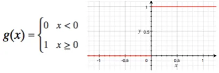
The bistable model presented here does not need to be finely tuned and is tolerant of noise. To achieve this goal, a non-linear activation function is employed. The Heaviside step function is a discontinuous function that is 0 for negative numbers, and 1 for positive numbers. This is a simple 1-bit decision unit that, used in conjunction with a bias value, can test if an input exceeds a given threshold, returning a binary 0 or 1. These Threshold Logic Units (TLUs) are of the style used in McCulloch-Pitts neurons.

Figure 1 - Heaviside step function used to switch the bistable autapse into one of two states

The averaged firing rate, y, is defined in terms of the activation function, g. For simplicity, a simple threshold function is used such that when the potential, x, exceeds the bias the neuron fires. The bias is typically set to a value of 0.5.

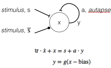
Figure 2 - Bistable autapse defined as an ordinary differential equation. Connections terminating in a bar denote excitatory synapses; filled circles denote inhibition

The autapse is stable in the 'off' position, but when a positive input pushes the potential above the bias threshold, positive feedback amplifies the signal to the point of saturation at which the neuron is fully 'on’. To switch the autapse off again, a negative input is required to push the potential below the threshold at which point it will rapidly decay to 0 and the neuron becomes quiescent in the absence of any further input.

The circuit is not sensitive to the exact nature of the threshold function; a sigmoid function may be substituted for the step function, and works over a wide range of ‘slope’ settings. The circuit is also quite resistant to noise. The simulation of the bistable behaviour in Figure 3 demonstrates how an initial setting of x=0.4 at time t=0 is quickly dampened back to zero. The activation is governed by the saturating linear function that limits the output to the range [0,1]. A system with positive gain and a linear activation function would rapidly amplify small fluctuations through feedback, whereas the non-linear activation function drives the activation level into one of two states. The set and reset stimuli appear as short +/- unit pulses. The activation is self-sustaining because of the excitatory synapse onto itself. The activation level can be seen to be climbing during the pulse and only when it exceeds the bias does the activation level switch ‘on’. An inhibitory stimulus is required to reset the autapse back to the ‘off’ state.

Figure 3 - Plot of the bistable autapse showing the rise in potential in response to the initial positive stimulus, followed

by a self-sustaining activation

The graph illustrated in Figure 3 is generated by the bistable autapse model captured as a Mathematica model in Fragment 1.

This fragment defines the Heaviside step function, g, and the stimulus, s, as a function of time and producing a +/- unit pulse with a given period and duty cycle. Time constants are defined; the time averaging constant, tr=5; the autapse weight, a=1; and threshold bias = 0.5. The simulation is defined to run for 200 seconds.

The activation function is substituted into the differential equation for the neuron, which is then solved for x with an initial value of 0.4 (demonstrating the quashing of insignificant values below the threshold). The results are plotted as in Figure 3, showing the stimulus s, potential x, and activation y.

tr = 5; a = 1; bias = 0.5;

tmax = 200; period = 100; duty = 0.05; g[n_] := If[n <= 0, 0, 1];

s[t_] := UnitBox[Mod[(t-25)/period,1]/(2*duty)] - UnitBox[Mod[(t-75)/period,1]/(2*duty)];

system = NDSolve[{{

x'[t] == (s[t] +a*y[t] -x[t])/tr} /. y[t_] -> g[x[t] - bias],

x[0] == 0.4}, x, {t,0,tmax}]; Plot[Evaluate[

{s[t], x[t], g[x[t]-bias]} /. system], {t, 0, tmax},

PlotRange -> {{0, tmax}, {-1.5, 1.5}}, PlotLegends ->

{"stimulus", "potential", "activation"}, PlotStyle -> Thick]

Fragment 1 - Bistable autapse modeled in Mathematica

This example begs the question as to how to flip the bistable circuit back into the 'off' position. This is treated as an extrinsic inhibitory input. As with the Aplysia, the inhibitory input may come from another CPG.

4.2 Monostability

A further possibility is that there are neural correlates for monostable circuits that are able to reset themselves after a set interval. One plausible mechanism for interval timing is the use of temporal integration in which the firing rate of a neuron gradually increases over time. The end of an interval is marked by the point at which a given threshold is reached [14]. An alternative, single neuron autaptic model that uses signal ramping to reset the circuit can be achieved using internal adaptation to the input. This would allow recurrent excitatory circuits to relax into the 'off' state after a given period of time. The connection strength of the recurrent connection could change, or the threshold could change through adaptation [8].

persistent activity. Translating this into the design of a single neural autapse, this intrinsic adaptation is used to enable the neuron to become adapted to its current state. Furthermore, the rate of this adaptation allows control over the period of time for which the neuron occupies this unstable state. The neural monostable can be thought of as a half-multivibrator.

In the presence of positive recurrence the output must be governed to prevent runaway feedback by setting an upper saturation point. Also, if x goes negative we wish to prevent the autapse from becoming inhibitory. In this case, the activation function g(x) is defined as a saturating linear function of the potential x, limiting the activation to the range [0,1].

Figure 4 - Saturating linear activation function over the averaged membrane potential, x

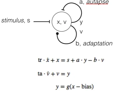
This model extends the basic bistable by adding an additional state variable, v, to represent the current level of adaptation. This varies as a function of the activation, y. This is fed back into the weighted sum for x, via weight a. The rate of adaptation and the resulting interval during which the neuron remains in the unstable state, is determined by ta. The inhibitory reset signal is now intrinsic to the neuron, thus removing the need for an additional source of control.

Figure 5 - Monostable autapse defined as a small system of differential equations. Intrinsic adaptation, v, is shown as

self-inhibition weighted by b

The graph in Figure 6 shows the output of a single monostable autapse with adaptation. A stimulus, s, is required to switch the autapse into the unstable 'on' state. The membrane potential rises, activating the neuron. The activation is self-reinforcing and is sustained even when the stimulus is removed. The activation level remains at the saturation level until the intrinsic adaptation is great enough to inhibit it. It returns to the quiescent ‘off’ state after an interval determined by the rate of adaptation, ta. The time constant for summation of the inputs, tr=3; the time constant for adaptation is an order of magnitude greater and therefore slower, ta=20; The bias is not required so, bias=0; The relative weighting of the excitatory autapse, a=1.7, versus adaptation, b=1, gives more weight to the recurrent input. The simulation is defined to run for 200 seconds. The plot for the activation level is easily recognized by its flat top, at the point where it reaches saturation. Within the range [0,1] it follows the same course as the membrane potential.

Figure 6 - Plot of the monostable autapse showing the response to a momentary stimulus. The inhibitory effect of

adaptation returns the circuit to the stable ‘off’ state

The Mathematica model in Fragment 2 produces the graph seen in Figure 6. It solves the system of two differential equations for the state variables, x and v, after substituting the definition of y. It defines g as a saturating linear activation function with range [0,1], and defines the stimulus, s, as a function of time producing a positive unit pulse of a given period and duty cycle. It plots the stimulus s, potential x, activation y, and weighted adaptation, v.

ta = 20; tr = 3; bias = 0; a = 1.7; b = 1; tmax = 200; period = 100; duty = 0.05 g[n_]:= Which[n<0, 0, n>1, 1, True, n];

s[t_]:= UnitBox[Mod[(t-25)/period, 1]/(2*duty)];

system = NDSolve[{{

x'[t] == (s[t] -b*v[t] +a*y[t] -x[t])/tr, v'[t] == (y[t] -v[t])/ta}

/. y[t_] -> g[x[t] - bias], x[0] == 0.0,

v[0] == 0.1}, {x,v}, {t,0,tmax}]; Plot[Evaluate[

{s[t], x[t], g[x[t]-bias], b*v[t]} /. system], {t, 0, tmax},

PlotRange -> {{0, tmax}, {-0.6, 2}}, PlotLegends -> {"stimulus", "potential", "activation", "adaptation"},

PlotStyle -> Thick]

5 DISCUSSION

In the context of a neural vehicle, the autaptic monostable may be used to realize simple obstacle avoidance behaviour. When a sensor at the front of the vehicle is stimulated, the monostable is triggered, throwing the vehicle into reverse. Like Aplysia, this behaviour must be sustained for a relatively long period of time (a few seconds) to be effective.

The system of differential equations defining each neuron is solved on-board the robot using (forward) Euler’s method. Given initial values for the state variables x and v (typically 0). The step-size is tied to the system clock so the equations are solved in real-time.

Figure 7 - The robot chassis and Arduino based controller serving as a platform for experiments in neural vehicles.

Note the front mounted ‘whiskers’

5.1 Reactive Motor Programs

As discussed earlier, the effectiveness of a neural circuit is best analysed in the context of the system that it controls. To provide a flavour of this approach consider the simple mobile robot in Figure 7. It has two front mounted whiskers that produce a brief pulse when struck. The duration of this pulse is not long enough by itself to drive obstacle avoidance behaviour. However, as we have seen, this stimulus is sufficient to trigger a monostable or bistable switch. It is desirable that the obstacle avoidance behaviour is self-terminating after a short duration so the monostable autapse is the appropriate choice of component.

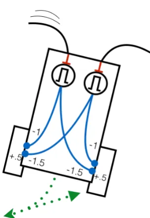
Using the diagrammatic techniques of Braitenberg [3], a simple neural vehicle based on a pair of monostable autapses is illustrated in Figure 8. This style of vehicle uses continuous valued neurons and works with values in the range [-1, +1]. Inhibitory inputs are represented by negative values, and excitatory inputs by positive values. Sensors like the whiskers generate a positive stimulus, while the motors either side of the vehicle can be driven forwards or backwards depending on whether the weighted sum of inputs to the motor (including a bias value, shown) is positive or negative. The autaptic monostable is represented by the circle bearing the monostable symbol (

⎍

Figure 8 - Neural Vehicle with a pair of monostable autapses implementing obstacle avoidance behaviour

When both monostables are in their stable ‘off’ mode, neither motor is inhibited and the (+0.5) bias is sufficient to drive the vehicle forwards. When one of the whiskers is stimulated, the monostable is switched ‘on’. Both motors are inhibited causing the vehicle to reverse. However, the relative weighting causes the motor on the opposite side to run backwards faster, effecting a turn. When the monostable relaxes back to the stable state, the vehicle continues forwards along a straight path, hopefully avoiding the obstacle that triggered the manoeuvre in the first place. Should both whiskers be stimulated, the inhibitory effect on both motors is the same, saturating at -1, causing the vehicle to reverse in a straight line.

5.2 Learning

William Grey Walter, considered by many to be the father of autonomous robotics, saw simple memory devices as a necessary precursor of conditioned learning [18]. In developing his CORA circuit (Conditioned Reflex Analogue) Walter noted the requirement for a short-term memory that could provide a temporal extension of a stimulus. In Pavlov’s classic experiments on the conditioned reflex, the neutral stimulus would be a bell that rings, either simultaneously with, or immediately preceding the specific signal, the presentation of food. For any kind of learning mechanism to associate the two events separated in time, some kind of short-term memory must be present. Once the (extended) neutral and specific stimuli are presented together, their degree of coincidence can be recorded. The monostable autapse provides a biologically plausible mechanism for implementing this stimulus extension.

6 CONCLUSION

Inspired by the biology of Aplysia, this paper has developed simple recurrent neural circuits, autapses, to drive arrhythmic, sustained activities in neural vehicles. Plausible neural models were developed to show how excitatory autapses can support both bistability and monostability (with adaptation). This persistent neural excitation can be understood as a primitive short-term memory that can support simple reactive motor programs or more sophisticated learning.

7 REFERENCES

1. J.M. Bekkers, Synaptic Transmission: Excitatory Autapses Find a Function?, Current Biology, Vol 19, No 7, 2009 2. J.M. Bekkers, Neurophysiology: Are autapses prodigal

synapses?, Current Biology, Volume 8, Issue 2, January 1998 3. V. Braitenberg, Vehicles: Experiments in Synthetic

Psychology, Bradford Books, 1984

4. D. Baxter, E. Cataldo, J. Byrne, Autaptic excitation contributes to bistability and rhythmicity in the neural circuit for feeding in Aplysia, BMC Neuroscience, 11(Suppl 1):P58, 2010

5. R.J. Douglas, C. Koch, M. Mahowald, K.A.C. Martin, H.H. Suarez, Recurrent Excitation in Neocortical Circuits, Science, Vol. 269, 18, August 1995

6. M. Goldman, A. Compte, X. Wang, Neural integrators: recurrent mechanisms and models, New Encyclopedia of Neuroscience, 2007

7. K. Ikeda, J.M. Bekkers, Autapses, Current Biology, Volume 16, Issue 9, 9 May 2006

8. D. Kleinfeld, F. Raccuia-Behling, H.J. Chied, Circuits constructed from identified Apysia neurons exhibit multiple patterns of persistent activity, Biophys. J., vol 57, 697-715, Apr 1990

9. B. Krose, J. Van Dam, Neural Vehicles, in O. OMIDVAR, 271–296, Academic Press, 1997

10. K. Matsuoka, Sustained Oscillations Generated by Mutually Inhibiting Neurons with Adaptation, Biol. Cybern. 52, 367-376, 1985

11. R.F. Reiss, Theory and Simulation of Rhythmic Behaviour due to Reciprocal Inhibition in Small Nerve Nets, AIEE-IRE '62 (Spring) Proceedings of the May 1-3, spring joint computer conference, 171-194, 1962

12. R. Saada, N. Miller, I. Hurwitz, A.J. Susswein, Autaptic Excitation Elicits Persistent Activity and a Plateau Potential in a Neuron of Known Behavioral Function. Current Biology 19, 479–484, March 24, 2009

13. H.S. Seung, D.D. Lee, B.Y. Reis, D.W. Tank, The Autapse: A Simple Illustration of Short-Term Analog Memory Storage by Tuned Synaptic Feedback, Journal of Computational Neuroscience 9, 171–185, 2000

14. P. Simen, F. Balci, L. deSouza, J.D. Cohen, P. Holmes, A Model of Interval Timing by Neural Integration, The Journal of Neuroscience, June 22, 31(25):9238 –9253, 2011 15. G. Tamas, E.H. Buhl, P. Somogyi, Massive Autaptic

Self-Innervation of GABAergic Neurons in Cat Visual Cortex, The Journal of Neuroscience, August 15, 17(16):6352–6364, 1997

16. A. Tiwari, C. Talcott, Analyzing a Discrete Model of Aplysia Central Pattern Generator, Computational Methods in Systems Biology, 6th International Conference, CMSB 2008, Rostock, Germany, October 12-15, 2008

17. H. Van Der Loos H, E.M. Glaser, Autapses in neocortex cerebri: synapses between a pyramidal cell’s axon and its own dendrites. Brain Res, 48:355-360, 1972