Context sensitive optical character recognition using neural networks and hidden Markov models

Rochester Institute of Technology

RIT Scholar Works

Theses

Thesis/Dissertation Collections

1992

Context sensitive optical character recognition

using neural networks and hidden Markov models

Steven C. Elliott

Follow this and additional works at:

http://scholarworks.rit.edu/theses

This Thesis is brought to you for free and open access by the Thesis/Dissertation Collections at RIT Scholar Works. It has been accepted for inclusion in Theses by an authorized administrator of RIT Scholar Works. For more information, please contactritscholarworks@rit.edu.

Recommended Citation

Rochester Institute of Technology

Computer Science Department

Context Sensitive Optical Character Recognition

.

uSIng

Neural Networks and Hidden Markov Models

by

Steven C. Elliott

A thesis, submitted to

The Faculty of the Computer Science Department in partial

fulfillment of the requirements for the degree of

Master of Science in Computer Science

Approved by:

Professor P. G. Anderson

Professor R. T. Gayvert

Professor

J. A. Biles

PERMISSION GRANTED

Title:

Context Sensitive Optical Character Recognition using Neural Networks and

Hidden Markov Models

I STEVEN C.

ELLIOTT

hereby

grant permission

to the Wallace Memorial Library of

the Rochester Institute of Technology to reproduce my thesis

in

whole or

in

part. Any

reproduction will not be for commercial use or profit

ABSTRACT

This

thesis

investigates

a method

for

_using contextual

information

in

text

recognition.

This is based

on the premise

that,

while _reading,

humans

recognize words with

missing

or garbled characters

by

_examining the

surrounding

characters and then

selecting

the appropriate character.

The

correct character

is

chosen

based

on an

inherent knowledge

ofthe

language

and

spelling techniques.

We

can then modelthis statistically.

The

approach taken

by

this

Thesis is

to combine

feature

extraction

techniques,

Neural Networks

and

Hidden

Markov Modeling. This

method of

character recognition

involves

a three _step process: pixel

image

preprocessing,neural network classification and context

interpretation.

Pixel image

preprocessing

applies a

feature

extraction algorithm to

original

bit

mapped

images,

which produces a

feature

vector

for

the original

images

which are

input

into

a neural network.

The

neural network performs the

initial

classification ofthe characters

by

producing ten weights, one

for

each character.

The

magnitude of the

weight

is

translated

into

the confidence the network

has

in

each of the choices.

The

greater the magnitude and _{separation, the} more confident the neural network

is

of a given choice.

The

output ofthe neural network

is

the

input for

a context

interpreter.

The

context

interpreter

uses

Hidden Markov

Modeling

(HMM)

techniques to

determine

the most probable classification

for

all characters

based

on the

characters that precede that character and character pair statistics.

The

HMMs

are

built

_using an a priori

knowledge

ofthe

language:

a statistical

description

oftheprobabilities of

digrams.

Experimentation

and verification of this method combines the

development

and use of a preprocessor _program, a

Cascade Correlation

Neural Network

and a

HMM

context

interpreter

program.

Results

from

these experiments show the neural network _successfully

classified

88.2

percent ofthe characters.

Expanding

this to the word

level,

63

TABLE OF CONTENTS

1.0

Introduction

1

2.0

Artificial Language Generation

6

3.0

Project Description

3.1

Feature Extraction (Image

Preprocessor)

9

3.2

Neural Network Models

14

3.2.1

Hopfield

Network

14

3.2.2 Back

Propagation Network

16

3.2.3

Cascade Correlation

20

3.3

Context

Interpreter

(Hidden

Markov

Modelling)

26

4.0

Results

and

Conclusions

33

4.1

Feature

Extraction

Results

33

4.2

Neural Network Results

34

4.3

Hidden Markov Model Results

38

4.4

Conclusion

41

5.0

Recommendations

for Future

Research

42

6.0

Bibliography

43

7.0

Appendices

A

Handwritten

Digit Examples

B

List

of

Words

in

Vocabulary

C

Neural

Net Output

(Observation

Probabilities)

LIST OF FIGURES

Figure

1

Pattern

to

Object Relationships

2

Figure

2

System Architecture

5

Figure 3

Initial Probabilities

6

Figure

4

Transition Probabilities

7

Figure

5

Sub-Feature

Graphic

10

Figure

6

Pixel

Map

Sub-Windows

11

Figure

7

Feature Matrices

12

Figure

8

Hopfield

Network

Architecture

14

Figure

9

2

Layer Perceptron

Architecture

16

Figure

10

Cascade Correlation Architecture

23

Figure

11

Hidden

Markov

Model

Terms

28

Figure

12

Viterbi Algorithm

29

Figure

13

Actual Transition Probabilities

31

Figure

14

Network Results for Individuals

35

Figure

15

Network

Confusion

Matrix

36

[image:6.552.100.460.129.419.2]

1.0

Introduction

This

thesis

investigates

a method

for

_using contextual

information in

text recognition.

This is based

on the premise

that,

while _reading,

humans

can use context to

help

identify

words garbled

by

_misspelling,

bad

penmanship,

bad

printing

etc.,

by

examining

the surroundingcharacters and

then

selecting the

_{appropriate character.}

The

correct character

is

chosen

based

on

familiarity

of _the

language

and _{spelling techniques.}

The

reader

routinely

uses

knowledge

about the syntactic, semantic and

featural

dependencies between

characters and

between

words

[1]

.

The

use of

knowledge

about

dependencies between

characters within

words

is

explored

in

this

Thesis.

The

method we use

in

this

Thesis

does

not

explore the

dependencies between

words

but

our method could _easily

be

expandedto

include

"global context".

This

paper proposes a method

for

pattern recognition combined with

the

knowledge

ofthe character context _{to successfully}

interpret handwritten

digits

combined as words.

Two

aspects of this recognition process are

investigated:

the recognition ofthe

individual

patterns

(characters)

and the

combination ofthepatterns

into

specific words.

Pattern

recognition

has

traditionally

been

grouped

into

two general

categories: the "statistical" or "decision theoretic"

approach and the

"structural/syntactic"

approach

[2].

The

statistical or

decision

theoretic

approach

is

often referred to as a geometric approach.

This

_methodology

focuses

on

how

a pattern

is

constructed and

how

that pattern maps to the

objectthat

it

represents.

Within

the geometric _approach, patterns are

described

by

their

components, which can

be

viewed as vectors

in

a coordinate space of

N

dimensions.

Each

pattern then corresponds to a point

in

that space.

With

this type of _{representation,}

familiar

mathematics

become

available

for

pattern recognition.

Euclidean

distances between

two points

become

a

similarity metric

for

characters.

Two

patterns that represent similar or

identical

objects would

be

expected to

be

very close to each other

in

pattern

space;

however

it is

usually necessary to replace thepixel arrays with

feature

vectors.

The

_relationship

between

the geometric

description

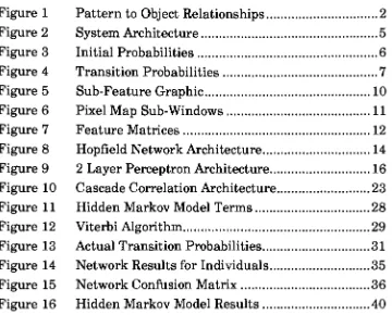
of a pattern and

on one ofthree classifications.

The

relationship

between

a pattern and the

object

is

deterministic

if

there

is

a one _{to one,} or a _{many to} one _relationship

between

the

pattern or patterns and the object

being

represented.

A

non-deterministic

relationship

exists

if

a pattern can represent more than one

object

(or

class).

The

non-deterministic _relationship

is

probabilistic

if

different

probabilities can

be

attached

to

the various relationships.

A

representation

is

stochastic

if

there

is

a

finite

_{probability that} an object can

be

represented

by

points anywhere

in

thepattern space.

These

relationships

are shown

graphically

in

Figure

1.

Deterministic

Non-Deterministic

Stochastic

Figure

1

In

character recognition of machine printed

text,

if

_onlya single

font is

used, and the system

is

_completely

free

of_{noise, then} each pixel _array would

map to a single object.

A

deterministic

geometric representation would

be

realized.

If

multiple

fonts

were _used, multiple pixel arrays would represent the same object

(i.e.,

different

version of the

letter

"A").

In

_{this case,} a

deterministic

representation

is

also realized.

In

the case of recognition of [image:8.552.109.471.223.543.2]

different

objects

(such

as the confusion

between

the characters

"I",

"1" and

"1").

This

results

in

the generation of non-deterministic relationships.

If

finite

probabilities can

be

assigned to each case then the relationship

is

said

to

be

stochastic.

In

the

case where non-deterministic or stochastic relationships exist,

additional

intelligence

must

be built into

the system

to

differentiate between

similar patterns.

The

use of

this

intelligence is

referred to as context

directed

pattern recognition

[3].

Context directed

pattern recognition can

be

either syntactic or stochastic

in

nature.

To

use the syntax ofa

language for

pattern _recognition, weneed to

have

theproduction rules which were used to

generate the

language.

This

approach

has been

taken with the use of

Augmented Transition Networks (ATN).

Using

_{this method,} characters are

represented as nodes.

The

transition,

or _arc,

from

one node to another can

only

be

completed

if

the conditions

imposed

on those arcs

have been

meet.

One

major

difficulty

associated with the use ofthis type of context

in

pattern

recognition

is

determining

how

the grammar

is

to

be

inferred.

The

stochastic approach to context

directed

pattern recognition

is

not

based

ontheproduction rulesthatgeneratethe

language,

but

rather

is

based

on the statistical_make-up ofthe

language. This

approach usesthe statistics

which

indicate

what characters occur and what order those characters occur.

This

statistical

knowledge

ofthe

language

can

be

obtained

from

the

language

without

knowing

_any of the syntax or production rules that were used to

generatethe

language.

The

use of

Hidden Markov

Models

best describes

this

typeof context

directed

patternrecognition.

For

this

Thesis,

we

developed

an artificial

language

which consisted of

100

_words, each

5

characters

in

length.

The

characters

for

thewords are the

digits

0

thru

9.

These

digits

were each

handwritten,

scanned and then

digitized. The

statistical characteristics ofthe

language

was

determined

and

used as part ofthepatternrecognition process.

The

approach taken

by

this

Thesis

was to combine three separate

recognition techniques

into

a single _{system, utilizing the}

benefits from

each

technique.

These

three techniques were:

feature

_extraction, neural networks

and Hidden

Markov Modeling.

The feature

extraction process

looked

within

characters as words _and,

based

on

its

knowledge

ofthe

language,

helped

to

resolve

the

correctword classification.

The

feature

extractionalgorithm examined the original pixel maps

for

features

corresponding

toevidence

for lines

(strokes)

at various places

in

four

orientations

in

the

image.

The

output of

the

feature

extraction algorithm was a

feature

vector representativeoftheoriginal

image.

The feature

vectors were used as

input into

aneuralnetwork.

The

neural network wasused toperformthe

initial

classificationofthe

characters.

The

training

data for

the neural network consisted of

half

ofthe

handwritten

character

database,

while the second

half

of the

database

was used

for

testing

purposes.

The

neural network selected the

digit

most _closely

identified

by

the

feature

vector.

The

neural network

had

ten output _nodes, each output node represented a specific

digit.

The

magnitude of the output value was translated

into

the confidence ofthe neural network

for

that classification.

The

greater_{the magnitude, the}greaterthe confidence.

These

confidences

for

each classification were recorded

for

use

in

the next_step ofthe process.

The

output of the neural network was then used

by

the context

interpreter.

The

context

interpreter

used

Hidden

Markov

Modeling

techniques to

determine

the most probable classification

for

all characters.

The HMMs

were

built

_using an a priori

knowledge

of the

language

-a

language

model.

The

model

included

the

initial

state probabilities

(the

probability a

digit

was the

first digit

of a word) and the transition probabilities

for

a specific

digit

to

follow

another

digit

within the word

(digram

statistics).

The

context

interpreter

examines the probabilities of all

of the characters within word

boundaries.

The

output of the

HMM

was a sequence of

digits

that

best

correspond to the

input

ofobserved

digits.

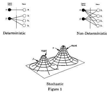
System Architecture

Database of

1200 Handwritten

Digits

Feature Extraction

Feature

Vector

Database

Feature

Vector

Database

Training

Data

Testing

Data

Neural

Network

Classifications & Observation

Probabilities

Vocabulary

Hidden Markov Model

Final

[image:11.552.75.479.149.551.2]

Word Recognition

2.0

Artificial Language Generation

Input

into

the

system was

from

a

database,

supplied

by

Bell

Laboratories

[4],

consisting

of

1200

handwritten digits.

The database

was generated

by

having

12

individuals

write

the

set of

digits (0

thru

9)

ten times.

Each

set of

digits

₀

_through

9,

for

_each

individual

was considered an

attempt.

Each

digit

was

labeled

according to

who wrote

it

and

during

which attempt

the

digit

was created.

The

attempts were

labeled

"A" through "J".

This

resulted

in

120

distinguishable

attempts of the

10

digit

set.

These

sampleswere then scanned and normalized

into

1200

separate

16

by

16

pixel maps.

The

maps were then converted

into

an

ASCII

readable

format.

Within

_{the maps,} a "#" character represents a

logical

1

(black

_pixel), while the " "

(space)

characterrepresents a

logical 0

(white

pixel).

Examples

ofthe

handwritten digits

andthenormalized pixel maps are shown

in

Appendix

A.

These digits

provided the

basis for

the generation of the artificial

language. The language

_vocabularyconsisted of

100

_words, each word was

5

digits

in

length.

The language

was generated

by

first

_selecting an

initial

character probability.

This

determined

the

first digit

for

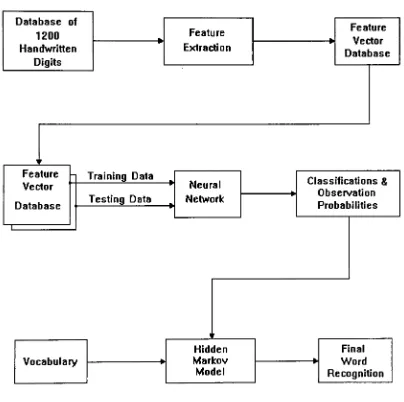
each word.

The

initial

_{probabilities,} shown

in

Figure

3,

were chosenat random.

Digit

Initial

Probability

0

.05

1

.20

2 .05

3

.05

4 .00

5

.10

6

.25

7

.04

8

.01

9

.25 [image:12.552.167.384.412.658.2]

In

additionto

the

initial

probabilities,

the transitionprobabilities were

selected.

This information indicated

with what _probability one

digit

would

follow

another

digit

within a word.

This

only

applies within words and

does

not cross word

boundaries.

For

example,

a "2" will

follow

a"1" ten percent of

the

time,

while a "1" will

follow

a "2"

only

five

percent ofthe time.

These

values were chosen

arbitrarily in

order to provide some type of selection

process.

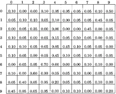
The

transition

probabilitiesare shown

in

Figure

4.

The

digits down

the

left

side are the

first

of a _pair, while the

digits

across the

top

are the second.

0

1

2

3

4

5

6

7

8

9

0

0.10

0.00

0.00

0.10

0.05

0.05

0.05

0.05

0.10

0.50

1

0.05

0.10

0.10

0.05

0.10

0.00

0.05

0.05

0.45

0.05

2

0.00

0.05

0.35

0.00

0.00

0.00

0.00

0.45

0.00

0.05

3

0.10

0.05

0.00

0.05

0.15

0.05

0.50

0.05

0.00

0.05

4

0.10

0.10

0.05

0.05

0.05

0.45

0.10

0.05

0.05

0.00

5

0.10

0.05

0.00

0.05

0.45

0.10

0.05

0.10

0.05

0.05

6

0.00

0.05

0.05

0.70

0.00

0.00

0.00

0.10

0.10

0.00

7

0.10

0.00

0.60

0.00

0.05

0.05

0.10

0.00

0.05

0.05

8

0.05

0.40

0.05

0.05

0.20

0.05

0.05

0.05

0.10

0.00

9

0.45

0.05

0.05

0.05

0.00

0.10

0.10

0.00

0.00

0.20

Figure

4 -

Transition

Probabilities

A

program was written to use the

data from Figure

3

and

Figure

4

to

generate theartificial

language.

This language is

shown

in

Appendix

B.

The data from

Figure 3

and

Figure

4

was also used

for

the

Hidden

Markov

Modeling,

this

is

discussed

in

section

3.3.

The database

of

handwritten digits

was used to generate the words [image:13.552.74.456.240.550.2]

the neural network, while attempts

F

thru

J

were used

for

testing

of the neural network and

the

context

interpreter.

All

of the

digits

in

all of the attemptswerepassed through

the

feature

extraction algorithm.

3.0

Project

Description

3.1

Feature

Extraction

Sub-System

The

first

process within the recognition system

is

the

feature

extraction sub-system.

Feature

extraction allows

for

statistical character

recognition.

With

this

_{method, the} classification of the patterns was

based

on selected

features

which

have been

extracted

from

the original pixel _map, rather than

template matching

of the pixel maps themselves.

This

makes the system more

tolerant

of minor variations

[5].

Pixel

_{map matching} would

be

effective

if

the

distortions

were of the

"salt

and pepper noise" type.

Handwritten

characters

have

"plastic

distortion".

The

difficulty

with

feature

extraction

is

knowing

what

features

to extract and

how

those

features

should

be

represented.

The

selection ofthese

features

was

largely

empirical and ad

hoc,

and

drew

upon our

knowledge

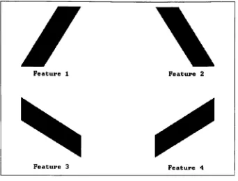
of the problem.

Four

primitive

features

were selected

for

extraction

from

the original patterns.

All

of the

features

were

lines,

each with

different

slopes.

These

features,

known

as

Convolution Kernels for

Feature

Extraction,

are shown

in

Figure

5.

These features

were

implemented

because

of their simplicity.

Additional

features

such as

line

intersection,

horizontal

lines,

etc. could

be

implemented

aspart of_any

future

research project.

The

feature

extraction algorithm maps the original pixel _array

from

feature

space to

decision

space.

From

the

decision

_space, the output vectors

were mapped to the appropriate objects.

Classification

of the pattern was then

based

on theoutput

feature

vector ratherthan the pixel map.

The feature

extractionalgorithmused

here

is

similar_{to convolutions,}a signal _processing technique.

Convolutions

are common and powerful techniques

for

filtering

images.

A

convolution

is

a _specially

designed filter

(matrix)

that

is

combined together with a portion of an

image

to compute a transformed pixel value.

The

filter,

or convolution

kernel,

is

centered on each pixel

in

the

initial

pixel map.

The

sum ofthe product ofthe

filter

and the underlying

image

is

computed.

The

result

is

a transformed value of the

center pixel.

The

filter is

then moved to the next pixel and the process

is

repeated.

Some

special _{processing may}

be

needed to take

into

account

the

Feature 1 Feature 2

[image:16.552.104.446.73.333.2]

Feature 3 Feature 4

Figure 5

The

convolution ofthe

filter

and

image is

determined

by

_{computing the}

point to point product of _{the corresponding} elements of the

filter

and the

portion of the

image

which

is

being

_overlaid, and then _{summing those}

products.

By

properly selecting

kernels for

a

filter,

the convolutions can

detect

lines,

edges, create

high

and

low

pass

filters,

and _variety of other

functions

[6].

The feature

extraction algorithm presented

here

applies

four

filters

to

the original pixel

image.

The

four

filters

represent the

four

features

which

are

being

extracted

from

the original

image.

Each

filter

is

designed

to

determine

if

the

feature

it

represents

is

present

in

_{the underlying} portion of

the pixel map.

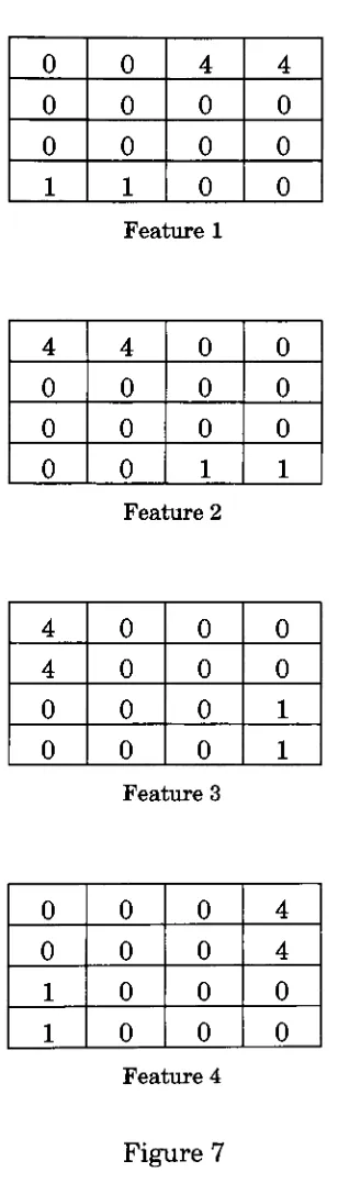
Each filter

is

represented

by

a

4

by

4 matrix, whose values

are

designed

to

detect

the

desired

features.

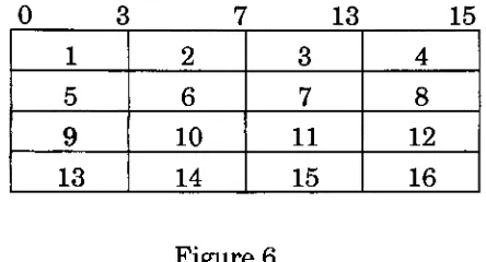
The

original pixel maps were

divided

into

sixteen

4

by

4

pixel areas as

shown

in Figure 6.

The

four

feature filters

are applied to each area.

Each

filter is

overlaid overthe

designated

area.

The

pairwise products ofthe

filter

greater than

4

but

not

divisible

by

4,

then

the

feature is

present, otherwise

the

feature is

notpresent.

All

sixteen areas of original pixel

map

were overlaid with the

four

feature filters

to provide a

feature

vector made _up of

64

elements.

Each

element represents

the

presence ofa specific

feature (or

evidence ofa stroke) within a specific area.

The

elements of

the

output

feature

vector are

binary

values, with a

1

indicating

the

presenceofthe

feature

and a

0

indicating

that the

feature

wasnot present.

0

3

7

13

15

1

2

3

4

5

6

7

8

9

10

11 12

13

14

15

16

Figure

6

Each

primitive

feature

was confined to the

4

by

4 _window; that

is,

no

features

crossed windows or wrapped around at the edges.

Unlike

the

image

processing convolutions, the

filters do

not center on a single pixel

but

examinethe entire area ofthe

filter.

The

filters

are moved

from

area to area

(4

pixel row

increments),

in

the order shown

in Figure

6,

instead

of_moving

from

pixel to pixel.

No

_mirroringof pixels was performed attheedges.

Using

this

technique,

a

16

by

16

pixel _map

(256

elements) was represented

by

a

64

bit

_vector, thus providing a

4

to 1 compression ratio.

This

compression was convenient

for

use of the

feature

vector as

input

into

theneural network.

[image:17.552.162.384.222.342.2]

0

0

4

4

0

0

0

0

0

0

0

0

1

1

0

0

Feature 1

4

4

0

0

0

0

0

0

0

0

0

0

0

0

1 1

Feature 2

4

0

0

0

4

0

0

0

0

0

0

1

0

0

0

1

Feature 3

0

0

0

4

0

0

0

4

1

0

0

0

1

0

0

0

[image:18.552.201.355.94.632.2]

Feature 4

Each

of the

overlay

filters

were applied

to

all of the quadrants.

The

general notation

for

this

calculation shown_symbolically

is:

3 3

Q

=

Z Z

WijFij

i=o j=o J

J

where:

i,

j

= _{relative row and column coordinates}

W

= _{window area of original pixel}

map

F

= convolution

kernel

Q

= summationof pairwise product

The

value

Q

wasthentested to

determine

if

theparticular

feature

was present.

lifQ>4ANDQ*8)

Vk

=

0

otherwise

Where

Vfc

is

the

kth

component ofthe

feature

vector.

3.2

Neural Network Classification

Artificial

neural networks

have

been

_widely used

in

pattern

recognition applications.

Various

paradigms

have been

used.

The

different

networkmodels are specified

by:

1.

Network

topology:

the

number ofneuronsand

how

theneurons

are

interconnected.

2.

Node

characteristics:

the

typeof non-lineartransfer

function

used

by

theneuron

for

calculating

theoutput value.

3.

Training

rules: _specify

how

theweights are

initially

set and

adjusted to

improve

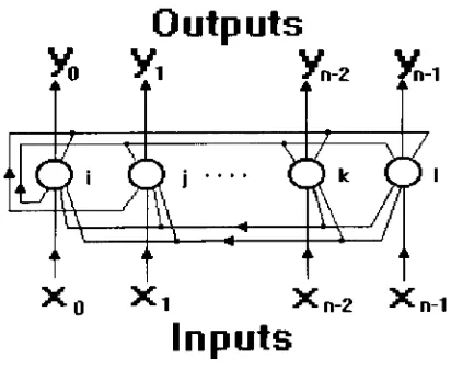
performance ofthenetwork.

3.2.1

Hopfield

Network

One

such paradigm

is

the

Hopfield

network

[7]. The Hopfield

network

is

a

hand

programmed associative memory.

It

is

composed of a _single,

fully

recurrent

layer

ofneurons that act as

both input

and output.

The diagram

of a

Hopfield

network

is

shown

in

Figure

8.

Outputs

X)

Yl

Xn-2

Xi-1

X0

Xt

Xn-2

Xn-1

Inputs

Figure

8

The

output ofthe neurons

is

passed

back

as

input

_{to the neurons, thus} [image:20.552.191.397.423.592.2]

connected,

i.e.,

for

all

i

and

j,

Wjj

=

Wji?

and

Wy

=

0

,where

Wy

is

the synaptic weight

connecting

neurons

i

and

j. The

neurons are updated

by

therule

Xj

=

fllWijXi)

(Eq.

1)

where

Xj

is

the

output of neuron

i.

The

function f is

generally

non-linear;

such as _{signum, tanh}orthesigmoid_y =

(1

₊ e"x)_1

The

non-linear

function

compresses the output so that

it lies

in the

range

between

0

and

1

or

between

-1 and +1.

This is

sometimes referred to asthe

squashing

function.

The Hopfield

network

does

not

learn

through execution ofthe net.

The

weights must

be

set

in

advance.

The

weight matrix

is

created

by

taking

the outer product of each

input

pattern vector with

itself,

and _summingall ofthe outer_products, and

setting

the

diagonal

to

0.

The Hopfield

network can complete or restore corrupted patterns

by

matchingnew

inputs

with the closest _previously stored patterns.

The

input

pattern vector

is

applied to the network node.

The

network then cycles through

iterations

until

it

has

converged.

Convergence

is

when the outputs of the network no

longer

change on successive

iterations.

Hopfield

proved thatconvergence

is

alwaysguaranteed.

The

Hopfield

network

has

two major

disadvantages.

The

first

is

the number of patterns thatcan

be

stored.

It has

been

shownthat the maximum number of patterns recalled

is

_generally

limited

by

_{n/(21og n),} where n

is

the numberof nodes

[8]

.

3.2.2

Back Propagation Network

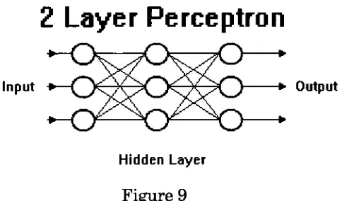
The back

propagation model or multi-layer perceptron

is

a neural network

that

utilizes a supervised

learning

technique.

Typically

there are one or more

layers

of

hidden

nodes

between

the

input

and output nodes.

See

Figure

9.

The

multiple

layers

allow

for

thecreation of complex contours

defining

decision

regions.

A

single

layer

perceptron can _only create a

half

plane

bounded

by

a

hyperplane decision

region.

A

two

layer (single hidden layer

between input

and output) perceptron _easilyallows

for

the creation of convex

decision

regions, while a three

layer

(multiple

hidden

layers)

perceptron allows

for

the creation of _arbitrarily complex regions

limited

by

the number of

hidden

nodes.

More

difficult

to see

is

_{that any}

decision

boundary

can

be

achieved with a

2

layer

_network,

but

this can

be

_very complex.

2 Layer

Perceptron

Input >

f

_/C

X

JXXL

)0()

? Output [image:22.552.187.429.337.479.2]

Hidden Layer

Figure 9

The

use ofthe

back

propagation

training

algorithm requires the use of a non-linear,

differentiable

transfer

function

within each node.

The

sigmoidal

function described

above

fills

these requirements.

The back

propagation

training

algorithm

is

a supervised

learning

technique.

Input

vectors are matched withthe

desired

output vectors.

These

pairs are referred to as the

training

pairs.

The

network

is

trained using a

To

train a multi-layer perceptron _using

back

propagation, the general algorithm

is

as

follows:

1.

Set

the

initial

starting

synapticweights tosmall random

values.

2.

Apply

the

input

vector

from

the

training

pairto the network.

3.

Propagated

the

vectorthrough thenetwork

using

thenon

linear

transfer

function

tocalculate theoutput of

the

network.

The

calculations are performedon a

layer

by

layer

basis.

4.

Calculate

theerror_value, which

is

thesquared

difference

between

the

actual output andthe

desired

output vector

from

the

training

pair.

5.

Propagate

theerror signal

back

_{through the output,}

hidden

andto the

input layers

adjusting

theweightsto minimizethe

error.

6.

Iterate

steps

2

through

5

for

all ofthe

training

pairs within

the

training

set until theerror

level for

theentireset

is

acceptably

low.

In

more specific

terms,

the neurons are

initialized

to the

input

values.

The

states of all other neurons

(xj)

in

the network are

determined by:

Xj

=

flZWijXi)

(Eq. 2)

The

nonlinear

function

f

needs to

be

differentiable,

so we use tanh or the

sigmoid:

y

=

(l+e-X)-l

(Eq.3)

This

calculation

is done

layer

by

layer

with the output of each

layer

serving as

input

into

the next

layer.

This

continues until the nodes on the

output

(rightmost)

layer have been

computed.

The

error

E

ofthenetwork

is:

E

=

Z(Xk

- tk)2

Where

the

sum

is

over

the

output _nodes,

Xfc,

whose "target" output

is

t^

(from

the

training

data).

Training

consistsof

determining:

AWij

=

-a

(6E/6Wij)

(Eq.

5)

where a >

0 is

the

training

rate

for

one pass

(epoch)

over

the

training

data.

First

we adjust

the

weights of

the

output

layer. The back

propagation

algorithm uses a

technique

similar to

the

"Delta

Rule"

developed for

perceptrons.

The

"Delta

Rule"

is

shown as:

where:

Wy(n+1)

=

Wij(n)

₊

AWy

(Eq.6)

tfc

=_{target output}

X^

=

Actual

_output

8

=_{error signal}

AWjj

= _correction

corresponding

to the

ith

input %i

a =

learning

_{ratecoefficient}

Wjj(n+1)

=_{value oftheweight afterthe adjustment}

Wjj(n)

= _{value of}the_weight

before

_{theadjustment}

The back

propagation algorithm uses the

derivative

ofthenon-linear

squashing

function f().

If

y =

(1

_{+e~x)"l, then}

y'

=

y(l-y)

(Eq.

7)

Which

makes the calculation _particularly easy.

No

new

function

needs to

be

evaluated.

The

use ofthe partial

first derivative

ofthe error

function

allows

for

a

simple gradient

decent

search technique

in

finding

the global minima

for

the

error value.

Training

the output

layer

of the network

is

fairly

straightforward

The

following

equations show the

training

process

for

determining

a single

weight

between

neuron

(p)

in hidden layer

(j)

_{to output neuron}

(q)

in

_the output

layer

of

the

network:

5q

=

yqd

-yq)(t

-yq)

(Eq.

8)

AWpq

=

r|

oq

yp

(Eq<

9)

Wpq

(n+1)

=

Wpq

(n)

+

AWpq

(Eq.

10)

where:

t =

target

_output

for

_neuron

q

yq

=

Actual

_{output of neuron}

q

8q

= _{error signal}

for

_neuron

q

A[

= _correction

corresponding

to the

ith

input

Xi

r\

=

learning

rate coefficient

Wi(n+1)

=_{value ofthe weight afterthe adjustment}

Wj(n)

=value ofthe weight

before

the adjustment

The

_adjusting of the weights of the

hidden

layer

is

more

difficult

because

the

desired

output ofthese neurons

is

not

known.

Back

propagation trains the

hidden

layer

by

_{propagating the} output error

back

through the

network, adjusting theweights at each

layer.

The

error value

(5)

must

be

calculated without

knowing

what the

desired

output of the

hidden layer

neurons should

be.

The

error value

8 is

first

calculated

for

each ofthe output

layer

neurons.

These

error values are then propagated through the associated

input

weights

(of

the output

layer

neuron)

back

to the

first

hidden layer

neuron.

These

propagated error values arethen usedto adjust the

input

synaptic weights

for

the

hidden layer. The

same procedure

is

used again to propagate the error value

back

to the next

hidden layer

ortothe

input

layer.

The

error values calculated

for

theoutput

layer

(Eq.

8)

is

multiplied

by

the weightthat connects the output neuron with the

hidden

neuron.

This is

done for

all the connections

between

the output

layer

and the

hidden layer

summing

all of the products and then _multiplying that value

by

the

derivative

of

the

non-linear sigmoid

function (Eq.

7).

Calculating

the new

weight values

is

same

for

the

hidden layers

as

it is for

the output

layers

as

shown

in

equations

(Eq. 9

and

Eq.

10).

The

equation

for

determining

the

hidden layer

error value

is

as

follows:

6P

j

=

^p

jd-yp

j)

(5q,kWpq>k)

(Eq.

11)

While

the

back

propagation network

is

much

improved

over the

Hopfield Network for

pattern _{recognition, there} are still caveats with the

algorithm thatmust

be

overcome.

The

most severe

limitation is

the

length

of

time required to train a network.

For

complex _{problems, the}

training

time

could

be

_excessive, or even more_{serious, the} network_may

fail

and _maynever

be

trained.

The

network

training

failures

are_usuallyattributedto one oftwo

sources: networkparalysis or

local

minima.

Network

paralysis occurs whenthe synaptic weights

become

_very

large

values.

This

forces

the output ofthe neuron to

be large.

This is

in

a region

where the

derivative

ofthe non-linear sigmoid

function

would

be

_very small.

The

smaller this value, the slower the

training

becomes,

until the

training

appears to

be

at avirtual standstill.

The

Back Propagation

uses gradient

decent

to

determine

theminimum

error value

for

a neuron.

The

error surface of a complex network _may

be

filled

with _many

hills

and valleys.

Local

minima occur when the network

settles

in

a shallow _valley when there

is

a much

deeper

_valley

(global

minima) nearby.

There

is

_generally no _way of

knowing,

without time

consuming experimentation, what

is

the right network architecture

for

a

given problem.

3.2.3

Cascade

Correlation

In

an attempt to overcome the

limitations

mentioned above

for

the

back

propagation

learning

_algorithm, the

Cascade

Correlation

network

times

was examined.

The

Cascade Correlation

network paradigm was used

for

this

Thesis.

Two

major problems were

discovered

which contribute to slowness of

the

back

propagation

learning

algorithm.

The first

problem

is

the

"step

size"

problem and

the

second

is

the

"moving

target"

problem.

Several

clever

strategies were

incorporated

in the

Cascade Correlation

algorithm which

helped

speed

up

the

training

times.

A

network

learns

when

the

error value

for

each neuron

is

reduced to

an acceptable

level.

The Back Propagation

algorithm uses a partial

first

derivative (Eq.

7)

ofthe error values with respectto the weights to perform a

gradient

decent

in

weight space.

The

rate that this

decent is

made

is

related to the

step

size.

If

infinitesimally

small steps are

taken,

_{then calculating the}

error values after each _step will _eventually result

in

_obtaining a

local

minimum of the error

function.

While

_{this may work, the time to} perform

each ofthe

training

steps could

be

infinitely

long.

If

the steps taken are too

large,

the

local

minimum _may never

be

reached

because

the

large

_step might

not provide the resolution needed to

find

the

local

minimum.

If

a

local

minimum

is

_reached,

it

has been

_empirically

determined

that the

local

minimum will

be

theglobal_minimum, or at

least

a "goodenough solution"

for

most problems

[10].

In

orderto choose an appropriate_{step size,} additional

information

(not

part of the original

Back

Propagation

algorithm)

is

needed.

In

addition to the slope ofthe error

function,

information

about

its higher

order

derivatives

or curvature

in

_{the vicinity}ofthecurrent _point,can

be

used.

The

_quickprop algorithm

[11]

estimates the second order

derivative

of

the error

function

to update the synaptic weights and

determine

the

local

minimum.

For

use ofthe quickprop _algorithm, two simplifying assumptions

were made:

1.

Small

changes

in

one weight

have

little

or no effect onthe error

gradient seen at other weights.

2. The

error as a

function

ofone synaptic weight can

be

approximated

by

a parabola _openingupward.

As

part of the algorithm, the

first derivative

calculated

for

the previous

last

made to each weight.

Using

the

previous slope value, the current slope

value and the

last

weight _change, a parabola can

be fit

to those points and

the

minimum pointoftheparabolacan

be determined

analytically.

The

procedure

for

the quickprop

algorithm

is

_{essentially the} same as

the steps

for

the

Back Propagation

algorithm.

The

major

difference is

the

calculation used to

determine

theweight update value.

The

equation used

in

the

quickprop

algorithm

is

shown

symbolically

as:

AW(t)

=

(S(t)

/

S(t-l)

-S(t))

AW(t-l)

(Eq.

12)

where:

S(t)

= _{current error}

derivative

S(t-i)

= _{previous error}

derivative

AW(t-i)

= _{previous weight change}

The

second problem

identified

as a source of slow

learning

with

Back

Propagation

is

referred to as the

"moving

target"

problem.

Each

neuron within the

hidden layers

ofthe network are

feature detectors.

The

learning

process

for

these

layers

is

complicated

by

the

fact

that all the other neurons

are also _changing at the same time.

Each

neuron within the

hidden

layers

only see

its

own

inputs

and the error signal propagated

back

to

it from

the next

layers.

The

error signal that the

hidden

neuron

is

_{attempting to}

focus

in

on

is

_{constantly changing,} therefore causing the

hidden

neurons to take a

long

time tosettle

in

and

determine

the

desired

local

minima.

One

ofthe

difficulties

with multi-layer perceptrons

is

determining

the

number of

hidden

neuronswithin thenetwork.

The

number of neurons must

be large

enough to

be

able to

form

a

decision

region that

is

suitable

for

the

given problem.

Caution

must

be

taken not to

have

too many neurons so that

the number of weights required cannot

be

estimated

from

the available

training

data.

Prior

to

Cascade

Correlation,

theexperimenter

had

to

fully

_{specify the}

network architecture

before

the

training

began.

It

was not

known

if

the

Cascade Correlation

combines two

key

elements to

help

solve the

"moving

target"

problem.

The first

element

is

the cascade architecture.

Using

thecascade

architecture,

hidden

neurons are added tothe network one

at a time as

the

network

is

training.

Once

a neuron

has been

_added,

its

input

synaptic weights are

frozen,

and

only

the weights associated with

its

outputto theneuronconnectedto

the

next

layer

are adjusted.

The

second element addedwas an attemptto maximizethe magnitude

ofthecorrelation

between

thenew neuron's output and theerror signal

being

eliminated.

As

new

hidden

neurons are _added, each new neuron receives a

connection

from

all ofthe network's original

inputs

and also

from

all ofthe

previously added

hidden

neurons.

This

is

a change

from

previous

architectures

in

which the neurons of one

layer

were _only connected to the

neurons ofthe next

layer.

The input

synaptic weights are

frozen

when the

new unit

is

added.

An

example ofthe

Cascade

architecture with two

hidden

nodes

is

shown

in Figure 10

2nd Hidden

Unit

Q_

1st Hidden_/~N

Unit

C)

Input

+-Output

[image:29.552.193.394.367.518.2]

66

Figure 10

The

network

begins

with no

hidden

neurons.

The

network

is

trained

using the quickprop algorithm until the error value reaches a minimum.

If

this value

is

acceptable, the

training

is

complete.

If

the error value

is

not

acceptable, a new unit

is

added,

its

input

weights are

frozen

and the output

connection weights are then trained using the quickprop algorithm.

The

process continues again until the

training

is

acceptable, or another unit

is

To

add anew_{neuron, the} system

begins

with apool of candidate units.

Each

of

the

candidate neurons are

initialized

with a

different

set of random

input

weights.

All

of

these

neurons receive

input from

all of

the

network's

initial inputs

as well as

from

all ofthe

existing

hidden

neurons.

The

outputs

of

these

neurons are notyet connected to the

remaining

network.

A

number

ofpassesover

the

training

data is

used toadjust the

input

weights.

The

goal

is

to maximize

the

magnitude of the correlation

between

the new neurons

output and the residual error signal.

This

correlation

(actually

_co-variance)

is:

where:

S

=

2

I

X

(Vp

-V)

(EP)0

-E')

I

(Eq.

13)

o= networkoutput at which error signal

is

measured

p=

training

_pattern

V

=_{candidateneuron output value}

E0

= residual output error observed at neuron o

V

=_{value of}

V

_averaged

for

_all

input

_patterns E'

=_{value of}

E0

averaged

for

all

input

patterns

The

correlation value

S

is

maximized _{using the quickprop}

training

algorithm.

When

the

training

is

complete

for

the pool of candidate neurons

(patience is

exhausted), theneuron with the

largest

correlationto the error

is

inserted

into

thenetwork.

The

use of the candidate pool _greatly reduces the risk of

installing

a

neuron that was "untrainable".

It

allows the system to

try

_many

different

areas

in

weightspaceto

find

agood solution.

The

network architecture used

for

this

Thesis

was

Cascade

Correlation.

The

system

had

64

input

neurons with

10

output neurons.

The

64

input

neurons correspond to the

feature

vector extracted

from

the original

pixel maps.

A

major purpose ofthe

feature

extraction algorithm was

data

compression.

If

the

feature

extraction

had

not

been

_{run, the}

input layer

of

the network would

have had

256

neurons.

The

10

output neurons correspond to the ten

digits

0

through

9.

have

one of the output neurons equal to +0.5 and the remaining

9

output

neurons equal

to

-0.5.

The database

of

1200

handwritten digits

was

divided into

two separate

sets.

The first

set of

600

was used

for

training

of_{the network; the} second set

of

600

digits

was used

for

testing.

The

original

database

contained ten

attempts

by

twelve

individuals

to write the ten

digits.

The database

was

split such that each set

(training

and

testing)

contained

5

attempts

by

all

twelve

individuals

at_{writing the ten}

digits.

The

training

of the network required

345

epochs.

An

epoch

is

one

complete passthrough the

training

data.

Upon

_completion, when there were

zero _{errors, the}

Cascade Correlation

algorithm added_only

2

hidden

neurons.

Once

thenetwork was

trained,

the test

data

was used as

input

into

the network.

For

each

input

_vector, the output of the network was recorded.

This

included

what

input

pattern was presented to the _network, the

classification ofthe vector

by

thenetwork and the output value

for

all ofthe

output neurons.

This

information

was

kept for

use

in

the next stage ofthe

system, thecontext

interpreter,

_utilizing

Hidden

Markov Modeling.

The

network was able _{to correctly classify}

529

of the

600

test

file

patterns

for

a success rate of

88.2

percent.

Specific details

describing

the

3.3

Context Interpreter (Hidden Markov

Modeling)

The

third

and

final

stage of oursystem

is

the

context

interpreter.

This

stage uses a

knowledge

about

the

dependencies between

the characters

within the words to

help

determine

the correct classification of the words.

This

stage

is

added

to the

output ofthe neural network classifier

because

to

date,

neural networks are notwell suited

for

dealing

with time varying

input

patterns and segmentationof sequential

inputs [12].

The

technique

for

modeling

the context ofthe words

is

Hidden Markov

Modeling

(HMM).

This is

a statistical approach

for

_modeling an observed

sequence ofpatterns.

This is

in

contrast to other models that utilize syntax

and semanticstomodelthe context ofthe

desired

patterns.

Hidden

Markov

Modeling

techniques

have been

used

for

speech

recognition problems

for

numerous years.

There

are _strong similarities

between

speech recognition and character _recognition, which makes the use

of

Hidden

Markov Models

a

logical

choice

for

optical character recognition.

A

Hidden

Markov

Model

is

a

doubly

stochastic process with an

underlyingstochastic processthat

is

not

directly

observable

(hidden),

but

can

only

be

observedthrough another set ofstochastic processes thatproduce the

sequence of observed symbols

[13].

The HMM

is

a collection of states with

interconnecting

transition arcs.

Associated

with each state

is

an observation probability.

This

is

the

probabilityof

being

in

_anygiven state at _anygiventime.

Associated

with the

transition arcs are transition probabilities.

These

define

the probabilities of

moving

from

one statetoanother.

In

terms of optical character _recognition, the observation probabilities

are

defined

as the probabilities that a specific object

is

represented

by

the

given

input

pattern.

The higher

the _probability, the more certain the

recognition process

for

thatparticularpattern.

The

transition probabilities are

defined

as the probabilities of

having

one character

follow

another character within the word.

For

_example,

in

English,

there

is

a

higher

_{probability that the} character "U" will

follow

the

character "Q" than the probability that the character

"Z"

will

follow

the

character"Q".

This

type of_modelingcan_easily

be

expanded to provide global _context,

Depending

on the system

being

_{modeled, the}

"a

priori"

knowledge

that

is

required

is

sometimes

difficult

to

obtain.

For

this

Thesis,

a single

HMM

was created and utilized.

This

model

represented the entire

language.

The

transition probabilities were

based

on

all of

the

words

in

the

language.

An

alternative approach would

have been

to create a model

for

each _{word, then test the vocabulary} against _every

model.

The

model that produces the

best

results

is

interpreted

as the model

of the word

being

recognized.

This

approach _commonly used

in

speech

recognition.

Describing

and _using

HMMs

requires the

definition

of the

formal

symbolic terms.

These

are shown

in

Figure

11.

Also

shown,

in

parenthesis,

are the

descriptions

of

how

these elements were

defined for

character word

recognition.

The

variables

A,

B

andII are themost _critical, so

for

_compactness, the

HMM

(X)

is

represented as a

function

ofthose threevariables:

X

=

(A, B,

n)

When

_using

HMMs

to evaluate and model a specific

domain,

three

problems must

be

solved

for

the model to

be

useful.

These

problems are

evaluation,

decoding

and training.

The first

problem, evaluation, states

that,

given a model and a

sequence of _{observations,} calculate the _probability that the observed

sequence was produced

by

themodel.

The

most straightforward approach to _{solving this} problem

is

the

"brute force" method.

This

method calculates the _probability

for

every

possible state sequence of

length

T.

This

procedure _quickly

becomes

unfeasible as the number of states

(N)

increases

and the

length

of the

observation sequence

(T)

increases.

The

number of calculations required to

determine

the_probability

is

(2T

-1 )NTmultiplicationsandNT-1 additions.

In

response to this problem, the

forward-backward

algorithm was

developed

[14].

With

this procedure, the probability of partial observations

up to a given state are calculated

from

the

beginning

of the model.

Also

calculated

is

the probability of a partial observation

back

to a given state

starting at the output of the model and _working

back.

These

two

probabilities are summed.

The

number of calculations required

for

this

T

=

length

ofobservation sequence

(

numberof

digits in

each word

)

N

=numberofstates

(

numberof

different

digits

available

)

M

=_{number of observation sequences}

(

number ofoutput

digits

)

Q

=

{Qi>

Q2> >

Qd

individual

states

(

individual digits

)

V

=

{v^,

. . _., vm}

discrete

set of possible

symbol_occurrences;

(

set of

digits

0

through

9

)

A

=

{a^ay,

_{statetransition probability}

(

probabilityone

digit

following

another

digit

)

B

=

|bj(k)},

bj(k),

_observation

probability

distribution

in

state

j;

(

_probabilityof an

input

vector_representingeach specific

digit)

n

=

{t^},

_7ti5

initial

state

distribution

(

probabilityof each

digit

being

the

first

digit

of a word

)

Figure

11

The

second _problem,

decoding,

states that given a sequence of

observations, what was the optimal path through the model

(state

_sequence)

that produced the observation.

This

uncovers the

hidden

portions of the

model.

The Viterbi

algorithm was

developed

to solve the

decoding

problem [image:34.552.99.464.58.526.2]

Viterbi

Algorithm

1.

Initialization

-Set initial

state values

5i(i)

=

nibi(01),

1

_<;

i

_^

N

^(i)

=

0

2.

Recursion

Maximize

state sequence

For2^t^T,

l<ij^N

8t(j)

=_{max[8t.1(l)Aij]Bi(Ot)for 1<}

i

_<

N

Yt(j)

= _{argmaxtS^DAy]}

forl^i^N

3.

Termination

-

All

states

have been

traversed

P*

= _max[8T(i)]

for

1 _<l

i

_<:

N

i*T

= _{argmax[8T(i)]}

for

1_^

i

_<

N

4.

Backtrack

-

Determine

optimal state sequence

For

t =

T

-1,

T-2,

. . . _, 1

Figure

12

The

algorithm

finds

the optimal state sequence

for

the observation

sequence.

To determine

the optimal state _{sequence, the} most

likely

state

is

determined

at each

instance in

time

(t).

The

_probability

is

based

on _the

probability of

being

in

the previous state

(W(tl)(i)),

the transition

probability

from

theprevious state to thecurrent state and the observation

probability

of

the symbol

in

thecurrent state.

This

_value,

(Vt(i)),

is

then maximized

for

all [image:35.552.95.463.52.529.2]

the

Viterbi

algorithm well suited

for

dealing

with recognition and

segmentation.

The Viterbi

algorithm was used

for

this

paper to select

the

best

sequenceofstates

for

theobserved sequences.

The

net result ofthis

function

was

the

optimal state sequence.

The

sequencewas

interpreted

asthe context

directed

recognized word.

The

state sequence corrected mis-classified

digits

based

onthecontext

knowledge

ofthe artificial

language.

The

_{third problem,}

training,

examines

how

to optimize the parameters

ofthe

HMM

so to maximize the

probability

of a given observation sequence.

This

allows

for

the

adjustment ofthe

HMM

to

best

suit the

domain.

This is

the most

difficult

problem _{relating to the}

HMMs.

There is

no

way to solve this problem analytically.

The Baum-Welch

algorithm was

developed

as an

iterative

technique

[16]. The

threevariables

(it,

A

and

B)

are

re-estimated, then evaluated.

If

_{the probability} ofthe observation sequence

increases,

then the new values are saved.

The

algorithm guarantees that

either the probability

improves

or a critical point

had

_already

been

reached

wherethe probability

had

_already

been

maximized.

In

_{creating the}

HMM

for

this application, the

initial

probabilities

(n)

used were the same probabilities used to generate the vocabulary.

These

probabilities are shown

in

Figure

3.

The

transition probabilities

(A),

were

determined

by

examining the vocabulary.

The

transition probabilities are

shown

in

Figure

13.

These

are _slightly

different

than the transition

probabilities used to generate the

language (see

Figure

4)

because

of

0

1

2

3

4

5

6

7

8

9

0

1

2

3

4

5

6

7

8

9

0.122

0.00

0.00

0.122

0.073

0.073

0.073

0.073

0.122

0.341

0.047

0.116

0.116

0.047

0.116

0.023

0.047

0.047

0.419

0.023

0.000

0.059

0.353

0.00

0.00

0.00

0.00

0.500

0.029

0.059

0.082

0.082

0.000

0.061

0.143

0.061

0.449

0.061

0.00

0.061

0.154

0.115

0.038

0.038

0.077

0.423

0.115

0.000

0.038

0.000

0.094

0.062

0.031

0.062

0.312

0.156

0.062

0.094

0.062

0.062

0.000

0.034

0.034

0.661

0.017

0.000

0.000

0.119

0.119

0.017

0.094

0.000

0.469

0.000

0.094

0.062

0.125

0.031

0.062

0.062

0.032

0.355

0.032

0.032

0.194

0.032

0.032

0.097

0.129

0.065

0.434

0.038

0.038

0.019

0.000

0.113

0.151

0.000

0.00

0.208

Figure

13

The

observation probabilities

(B)

used

for

the model were generated

from

the neural network.

The

output values

from

each output neuron were

recorded

for

_every

input

vector.

The

output values were thennormalized and

used asthe observationprobabilities.

A different

set of observation probabilities were used

for

each person's

attempt

in

_{writing the}