INTRODUCTION
The productivity modeling is a commotion used to ascertain the important contributions and yields of a certain manufacturing process. It guesstimates the steady state performance at op-timum working settings and shape process model parameter crosswise the operational range [1]. This commotion involves three process stages. The Screening Stage: in which all conceivable noteworthy inputs and outputs of the process are identified and further conducting a sequence of running certain experiments so as to minimize any tilt to these process inputs and outputs [2]. These experiments help to develop preliminary process model for studying the relationships be-tween the process variables. The Mapping Stage: here the performance of the key factors over their predictable working ranges is mapped through a sequence of more exhaustive experiments [3]. The Passive Step: during this stage the process is al-lowed to run at minimal working conditions for estimating the process reliability and fitness[4]. Process enhancement is an important fragment
of any unremitting development program for the persistence to examining the physical fitness of the running process [5]. Apparently all the manu-facturing and measurement practices display pro-cess variation. Though the propro-cess variability is an amassing of various sources of variation that have arisen through the production process, the critical actions of process are to recognize and enumerate these foundations of variation so that they may be diminished and improve the process [6]. There are two such types of process variations. Controlled variation: Variation which is considered stable and present a reliable design of variation over time, however such type of variation is normally ran-dom which will present a uniform variation about a continuous level [7]. Uncontrolled variation: a variation that fluctuates over time that is why it is unpredictable, however such type of variation normally contains some edifice [8].
Outlines of the process model
The first step is to develop the model with desired parameters under study for validation
Volume 13, Issue 2, June 2019, pages 157–167
https://doi.org/10.12913/22998624/106240
Statistical Analyses of Productivity Model Parameters
for Process Improvement
Zahid Hussain
11 Sarhad University of Science and Information Technology, Peshawar 25000, Pakistan e-mail: [email protected]
ABSTRACT
Productivity modeling and validation is the assessment of data to establish scientific indications that a process is
stable. The aim of this paper is to present a novel approach using statistical analyses for process improvement.
This study highlights the process behavior of three different lathe machines unit with the intention to replace one of them. The research methodology has illustrated by producing a steel rod of 3.175 millimeter diameter based on 180 samples collected from each machine. For statistical data value analysis, MS Excel 2016 and Minitab 18 were utilized. The results showed that lathe machine 1 and 2 had an equivalent inconsistency, but significantly different
data spreads. Similarly, the throughput for machine 2 was higher with greater variability as compared to machine
1 while machine 3 encountered a low rate of throughput. On the basis of the fallouts of the analysis, the research team has officially suggested to substitute lathe machine 3.
Keywords: statistical analyses, process modeling, experimental design, process improvement.
Research Journal
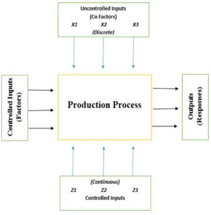
Accepted: 2019.05.05[9]. In this perspective a black box model as shown in Figure 1 is motivated by necessary input variables which may either be controlled or uncontrolled and presented as process fac-tors and responses correspondingly. The inputs perform some process changes and produce the required outputs. These outputs usually present some specific of the process and usually mea -surable [10]. Further, they could be sampled in order to perceive and apprehend how they actu-ally perform and relay to each other. The process factors and responses are pigeonholed rendering to variable type that demonstrates the expense of evidence they cover [11].
Experimental design considerations
For the process reliability and capability, it is normally intended to distinguish between the interactions among the factors and responses. During conducting the current study, two types of responses relationships are addressed [12].
Correlation: when an experimental change of a single process variable is supplemented by a change of another one. Causality: when there exists a causal relationship between the two pro-cess variables in case a variation in the range of one process variable brings a variation in the other one respectively[13].Usually, during ex -perimental investigation, it is intended to deter-mine correlation and confirm causal interactions using various techniques in order to manipulate experimental data [14].
Productivity parameters considerations The principal action of the productivity pa-rameters considerations for building modeling and validation is to gather the required data in order to present conclusions for the maximum and effective improvement [15]. The steps in -volve are presented in Figure 2. The furthermost significant step considerably is the planning that should engender like a declaration of the goals, expressive process validation model, explana-tion of the sampling, depicexplana-tion of the data col-lection technique, jobs with errands, configur -ing, and putting away a sketch of the process data analysis [16]. All those verdicts that distress the significance of the process characterization will likely be directed throughout the planning stage. The process parameters should be di-rected according to the plan supported with all omissions renowned [17]. Data collection is fun-damentally the implementation of the sampling strategy. It is based on the fact that if a good task were completed during the planning phase, then the current step becomes much more straight-forward. It is significant to complete the plan as strictly as conceivable and to highlight any ex-emptions [18]. Data analysis and explanation is the mishmash of quantifiable statistical analysis practices similar to ANOVA, regression and cor -relation followed by graphical techniques that exhibit scatter plot, histograms and box plots which are practical to the data collection for the accomplishment of the process parameters [19]. Reporting is also a critical step which should not be disregarded. In order to create a revealing re-port, it must be ensured that others concerned
Fig. 1. Process black box
have the chance to open access to the material made by the production [20]. The main impartial of this paper is to plan and develop productivity modeling for a real industrial process validation with the help of engineering statistical methods. Practical work has been conducted in a com-pany’s mechanical workshop where three lathe machines are engaged to produce the desired product. This research work will also extend a group of engineering statistical approaches to put on the experimental models into actual in-dustrial conditions scientifically that involve the study and development of the process improve-ment rate [21].
MODEL ASSUMPTIONS
Primarily, it is assumed that the process may sufficiently be modeled as the total of a methodi -cal and random constituent. The methodi-cal con-stituent is the mathematical model portion while the random constituent is the noise or errors ex-isting in the process system [22]. It may also be assumed that the methodical constituent is stable over the level of working environments while the random constituent has a continuous position, distribution and spread arrangement [23]. Lastly, the data collection measuring strategy has been deliberated and confirmed to the anticipated ex -actness and correctness.
Continuous linear production model
The continuous linear production model is based on numerical function that transmits de-scriptive process variables to a solitary continu-ous response process variable that is:
(1)
The expression explains that if there exist any p explanatory process variables, then the required response is demonstrated through a constant time and over a total of functions of the process explan-atory variables with some expected error [24].
One-way ANOVA
A one-way outline involves a single process factor with numerous levels and manifold annota-tions at each considerable level while the outline computes the mean of the annotations inside each level factor. However, the residuals will explain the dissimilarity within each process level [25]. By doing so the nonconformity of the mean of individual level of the grand mean is analyzed to recognize roughly about the unusual effects. Similarly, the variation is compared within differ -ent levels to the dissimilarity across levels using the expression 2 that specifies that any jth value, from a specific level i, is the total of basically three constituents that is the grand mean followed by the deviation of separately level mean from the grand mean and the residual [26].
yij = m + ai + eij (2)
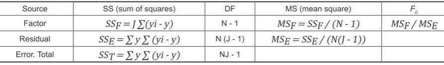
Approximation for the one-way arrangement may be performed by calculating the total vari-ance, within level followed by the across level variance and could be summarized using ANOVA table as shown in Table 1 to recognize any signifi -cance pertains to factor levels.
Here:
(3)
And
(4)
Using expression 3 and 4 with ANOVA, test -ing is conducted to find that the observed process data for any significant variance between their means [27]. If it is further assumed that the data observations within each factor level hold the same variance, then the variance of each factor level is calculated and mere these observations together to study the estimate of the overall pro-cess data variance [28]. It can be exposed that the specified assumptions regarding the process data, the ratio between the level of the mean square
Table 1. ANOVA table for analysis
Source SS (sum of squares) DF MS (mean square) F0
Factor SSF = J ∑(yi - y) N - 1 MSF = SSF / (N - 1) MSF / MSE
and the mean square of residuals follows the F distribution with specified degree of freedom as presented in one-way ANOVA table. However, if the value of F0 is significant at any significance level, then it will clearly show that there is defi -nitely a level upshot existing in the data [29]. As -sumption: For the purpose of estimation, it is as -sumed that the process data can be successfully modeled as the total of a deterministic element and a random constituent. It is further assumed that the stable constituent may be modeled as the total of the overall data mean with extra influence from the level of factors [30]. It is finally assumed that the random elements are desired to be mod-eled with the Gaussian distribution approach with a stable data spread and location [31].
METHODOLOGY AND DATA COLLECTION
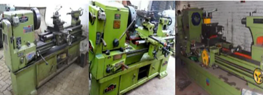
Current study emphasizes the prominence and relevance of engineering statistical approach to analyze three different lathe machines installed in Frontier ceramic industry in Peshawar city with the commitment to replace one of them. This work basically focuses on data collection, inves-tigation and implication using statistical analysis approaches. For data values comparison, the state of the art statistical software package Minitab 18 is utilized so that evocative glitches could be highlighted. These machines are installed in me-chanical workshop and are in the state of normal working conditions as shown in Figure 3.
At present the industrial unit has sufficient potential to substitute one of the machines. In this regards the research and development depart-ment of the unit had been assigned to carry out
a practical a study and make an endorsement as to which specific lathe machine could be substi -tuted. It was also decided to observe one of the utmost regularly parts produced, a steel rod of 3.175 millimeter on each of the machines and to observe which particular lathe machine is the slightest stable. The data collection process starts with performing statistical analyses containing ascertaining and working with various probabil-ity distributions followed by vigilant planning strategy. Planning is the most important step that comprises of the description of strong and brief goals, developing process sensitivity model and formulating a sampling plan.
Outlining the goals
The primary goal of this research study is to explore which specific machine is basically least constant to produce the required steel rod of de -sired size with a tolerance of ± 0.003 millime -ter respectively. For measurement of the process stability, a continuous variance around a mean will be considered and in case when all of the three lathe machines are observed to be stable, then the judgement will likely be based on the process inconsistency and throughput. Finally, the machine with the maximum variability and lowest productivity output will be designated for possible replacement.
Sensitivity modeling
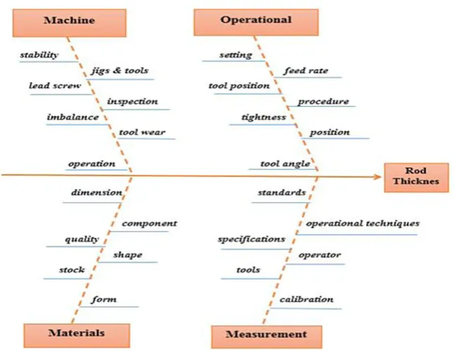
The purpose of sensitivity modeling is to model the relationships of the identified process factors and responses by selecting a parameter and ascertain the other parameters which might have
an effect on it. This task is simply documented with a Fishbone diagram as shown in Figure 4. All the three machines will collect bar stock from the similar spot. There is a slight difference in ma -chine, hence the concerned operator should make alterations to the rotation of the part, feed rate at which the screw is made with desired cut and stop to each machine. It is also noticeable that the same machine operator will run all machines at the same time. Measurement is also important, hence an ex-perience inspecting engineer is assigned to collect the produced samples and record the necessary measurements. Finally, the consideration of the lathe machine physical condition which is the real aim of the current research work. The reliability of the machining process will mostly be determined by the wear on the guideways and the lead.
Sampling plan
After confirming the productivity modeling and goal declaration, the next step is to delineate the sampling plan. Here the principal objective is to define if the given process is unstable and to associate the discrepancies of the process with machines. It is also desirable to observe each ma-chine’s throughput in order to portray and com-pare the required productivity of these machines. For this purpose, a three day run time of the actual sampling was scheduled to study and examine the consequences based on statistical analyses. To do
this a suitable time of the day is considered that did not affect the normal industrial activities. It is occasionally the situation when the lathe ma-chines are almost idle, especially at the start of the morning shift at 9.00 and at the end of the shift at 17.00 respectively. Hence the decision is to pro -duce samples at these available times. In order to avoid any other industrial activity conflict too ruth -lessly, it was therefore acknowledged to sample only 10 pieces, two times a day, for three consecu -tive days from each individual machine while the daily based throughput of all three machines will be exercised accordingly. The samples produced
Fig. 4. Fishbone diagram for potential parameters identifications
and collected are shown in Figure 5 respectively. Finally, the corresponding throughput of the parts encountered from each machine would be calcu-lated at the end of each consecutive day.
DATA ANALYSIS AND RESEARCH
FINDINGS
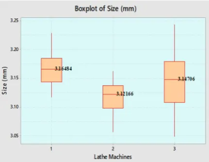
As soon as the relevant machines data have been collected from the maintenance engineering department of the industrial unit, the required data analysis process variables were tabulated in a stake format as shown in Table 2. The next stride is to accomplish a quality status and check the data set in order to confirm normality. Figure 6 represents a fitted line of the normal distribution that signi -fying that sample data contributes an excellent and precise theoretical distribution, whereas the solid curve of the data histogram to the frequen -cies bars demonstrate that the distribution of the data is almost normal while the process stability estimations are seems to be consistent for the cur-rent production process. During the next phase, it is intended to explore which certain factors have an influence on which specific process response variability and to measure its significant influence. In this regards, it is appropriate to compare the outcomes by plotting box plots of the measured data of each machine with respect to the size of the specimen in the millimeter that is the explana-tory process variance. Such comparison is shown in Figure 7 representing the box plot of the size (mm) with respect to lathe machines. It has been
revealed from the observations of the box plots that the location of data median looks to be sig-nificantly different for the three lathe machines in which the second machine showing the lowest av-erage size of 3.1216 millimeter. On the other hand, machine 1 has the output of the highest average size of 3.1645 millimeter respectively. It is also noticeable that both machines 1 and 2 have some-what an equivalent inconsistency, however lathe machine 3 has a considerable greater variability.
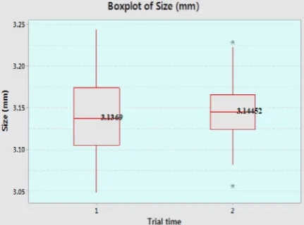
Figure 8 presents the box plot of the specimen size with respect to the Run and it may also be observed from the box plots analyses that neither the data location nor the data spread look to differ significantly. On the basis of Figure 8 findings, the box plots presentation shows that the trial time with respect to the specimen size clearly shows
Fig. 6. Probability and histogram estimates of the data samples and process stability
that neither the data location nor the data spread seem to differ significantly by trail time of day. However, observing the findings revealed from Figure 9, which shows the box plot of the speci
-men with respect to size, it may be concluded that even though there are some slight differences in data location and extent between the specimen, these alterations do not demonstrate a perceptible outline and do not look significant.
Therefore, the clarification of the box plots may be established by conducting analysis of variance using equation 1 to 4 for the four fac -tors related to lathe machines, Run, Trial time and specimen while the outcomes of ANOVA are in -corporated into Table 3. The output of ANOVA is interpreted to establish the required production process characterization model and the using ex-pression 5 to fit the model.
yij = μ + αi + βi + γi + φi + eij (5)
The analysis will lead to develop the regres-sion equation for the estimations of the effect as contrasting to the model, therefore equation 6 is introduced to establish the process of fitting a conscious function to the data set points.
Table 2. Experimental data of the process variables
Observation Lathe machine Run Trial time Specimen Size (mm)
1 1 1 9.00 1 3.1623
2 1 1 9.00 2 3.2054
3 1 1 9.00 3 3.1750
4 1 1 9.00 4 3.1775
5 1 1 9.00 5 3.2029
6 1 1 9.00 6 3.1724
7 1 1 9.00 7 3.1800
8 1 1 9.00 8 3.1419
9 1 1 9.00 9 3.1318
10 1 1 9.00 10 3.1877
… … … … … …
180 3 3 17.00 10 3.1699
Fig. 8. Box plots comparison of trial time
yij = ai + bi + ci + di + eij (6) The following regression equation is obtained on the basis of expression 5 and 6 that models the process variables and to predict values within the range of the data set which clearly specifies that only
the factor pertains to machine is observed to be statistically significant.
Size (mm) = 3.14332 + 0.02376 Lathe Machine_1 - 0.02530 Lathe Machine_2 + 0.00154 Lathe Machine_3 + 0.00357 Run_1 + 0.00192 Run_2 - 0.00549 Run_3 - 0.00258 Trial time_1 + 0.00258 Trial time_2 - 0.00614 Specimen_1 + 0.00261 Specimen_2 - 0.00092 Specimen_3 - 0.00346 Specimen_4 + 0.00797 Specimen_5 - 0.00388 Specimen_6 + 0.00275 Specimen_7 - 0.00515 Specimen_8 - 0.00487 Specimen_9 + 0.01107 Specimen_10
Preceding analysis of variance specified that a single machine factor was statistically significant, however the Table 4 shows the ANOVA outcomes used for lathe machine factor only. Particularly in this phase, it is the point of interest to analyze levels of means for the lathe machines variable which is summarized in Table 5 respectively.
Table 3. Summary of ANOVA for four factors
Source DF Adj SS Adj MS F-Value P-Value
LatheMachine 2 0.072416 0.036208 29.90 0.000
Run 2 0.002794 0.001397 1.15 0.318
Trial time 1 0.001196 0.001196 0.99 0.322
Specimen 9 0.005691 0.000632 0.52 0.857
Error 165 0.199819 0.001211
Lack-of-Fit 164 0.197106 0.001202 0.44 0.865
Pure Error 1 0.002713 0.002713
Total 179 0.282236
Table 4. Summary of ANOVA for machine factor
Source DF Adj SS Adj MS F-Value P-Value
Lathe Machine 2 0.07267 0.036337 30.69 0.000
Error 177 0.20956 0.001184
Total 179 0.28224
In order to validate the production pro-cess characterization model, it is nepro-cessary to compare the data set points by generating a 4 plot of the residuals that basically apart from the fitted regression line. These data points residuals display homogeneity, normality and independence, which indicate their fitness. As per Figure 10 interpretation, the 4 plot illustra -tion does not signpost any significant glitches with the ANOVA model. The throughput of ma -chines is summarized Table 6.
The table values show that the machine 3 had yielded a meaningful inferior throughput which is shown graphically in Figure 11. In order to autho -rize the statistical significance regarding inferior Table 5. ANOVA for means of machines
Machine N Mean St Dev 95% CI
1 60 3.16717 0.02903 (3.15840, 3.17593)
2 60 3.11802 0.02330 (3.10925, 3.12679)
3 60 3.14486 0.04654 (3.13609, 3.15363)
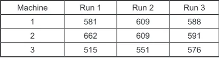
Table 6. Summary of throughput for lathe machines
Machine Run 1 Run 2 Run 3
1 581 609 588
2 662 609 591
throughput of automatic machine 3, it is much desirable to run ANOVA. The result of this sta -tistical step is presented in Table 7. Finally, the statistical summary of the level means of different runs for machine 3 is tabulated in Table 8.
CONCLUSIONS
Productivity model parameters character-istic are based on engineering statcharacter-istical data analyses to establish an appropriate model for
Table 7. Summary of ANOVA for machine 3 throughput
Source DF Adj SS Adj MS F-Value P-Value
Factor 2 36.2 18.11 0.01 0.992
Error 6 13210.7 2201.78 Total 8 13246.9
Table 8. Summary of ANOVA for means of machine 3
Factor N Mean St Dev 95% CI
Run 1 3 586.0 73.6 (519.7, 652.3)
Run 2 3 589.7 33.5 (523.4, 656.0)
Run 3 3 585.00 7.94 (518.71, 651.29)
Fig. 10. Model validation comparison
improving the productivity rate. The process inputs and outputs in the form of factors and re-sponses are branded rendering to variable type that validate the outlay of evidence they cover. It is possible for the process variables to be re-lated with each other deprived of one of them initiating the experimental conduct on the other using the experimental design technique. The current study is based on the relevance of en-gineering statistical approach to analyze three different industrial lathe machines installed in frontier ceramic industry with the intention to replace one of them.
For data value comparison, Minitab 18 was utilized. For sample collection, a suitable time of the day at the start of the morning shift at 9.00 and at the end of the shift at 17.00 was considered to take 10 pieces, two times a day, for three consecutive days from each individual machine while the daily based throughput of all three machines will be exercised accordingly. The relevant machine data have been collected from the maintenance engineering department of the industrial unit. The analysis showed that both machines 1 and 2 have somewhat an equiv -alent inconsistency, but significantly different spreads and locations. Similarly, the throughput for machine 2 was higher with greater variability as compare to machine 1 while machine 3 had encountered significantly more variations with a low rate of throughput. On the other hand, a discussion with concerned machine operator ex-posed that he recognized machine 2 was not set properly. Conversely, he did not need to change machine settings since he knew that a research study was in progress hence was scared he might influence the outcomes by making of adjusting the settings. The operator also pointed out that machine had to be taken down quite a few times for slight maintenance and repairs. On the basis on the basis of the forgoing study analysis fall-outs, the research team has officially suggested to substitute lathe machine 3.
Acknowledgement
This research is fully supported by HEC grant of Research for publishing scientific articles. The author fully acknowledge support from Sarhad university of Science and Information Technol-ogy for the approved fund which makes this im-portant research viable and effective.
REFERENCES
1. Bohannan B.J.M. and R.E. Lenski, The relative im -portance of competition and predation varies with productivity in a model community. The American
Naturalist, 156(4), 2000.
2. Halpern L., M. Koren, and A. Szeidl, Imported in
-puts and productivity. Am. Econ. Rev., 2015. 3. Stock C.A. et al., Reconciling fisheries catch and
ocean productivity. Proc. Natl. Acad. Sci., 2017. 4. Grace J.B. et al., Productivity and plant species
richness. Nature, 2016.
5. Sparke M., B. Mullings, M.W. Wright, K. Derick -son, B.R. Wil-son, and M. Werner, Global Displace-ments: the making of uneven development in the
caribbean. AAG Rev. Books, 5(1), 2017, 74–85.
6. O’Donnell T.J., Productivity and reuse in language. MIT Press, 2015.
7. La Rosa M., W.M.P. Van Der Aalst, M. Dumas, and F.P. Milani, Business process variability modeling. ACM Comput. Surv., 2017.
8. Gröner G., M. Bošković, F.S. Parreiras, and D. Gašević, Modeling and validation of business pro
-cess families. Inf. Syst., 2013.
9. Moses et al., Revisiting a model of ontogenetic growth: estimating model parameters from theory
and data. The American Naturalist, 171(5), 2008. 10. Acernese F. et al., Advanced Virgo: A second-gen
-eration interferometric gravitational wave detector,
Class. Quantum Gravity, 32(2), 2015, p. 024001. .
11. Rozlin N., N. Masdek, A.A. Rozali, M.C. Murad,
and Z. Salleh, Effect of Protein Concentration on Corrosion of Ti-6Al-4V and 316L SS Alloys. ISIJ Int., 58(8), 2018, 1519–1523.
12. Minne E. and J.C. Crittenden, Impact of mainte -nance on life cycle impact and cost assessment for
residential flooring options. Int. J. Life Cycle As
-sess., vol. 20, no. 1, pp. 36–45, Jan. 2015.
13. Beall G. , M. Gallagher, K. House, … S. I.-U. P. A. 12, and U. 2011, “Method and binder for porous
articles”, Google Patents.
14. Sanchez E., F. Gines, J.V Agramunt, and M. Mon
-zo, Clay quality control in tile body production. qualicer.org, pp. 97–112.
15. Gong Y.Z. and H. Liao, Analysis and Research of
Rogowski Coil Current Sensing Technology.Appl.
Mech. Mater., 2014.
16. Hilfiker J.N., J. Sun, and N. Hong, Data analysis. in Springer Series in Optical Sciences, 2018.
17. Srivastava P. and N. Hopwood, A Practical
Itera-tive Framework for QualitaItera-tive Data Analysis.Int. J. Qual. Methods, 2017.
18. Fereday J. and E. Muir-Cochrane, demonstrating
inductive and deductive coding and theme
devel-opment. Int. J. Qual. Methods, 2017.
19. Bumblauskas D., H. Nold, P. Bumblauskas, and A. Igou, Big data analytics: transforming data to
ac-tion. Bus. Process Manag. J., 2017.
20. Kumar R. and R. Kumar, Chapter 10. Data analysis
and interpretation. Nursing Research & Statistics,
2016.
21. Lenting K., R. Verhaak, M. ter Laan, P. Wesseling, and W. Leenders, Glioma: experimental models and reality. Acta Neuropathologica, 2017.
22. Lassmann H. and M. Bradl, Multiple sclerosis:
experimental models and reality. Acta
Neuropatho-logica, 2017.
23. Dunn B., Materials and processes for spacecraft
and high reliability applications, vol. 8, 2016. 24. Urbinati A., D. Chiaroni, and V. Chiesa, Towards a
new taxonomy of circular economy business
mod-els. J. Clean. Prod., 2017.
25. Yang M., P. Smart, M. Kumar, M. Jolly, and S. Evans, Product-service systems business models
for circular supply chains. Prod. Plan. Control,
2018.
26. Zhou L., J. Li, F. Li, Q. Meng, J. Li, and X. Xu, En
-ergy consumption model and en-ergy efficiency of
machine tools: A comprehensive literature review.
Journal of Cleaner Production, 2016.
27. Smalheiser N.R., ANOVA, in Data Literacy, 2017. 28. Randhawa J.S. and I. S. Ahuja, Empirical investi -gation of contributions of 5S practice for realizing improved competitive dimensions, Int. J. Qual.
Re-liab. Manag., 35(3), 2018, 779–810.
29. Chung M.K. Statistical and Computational Meth
-ods in Brain Image Analysis. CRC Press, 2013. 30. Laerd Statistics, One-way ANOVA in SPSS Statis
-tics. Laerd Statistics, 2017.