Implementation and Performance Comparison of Wavelet-Based Filters with the Frequency Domain and Spatial Domain Filters in Destriping of Satellite Images  

Copyright © 2015 CTTS.IN, All right reserved

Implementation and Performance Comparison of

Wavelet-Based Filters with the Frequency Domain and Spatial Domain

Filters in Destriping of Satellite Images

(Case Study: images acquired by the Landsat 4 Multi Spectral

Scanner)

Mohammad Reza Mobasheri

Associate Professor of Remote Sensing Engineering Department, KNToosi University of Technology

Erfan Amraei, Seyyed Amir Zendehbad

MSc Telecommunications Engineering student, Khavaran Institute of Higher Education

Abstract – Nowadays satellite images are widely used to monitor local phenomenon and conduct environmental studies. Unfortunately the existence of some problems in electronic system of the sensors reduces the data quality and appearance of noise in the images. The most common type of noise in these images is the striping noise created as a result of some problems such as the detectors mismatch, improper calibration of the sensor and its fatigue during the lifetime of the satellite. One of the methods to striping noise removal is image filtering. In this paper, we compare the performance of the wavelet based filters, the frequency domain and spatial domain filters in striping noise removal. For this purpose, the images acquired by Landsat 4 Multi Spectral Scanner as well as the simulated images for striping noise are used. Finally, to evaluate the results some statistical parameters such as mean, standard deviation, relative error, RMSE, MSE and PSNR are used that indicate the priority of wavelet-based methods over other methods.

Keyword – Striping Noise, Wavelet Transform, Fourier Transform, Satellite Images, Remote Sensing.

1. I

One of the most important tools used in monitoring environmental phenomena is satellite imaging. Using data collected by satellites it is possible to achieve the up-to-date and reliable date about the environment. Unfortunately in the obtained images by satellite sensors some noise can be seen that origin of them is the sensor’s electronic system. Striping noise is one of the most common noises in these images. Among the factors that cause the striping noise include the improper calibration of the detectors and their mismatch with each other, the failure of detector and worn out sensors [9] [10]. In the sensors that use the wiskbroom imaging technique (such

as MSS1 and MODIS2 sensors striping noise can be seen transversally and alternately [2]. striping noise in images acquired by sensors that use the pushbroom imaging technique (such as the OLI3 and TIRS4 sensors of Landsat 8) are vertical and non-alternately [1]. The existence of striping noise in the images leads to the data destruction and difficulty to extract information from images. Therefore the correction of this type of noise seems necessary. Image de-striping is one of the standard image preprocessing steps that is performed either through sensor calibration and/or image enhancement. In satellite sensors the absolute radiometric calibration is done periodically. sensor detectors frequently deviate from their calibration values, which results in striped images [6]. absolute radiometric calibration provides data that can be used to estimate sensor response, and hence leads to de-striped images. However, cost and logistic issues may reduce the frequency of such calibration. Over the years, many algorithms were developed to de-stripe remote sensing images captured by multiple sensors. Simple Linear Matching (SLM), histogram modification and matching algorithms were one of the earliest methods used for image de-striping [5,8,7]. [3] utilized a moment matching algorithm to de-stripe Landsat satellite imagery. Such algorithms are built on the assumption that each detector views statistically similar. Therefore this method is not applicable in the images that acquired from the scenes with high changes. Additionally, some of the histogram matching algorithms tend to clip the high and low ends of the histograms, which results in a loss of image details. One of the common ways to correct the problems related striping noise is filtering in which the problems of previous methods do not exist in these filters. Filtering methods can be broadly divided into two categories: filtering in

1_{Multi Spectral Scanner}

2

Moderate Resolution Imaging Spectroradiometer

3_{Operational Land Imager} 4

spatial domain, such as convolution filters and, filtering in transformed domain, such as Fourier transform, wavelet decomposition, and Component Analysis [6]. In this study a comparison is made between the performances of the wavelet based, frequency domain and spatial domain filters. For this purpose the images acquired by Landsat 4 MSS sensor are used. To demonstrate the effectiveness of the filters in image de-striping, first the simulated image for striping noise is filtered and the relative error between the original and the filtered image is calculated. Then in the second step the actual images are corrected and some statistical parameters such as mean, standard deviation, MSE1 and PSNR2 are used to assess the results.

2. L

The aim of this study was to design algorithms for image filtering and compare their performance in image de-striping. Wavelet transform as a multi-resolution and scale-space image display is able to separate the directional noise in the wavelet components in a specific direction with different scale levels. However, the Fourier transform only analyzes the image noise within the frequency domain. To analyze the noise in the spatial domain first the image should be analyzed in the frequency domain. Considering that in this study the image is analyzed within these domains, some basic concepts are noted in this section.

2.1. Spatial Domain

In the spatial domain the images are seen as matrix with M × N × T dimensions. In images with gray levels T equals 1. Satellite images are among the images with gray levels. Each element of this matrix is called pixel. Each pixel contains a number that indicates its gray level. The number of gray level depends on the number of bits per pixel. For example for the 8-bit Quants the number of gray levels equal 256. Image filtering in the spatial domain is one method of reducing striping noise in satellite images. Linear filtering of an image is accomplished through an operation called convolution. Convolution is a neighborhood operation in which each output pixel is the weighted sum of neighboring input pixels. The matrix of weights is called the convolution kernel, also known as the filter. The method of applying a convolution kernel to the image is discussed below: A) Rotate the convolution kernel 180 degrees about its center element.

B) The central pixel of convolution kernel is set on the target pixel and the other pixels in the convolution kernel are located on the neighboring pixels of the target pixel. C) Each convolution kernel pixel is multiplied by the corresponding pixel of the image.

D) The final pixel value is equal to the sum of the values obtained in step (c).

1_{Mean Square Error}

2.2. Frequency Domain

Suppose in which x=0, 1, 2, …, M-1 and y= 0, 1, 2, …, N-1 specifies the image. The two-dimensional Fourier transform presented as is obtained from the relation 1 [7]:

= (1)

In fact the Frequency domain is the coordinate system that determined by and the frequency variables u and v. This domain is comparable with the spatial domain (ie the coordinate system defined by the spatial variables x and y). The rectangular M × N area defined by u = 0, 1, 2, ..., M-1 and v = 0, 1, 2, ..., N-1 can be considered as a rectangular frequency. Clearly rectangular frequency has the same size of the input image. Fouriertransformimage is obtainedfrom the following relation[7]:

= (2)

The values in the previous equation are also called the Fourier series coefficients. The value of the Fourier transform in the center of the rectangular frequency ( ) is called dc component of Fourier transform [7]. The general method for visual examination of the Fourier transform is to calculate Fourier spectrum (The value of ) and represent that as an image. If we consider the

and as the real and imaginary parts of transform, Fourier spectrum is defined as the relation 3 [7]:

= (3)

Moreover, the power spectrum is defined as the square of Fourier spectrum. For visual analysis of the Fourier transform there is no difference between Fourier spectrum and power spectrum.

2.3. Wavelet Transform

Wavelet transform represents any arbitrary function as a superposition of wavelets. Unlike Fourier transform, wavelet transform retains both spatial and frequency information. Wavelet transform utilizes narrow groups of wavelets of different shapes that represent local and non-periodic patterns of a signal better than Fourier transform.Unlike the continuous sinusoidal wave function that Fourier uses, a wavelet is a brief oscillation function that is localized in space.Wavelet transform is used in multi-resolution analysis to obtain different approximations of a signal function f(x) at different levels of resolution. For continuous wavelet transform, wavelet coefficient is attained by[6].

u= 0, 1, 2, …, M-1 v= 0, 1, 2, …, N-1

Copyright © 2015 CTTS.IN, All right reserved = (4)

where a and b are scale and translation parameters along x-axis. And function of transform or admissible wavelet is obtained by scaling and translation of a mother wavelet [6]:

= ( ) (5) In discrete signal and according to the dyadic sampling, a and b are considered and k , respectively. Then the wavelet function on an orthonormal basis is defined as [6]:

= (6)

where j and k determine the position and width of wavelet along the x-axis. In multi-resolution analysis, a scaling function is used to create a series of approximations of the function. Wavelet functions are then used to encode the difference in information between approximations. Wavelet function can be expressed as a weighted sum of shifted, double-resolution scaling function [6]:

= (7) where the are called the wavelet function coefficients. The scaling function coefficientcan be related to by the equation = (-1) n . Two-dimensional wavelet transform is a multi-resolution, scale-space representation of 2-D data, such as digital images. It is represented by one scaling function and three directionally sensitive wavelet functions at each scale level [6].

Scalingfunction: =

Wavelet horizontal function: =

Wavelet vertical function: =

Wavelet diagonal function: =

3. M

M

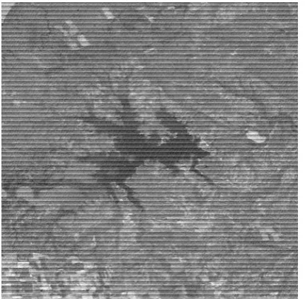
The data used in this study was the level 0 image acquired by Landsat 4 MSS. The image is shown in Figure 1. The striping noise in the images acquired by the MSS sensor occur due to error in the relative gain of the detectors [10]. The difference in relative gain of the detectors causes that the returned values of the individual detectors to be brighter or darker than the return values of the adjacent detectors [10]. It should be noted that the imaging technique in MSS sensor is wiskbroom. Therefore the striping noise in the acquired images by this sensor can be seen in transverse and periodic form.

Fig. 1.Example of striping in Landsat 4 Multispectral Scanner (MSS) Level 0 (L0) data in band 3.

It should be noted that for the calculation and processing MATLAB (MATLAB R2011a) is used.

3.2. Noise Components Detection

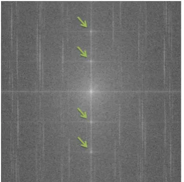
Before designing the filters in spatial and frequency domain the components of the noise must be identified in the frequency domain. To do this we can use the Fourier spectrum or power spectrum. Striping noise leads to the appearance of central narrow bands with high amplitude perpendicular to the stripes in the image Fourier transform and these bands appear as bright spots in Fourier or power spectrum. Therefore, we can amplify the effect of noise to identify its components in the frequency domain. But it should be noted that discrete Fourier transform is calculated only on one periodicity [7]. Calculating two-dimensional discrete Fourier transform creates the points in Figure 2 (a). Shaded areas indicate values that are shown by two-dimensional Fourier transform in equation (1). Like 2 (a), the dotted rectangles shows the reiterative. According to the shaded areas, now includes four back to back quadrant frequencies that meet in the specified point in figure 2(a). By transferring the values in the source to the center of rectangle frequency the visual analysis becomes simple. This can be done by multiplying in . Alternate courses can be arranged like 2 (b). Now the

(a) (b)

Fig. 2. Displaying the Fourier spectrum. a) M × N Fourier spectrum, b) Fourier spectrum transformed into the center of rectangular frequency.

Fig. 3.Fourier spectrum of Figure 1. The bright points in the spectrum indicate the components of the noise.

3.3. Spatial Domain Filter Designing

In this study after the identification of the noise components we used the windowing method in MATLAB for calculating the filter kernel convolution. In this method first the frequency response curve of the ideal filter should be identified. The curve should be the inverse of the noise model in the frequency domain. After determining the ideal filter frequency response curve, the software calculates the convolution kernel in the spatial domain.

As can be seen in Figure 4 (a), the ideal filter frequency response curve is the inverse of the noise model in image Fourier transform. In Figure 4 (b) the actual filter frequency response curve is shown.

(a) (b)

Fig. 4. A) The ideal filter frequency response curve, b) actual filter frequency response curve.

In addition to this filter a Gaussian low pass filter in the spatial domain is used for data filtering.

3.4. Frequency Domain FilterDesigning

Copyright © 2015 CTTS.IN, All right reserved component in order to reduce their amplitude the

Butterworth notch filter in the frequency domain is used. The filter transfer function is presented in equation 8 [7]:

= (8)

In this equation is the notch radius and n is the filter order. and equations are presented in equations 9 and 10 [7]:

= (9)

= (10)

M and N are the image dimensions and , ) are the noise components coordinates. This filter reduces the

noise component amplitude to zero by creating a notch in the noise component coordinate.

3.5. Wavelet-based filter design

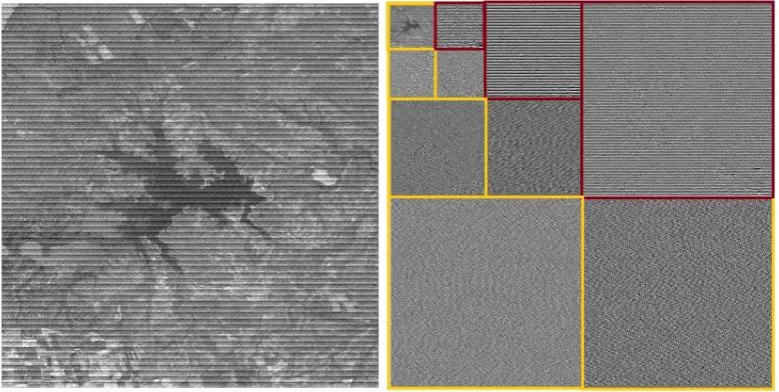
In this method in order to remove striping noise the discrete wavelet transform and adaptive filter in the frequency domain is used. At first, the discrete wavelet is taken from the image and it is decomposed into multi-level frequency scale. In each multi-level in addition to the components of the image approximation, three components of direction (horizontal, vertical and diagonal) are built. This process eliminates the striping in the image (in addition to other image content) from the wavelet components along the striping (for example horizontal striping appear in horizontal minor components). In Figure 5 the wavelet decomposition of 3 levels of Figure 1is shown. Then the directional components of wavelet related to the striping filtered using an adaptive frequency domain filter. The performance of adaptive filter in frequency domain is described below.

Fig. 5. Three-level db4 wavelet decomposition of figure 1

3.5.1. Frequency domain adaptive filter

In this step, the directional wavelet components (vertical or horizontal), corresponding to stripe direction, are transformed to the frequency domain using 1-D Fourier transform. The components are transformed as individual vectors, where each vector contains the digital numbers of a single column or row in the striping direction. For the purpose of this introduction, we will assume that striping occurs in the horizontal direction; hence, we are filtering individual rows in the horizontal component of the image wavelet transform. This process emphasizes the stripes in the frequency domain as variations in the DC (Direct Current or, amplitude value of the zero-frequency) values of the Fourier transform of individual column rows. Generalized frequency filtering can be used at this point to de-stripe the striped directional wavelet components by equalizing the DC value of each

row Fourier transform. One of the approaches that can be used to perform such normalization is to set the DC values to zero (or any constant value). The DC value represents the mean amplitude of the signal row and is proportional to the row mean in the spatial domain. Equalizing the DC values in this sense can introduce artifacts, especially for small images and for images with highly contrasting features. This can lead to errors in the algorithm. To solve this problem an adaptive filter is designed such that during the equalization of DC values in the frequency domain detect the signals without striping noise in the directional wavelet component.

4. R

PSNR, relative error and frequency distribution curves are used. The mathematical relations of each one of these parameters are presented in relations 11-16.

µ = (11)

= (12)

RMSE = (13)

MSE= (14)

PSNR= 10 log[ ] (15)

Relative-Error = (16) In Engineering Science PSNR is a quantity that describes

the ratio between the maximum signal power and destructive noise power. The standard deviation presents the amount of changes or the dispersion from the mean

value. In addition, the mean squared error (MSE) of an estimator measures the mean squared error. The root mean square error (RMSE) indicates the the standard deviation of the difference between the predicted values and the obtained values.

4.2. The evaluation of the results of simulated data correction

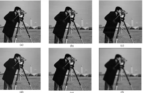
To ensure the effectiveness of the methods presented in this study, the simulated image was filtered. The original and modified images are shown in Figure 6. Table 1 presents the RMSE values and the relative error between the modified images and the image in figure 6 (a).the wavelet based filter is more accurate than other filters. Also the lowest accuracy is related to the low-pass filter. This filter besides noise removal smooth the edges and boundaries that leads to loss of information.

(a) _{(b) (c)}

(d) _(e) (f)

Fig. 6. A) original image, b) simulated image c) corrected image using wavelet-based filter, d) corrected image using order one Butterworth notch filter e) corrected image using spatial domain filter, F) corrected image using Gaussian

low-pass filter with a standard deviation of 2.

Table 1. RMSE and relative error between the corrected images and the image in Figure 6 (a) RMSE Relative error (percent)

Wavelet-based filtering 8.00 6.93

Frequency domain filtering 10:01 8.78

Space domain filtering 11.96 10.99

Low-pass filtering 21:06 18:47

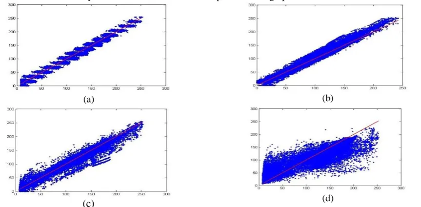
Figure 7 shows the scatter plot between the corrected images and Figure 6 (a). The scatter plot shows the

Copyright © 2015 CTTS.IN, All right reserved images. Ideally, the dispersion is exactly in the first

quarter bisector but in reality these are scattered over a

distance from the first quarter bisector. Distribution of points on the graph confirms the results in Table 1.

(a) (b)

(c) (d)

Figure 7. A) The scatter plot of the pixels of the images in Figure 6 (a) and (c), B) The scatter plot of the pixels of the images in Figure 6 (a) and (d), D) The scatter plot of the pixels of the images in Figure 6 (a) and (e). as presented in this

figure the wavelet-based and frequency domain filters are accurate than the other filters.

4.3. Evaluating the results of the actual image correction

In this part in order to test the methods the image presented in figure 1 is used. The filtering result of this image is presented in figure 8.

(a) _(b)

(c) (d)

Fourier spectrums of the images in figure 8 are presented in Figure 9.

(a) (b)

(c) (d)

Figure 9. A) Fourier spectrum of Figure 8 (a), B) Fourier spectrum of Figure 8 (b), Fourier spectrum of Figure 8 (c), Fourier spectrum of Figure 8 (d).

To measure results the mean parameters and standard deviation were analyzed before and after image

correction. The values obtained for these parameters are shown in Table 2.

Table 2. Mean and SD of the images before and after correction

Mean Standard deviation Figure 1 image (original image) 125.30 31.90

Figure 8 (a) 125.34 21:33

Figure 8 (b) 123.50 21:11

Figure 8 (c) 123.44 20.81

Figure 8 (d) 124.25 16:11

Copyright © 2015 CTTS.IN, All right reserved

(a) (b) (c)

(d) _(e)

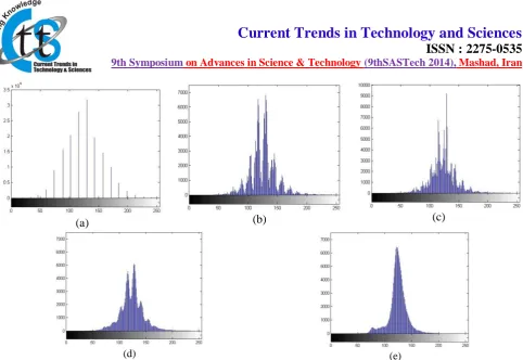
Fig. 10. A) Histogram of Figure 1, B) Histogram of Figure 8 (a), C) Histogram of Figure 8 (b), D) Histogram of Figure 8 (c), E) Histogram of Figure 8 (d).

In the next step the results of figure 1 filtering are compared. To do this, the parameters MSE and PSNR are used. The smaller value obtained for MSE and greater

value obtained for PSNR indicate the higher efficiency of the method. The values obtained for these parameters are shown in Table 3.

Table 3. The values obtained for the MSE and PSNR

MSE PSNR (dB)

Wavelet-based filter 516.01 21.00

Butterworth notch filter 551.39 20.71

Spatial domain filter 586.23 20.45

Gaussian low-pass filter 682.04 19.79

It should be noted that it is possible to change the performance of wavelet and frequency domain filter by changing the decomposition levels, Adaptivefilterthreshold(k) and the filter order. In Figure 11 (a) the diagram of the PSNR changes for different levels of wavelet decomposition is shown based on constant k values. As seen in this figure, the accuracy of

the method is reduced by increased wavelet decomposition levels and adaptive threshold filter. Also in Figure 11 (b) PSNR variation diagram for Butterworth notch filter order is plotted. As seen in this figure, the accuracy of the method is reduced by increasing the filter order.

(a) (b)

5. C

Image filtering is one of the most widely used methods in digital image processing in order to correct the noise. In this study the performance of the wavelet based filter, frequency domain filter and space domain filters were compared in correcting the striping noise in satellite images. For this purpose, the simulated data for the striping noise and the images obtained by the MSS sensor of Landsat4 were used. In order to compare the results of correcting the simulated image the relative error between the primary image and the corrected images were calculated and the lowest error was related to the wavelet based filter and frequency domain filter. In the next step the actual images were corrected. The visual analysis of the corrected images and reduced standard deviation in the corrected images presented the reduced noises compared to the initial image. In the filtered image by low-pass filter besides the noise the main content of image is affected as well. In order to compare the filters the MSE and PSNR parameters were used. The smaller MSE obtained values and greater value obtained for PSNR indicate the higher efficiency of the method. As seen in Table 3, the wavelet based filter and the frequency domain filter are more accurate than the space domain filter.

R

[1] Anger, C., Achal, S., Ivanco, T., Mah, S., Price, R., Busler, J., 1996. Extended operational capabilities of casi. In: Proceedings of the Second International Airborne Remote Sensing Conference, San Francisco, California, 24-27 June, pp. 124-133.

[2] Chander, G., Helder, DL, Boncyk, WC, 2002. Landsat-4/5 BAND 6 relativeradiometry. IEEE Transactions on Geosciences and Remote Sensing 40 (1), 206-210.

[3] Gadallah, FL, Csillag, F., Smith, EJM, 2000. Destriping multisensor imagery with moment matching. International Journal of Remote Sensing 21 (12), 2505-2511.

[4] Gonzalez. R. C, Woods. R. E, Eddins. S. L, "Digital Image Processing Using MATLAB". Beijing: Publishing House of Electronics Industry, 2009.

[5] Horn, BKP, Woodham, RJ, 1979. Destriping LANDSAT MSS images by histogram modification. Computer Graphics and Image Processing 10 (1), 69-83.

[6] Pande-Chhetri. R, Abd-Elrahman.A, De-striping hyperspectral imagery using wavelet transform and adaptive frequency domain filtering, ISPRS Journal of Photogrammetry and Remote Sensing, 66 (2011) 620-636.

[7] Wegener, M., 1990. Destriping multiple detector imagery by improved histogram matching.

International Journal Remote Sensing 11 (5), 859-875.

[8] Weinreb, MP, Xie, R., Lienesch, JH, Crosby, DS, 1989. Destriping GOES images by matching empirical distribution functions.Remote Sensing of the Environment 29 (2), 185-195.

[9] Zhang. M, Carder. K, Muller-Karger. F. E, Lee. Z, Goldgof. D (1999), Noise Reduction and Atmospheric Correction for Coastal Applications of Landsat Thematic Mapper Imagery, Remote Sensing of Environment. 70: 167-180.

[10] 15. Sep. 2014. [online] available: