Active-set Methods for Submodular Minimization Problems
K. S. Sesh Kumar [email protected]
Imperial College London, Department of Computing 180 Queen’s Gate, London SW7 2AZ
Francis Bach [email protected]
INRIA - Sierra Project-team
D´epartement d’Informatique de l’Ecole Normale Sup´erieure (UMR CNRS/ENS/INRIA) 2, rue Simone Iff
75012 Paris, France
Editor:Sebastian Nowozin
Abstract
We consider the submodular function minimization (SFM) and the quadratic minimization prob-lems regularized by the Lov´asz extension of the submodular function. These optimization probprob-lems are intimately related; for example, min-cut problems and total variation denoising problems, where the cut function is submodular and its Lov´asz extension is given by the associated total variation. When a quadratic loss is regularized by the total variation of a cut function, it thus becomes a total variation denoising problem and we use the same terminology in this paper for “general” sub-modular functions. We propose a new active-set algorithm for total variation denoising with the assumption of an oracle that solves the corresponding SFM problem. This can be seen as local descent algorithm over ordered partitions with explicit convergence guarantees. It is more flexible than the existing algorithms with the ability for warm-restarts using the solution of a closely related problem. Further, we also consider the case when a submodular function can be decomposed into the sum of two submodular functionsF1andF2and assume SFM oracles for these two functions. We propose a new active-set algorithm for total variation denoising (and hence SFM by threshold-ing the solution at zero). This algorithm also performs local descent over ordered partitions and its ability to warm start considerably improves the performance of the algorithm. In the experiments, we compare the performance of the proposed algorithms with state-of-the-art algorithms, showing that it reduces the calls to SFM oracles.
Keywords: discrete optimization, submodular function minimization, convex optimization, cut functions, total variation denoising.
1. Introduction
Submodular optimization problems such as total variation denoising and submodular function min-imization are convex optmin-imization problems which are common in computer vision, signal pro-cessing and machine learning (Bach, 2013), with notable applications to graph cut-based image segmentation (Boykov et al., 2001), sensor placement (Krause and Guestrin, 2011), or document summarization (Lin and Bilmes, 2011).
LetF be a normalized submodular function defined onV ={1, . . . , n}, i.e.,F : 2V →Rsuch thatF(∅) = 0and an n-dimensional real vector u, i.e., u ∈ Rn. In this paper, we consider the
c
submodular function minimization (SFM) problem,
min
A⊂V F(A)−u(A), (1)
where we use the conventionu(A) =u>1Aand1A ∈ {0,1}nis the indicator vector of the setA.
Note that general submodular functions can always be decomposed into a normalized submodular function,F, i.e.,F(∅) = 0and a modular functionu(see Bach, 2013).
Let f be the Lov´asz extension of the submodular function F. Let us consider the following continuous optimization problem
min
w∈[0,1]nf(w)−u
>
w. (2)
As a consequence of submodularity, the discrete and continuous optimization problems in Eq. 1 and Eq. 2 respectively have the same optimal solutions (Lov´asz, 1982). Let us consider another related continuous optimization problem
min
w∈Rn
f(w)−u>w+ 12kwk2
2. (3)
IfF is a cut function in a weighted undirected graph, thenf is its associated total variation, hence the denomination oftotal variation denoising(TV) problem for Eq. 3, which we use in this paper— since it is equivalent to minimizing 12ku−wk2
2+f(w). The unique solution of the total variation
denoising in Eq. 3 can be used to obtain the solution of the SFM problem in Eq. 1 by thresholding at0. Conversely, we may obtain the optimal solution of the total variation denoising in Eq. 3 by solving a series of SFM problems using divide-and-conquer strategy.
Relationship with existing work. Generic algorithms to optimize SFM in Eq. 1 or TV in Eq. 3 problems which only access F through function values, e.g., subgradient descent or min-norm-point algorithm (Fujishige, 1984), are too slow without any assumptions (Bach, 2013), as for signal processing applications, high precision is typically required (and often the exact solution).
For decomposable problems, i.e., whenF =F1+· · ·+Fr, where eachFjis “simple”, some
al-gorithms use more powerful oracles than function evaluations, improving the running times. These powerful oracles include SFM oracles that can solve the SFM problem of simple submodular func-tion,Fj given by
min
A⊂V Fj(A)−uj(A), (4)
whereuj ∈ Rn. The other set of powerful oracles are total variation or TV oracles, that solve TV problems of the form
min
w∈Rnfj(w)−u
>
j w+12kwk22, (5)
whereuj ∈Rn. Note that, in general, the exact total variation oracles are at mostO(n)times more expensive than their respective SFM oracle as they solve all SFM problems
min
A⊂V Fj(A)−uj(A) +λ|A|, (6)
cuts) whose total variation oracles are onlyO(1)times more expensive than the corresponding SFM oracles but are still too expensive in practice.
Stobbe and Krause (2010) used SFM oracles instead of function value oracles but their algorithm remains slow in practice. However, when total variation oracles for eachFj are used, they become
competitive (Komodakis et al., 2011; Kumar et al., 2015; Jegelka et al., 2013). Therefore, our goal is to design fast optimization strategies using only efficient SFM oracles for each functionFj rather
than their expensive TV oracles (Kumar et al., 2015; Jegelka et al., 2013) to solve the SFM and TV denoising problems ofF given by Eq. 1 and Eq. 3 respectively. An algorithm was proposed by Landrieu and Obozinski (2016) to search over partition space for solving Eq. 3 with the unary terms
(−u>w)replaced by a convex differentiable function but it applies only to functionsF, which are cut functions.
In this paper, we exploit the polytope structure of these non-smooth optimization problems with exponentially many constraints, i.e., 2n, where each face of the constraint set is indexed by an
ordered partition of the underlying ground set V = {1, . . . , n}. The main insight of this paper is that given the main polytope associated with a submodular function (namely the base polytope described in Section 2) and an ordered partition, we may uniquely define a tangent cone of the polytope. Further, orthogonal projections onto the tangent cone may be done efficiently by isotonic regressions (Best and Chakravarti, 1990). The time needed is linear in the number of elements of the ordered partition used to define the tangent cone. We need SFM oracles only to check the optimality of the ordered partition. Given the orthogonal projectionsonto the tangent cone, if the minimum ofF(A)−s(A)with respect toA⊆V is positive then it is optimal. If it is not optimal, it gives us the violating constraints in the form of active-sets that enable us to generate a new ordered partition among the exponentially many ordered partitions.
Contributions.We make two main contributions:
− Given a submodular functionFwith an SFM oracle, we propose a new active-set algorithm for total variation denoising in Section 3, which is more efficient and flexible than existing ones. This algorithm may be seen as a local descent algorithm over ordered partitions. It has the additional advantage of allowing warm restarts, which will be beneficial when we have to solve a large number of total variation denoising problems as shown in Section 5.
− Given a decomposition of F = F1 +F2, with available SFM oracles for each Fj, we
pro-pose an active-set algorithm for total variation denoising in Section 4 (and hence for SFM by thresholding the solution at zero). These algorithms optimize over ordered partitions (one per functionFj). Following Jegelka et al. (2013) and Kumar et al. (2015), they are also naturally
parallelizable. Given that only SFM oracles are needed, it is much more flexible than the algo-rithms requiring a TV oracle, and allow more applications as shown in Section 5.
2. Review of Submodular Analysis
A set-functionF : 2V → Ris submodular ifF(A) +F(B) > F(A∪B) +F(A∩B)for any subsetsA, B ofV. Our main motivating examples in this paper are cuts in a weighted undirected graph with weight functiona:V ×V →R+, which can be defined as
F(A) =X
i<j
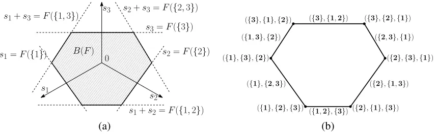
s1+s2=F({1,2})
s1+s3=F({1,3}) s2+s3=F({2,3})
s2=F({2})
s1=F({1})
s3=F({3})
s1
s2
s3
0
B(F)
({3},{1,2})
({2},{1,3}) ({1},{2,3})
({1,3},{2})
({1,2},{3})
({2,3},{1}) ({3},{2},{1}) ({3},{1},{2})
({2},{3},{1})
({2},{1},{3}) ({1},{3},{2})
({1},{2},{3})
(a) (b)
Figure 1: Base polytope forn= 3. (a) definition from its supporting hyperplanes{s(A) =F(A)}. (b) each face (point or segment) ofB(F)is associated with an ordered partition.
wherei, j∈V. Note that there are other submodular functions on which our algorithm works, e.g., concave function on the cardinality set, whichcannotbe represented in the form of Eq. 7 (Ladicky et al., 2010; Kolmogorov, 2012). However, we use cut functions as a running example to better explain our algorithm as they are most widely studied and understood among submodular functions. We now review the relevant concepts from submodular analysis (for more details, see Bach, 2013; Fujishige, 2005).
Lov´asz extension and convexity. The power set 2V is naturally identified with the vertices {0,1}n of the hypercube in n dimensions (going from A ⊆ V to 1
A ∈ {0,1}n). Thus, any
set-function may be seen as a functionf on{0,1}n. It turns out thatf may be extended to the full hypercube[0,1]nby piecewise-linear interpolation, and then to the whole vector spaceRn.
Given a vectorw∈Rn, and given itsuniquelevel-set representation asw=Pmi=1vi1Ai, with
(A1, . . . , Am) a partition ofV andv1 > · · · > vm, f(w) is equal tof(w) = Pmi=1vi
F(Bi)−
F(Bi−1), whereBi = (A1∪ · · · ∪Ai). For cut functions, the Lov´asz extension happens to be
equal to thetotal variation,f(w) =Pi<ja(i, j)|wi−wj|, hence our denomination total variation
denoising for the problem in Eq. 3.
This extension is piecewise linear for any set-functionF. It turns out that it is convex if and only ifF is submodular (Lov´asz, 1982). Any piecewise linear convex function may be represented as the support function of a certain polytopeK, i.e., asf(w) = maxs∈Kw>s(Rockafellar, 1997).
For the Lov´asz extension of a submodular function, there is an explicit description ofK, which we now review.
Base polytope. We define thebase polytopeas
B(F) =s∈Rn, s(V) =F(V), ∀A⊂V, s(A)6F(A) .
Given that it is included in the affine hyperplane{s(V) =F(V)}, it is traditionally represented by the projection on that hyperplane (see Figure 1 (a)). A key result in submodular analysis is that the Lov´asz extension is the support function ofB(F), that is, for anyw∈Rn,
f(w) = sup
s∈B(F)
w>s. (8)
thatwσ(1) ≥ . . . ≥ wσ(n) whereσ represents the order of the elements in V; and (b) computes
sσ(k)=F({σ(1), . . . , σ(k)})−F({σ(1), . . . , σ(k−1)}).
SFM as a convex optimization problem. Another key result of submodular analysis is that mini-mizing a submodular functionF(i.e., minimizing the Lov´asz extensionf on{0,1}n), is equivalent to minimizing the Lov´asz extensionfon the full hypercube[0,1]n(a convex optimization problem). Moreover, with convex duality we have
min
A⊆V F(A)−u(A) = w∈{0,1}min nf(w)−u
>w= min
w∈[0,1]nf(w)−u
>w
= min
w∈[0,1]ns∈B(Fmax)s
>w
−u>w
= max
s∈B(F)w∈[0,1]minns
>
w−u>w= max
s∈B(F) n
X
i=1
min{si−ui,0}.
This dual problem allows to obtain certificates of optimality for the primal-dual pairsw ∈ [0,1]n
ands∈B(F)using the quantity
gap(w, s) :=f(w)−u>w−
n
X
i=1
min{si−ui,0},
which is always non-negative. It is equal to zero only at optimality and the corresponding(w, s)
form an optimal primal-dual pair.
Total variation denoising as projection onto the base polytope.A consequence of the represen-tation off as a support function leads to the following primal/dual pair (Bach, 2013, Sec. 8):
min
w∈Rn
f(w)−u>w+12kwk2
2 = w∈min
Rn
max
s∈B(F)s >w
−u>w+12kwk2
2using Eq. 8,
= max
s∈B(F)w∈minRns
>
w−u>w+12kwk2 2,
= max
s∈B(F)− 1
2ks−uk 2
2, (9)
withw=u−sat optimality. Thus the TV problem is equivalent to the orthogonal projection ofu
ontoB(F).
From TV denoising to SFM. The SFM problem in Eq. 1 and the TV problem in Eq. 3 are tightly connected. Indeed, given the unique solutionwof the TV problem, we obtain a solution of
minA⊆V F(A)−u(A) by thresholdingw at0, i.e., by takingA = {i ∈ V, wi > 0} (Fujishige,
1980).
u
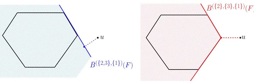
d
B
({2,3},{1})(
F
)
c
B1(F)
u
d
B
({2},{3},{1})(
F
)
Figure 2: Projection algorithm for a single polytope: first projecting on the outer approxima-tion Bb({2,3},{1})(F), with a projected element which is not in B(F) (blue), then on
b
B({2},{3},{1})(F), with a projected element being the projection ofsontoB(F)(red).
3. Ordered Partitions and Isotonic Regression
The main insight of this paper is (a) to consider the detailed face structure of the base polytope
B(F) and (b) to notice that for the outer approximation ofB(F)based on the tangent cone to a certain face, the orthogonal projection problem (which is equivalent to constrained TV denoising) may be solved efficiently using a simple algorithm, originally proposed to solve isotonic regression in linear time. This allows an explicit efficient local search over ordered partitions.
3.1 Outer Approximations ofB(F)
Supporting hyperplanes. The base polytope is defined as the intersection of half-spaces{s(A) 6 F(A)}, for A ⊆ V. Therefore, faces ofB(F) are indexed by subsets of the power set. As a consequence of submodularity (Bach, 2013; Fujishige, 2005), the faces of the base polytopeB(F)
are characterized by “ordered partitions”A= (A1, . . . , Am)withV =A1∪ · · · ∪Am. Then, a face
ofB(F)is such thats(Bi) =F(Bi)for allBi = A1∪ · · · ∪Ai,i= 1, . . . , m. See Figure 1 (b)
for the enumeration of faces forn = 3 based on an enumeration of all ordered partitions. Such ordered partitions are associated to vectorsw=Pmi=1vi1Ai withv1 >· · ·> vmwith all solutions ofmaxs∈B(F)w>sbeing on the corresponding face.
From a face ofB(F)defined by the ordered partitionA, we may define itstangent coneBbA(F)
at this face as the set
b
BA(F) =
n
s∈Rn, s(V) =F(V),∀i∈ {1, . . . , m−1}, s(Bi)6F(Bi)
o
. (10)
Since we have relaxed all the constraints unrelated toA, these are outer approximations ofB(F)as illustrated in Figure 2 for two ordered partitions.
Support function. We may compute the support function ofBbA(F), which is an upper bound onf(w)since this set is an outer approximation ofB(F)as follows:
sup
s∈BbA(F)
w>s = sup
s∈Rn
inf
λ∈Rm−1
+ ×R
w>s−
m
X
i=1
= inf
λ∈Rm−1
+ ×R
sup
s∈Rn
s>w−
m
X
i=1
(λi+· · ·+λm)1Ai
+
m
X
i=1
(λi+· · ·+λm)
F(Bi)−F(Bi−1),
= inf
λ∈Rm−1
+ ×R
m
X
i=1
(λi+· · ·+λm)
F(Bi)−F(Bi−1)
such thatw=
m
X
i=1
(λi+· · ·+λm)1Ai.
Thus, by definingvi = λi +· · ·+λm, which are decreasing, the support function is finite forw
having ordered level sets corresponding to the ordered partitionA(we then say thatwiscompatible
withA). In other words, ifw=Pmi=1vi1Ai, the support functions is equal to the Lov´asz extension
f(w). Otherwise, whenwis not compatible withA, the support function is infinite.
Let us now denote WA as a set of all weight vectorsw that are compatible with the ordered partitionA. This can be defined as
WA=
w∈Rn| ∃v∈Rm, w=
m
X
i=1
vi1Ai, v1 ≥. . .≥vm
.
Therefore,
sup
s∈BbA(F)
w>s=
(
f(w) ifw∈ WA,
∞ otherwise. (11)
3.2 Isotonic Regression for Restricted Problems
Given an ordered partitionA= (A1, . . . , Am)ofV, we consider the original TV problem restricted
towinWA. Since on this constraint setf(w) =Pm i=1vi
F(Bi)−F(Bi−1)is a linear function,
this is equivalent to
min
v∈Rm
m
X
i=1
vi
F(Bi)−F(Bi−1)−u(Ai)
+21Pmi=1|Ai|vi2such thatv1 >· · ·>vm. (12)
This may be done by isotonic regression in complexity O(m) by the weighted pool-adjacent-violator algorithm (Best and Chakravarti, 1990). Typically the solution v will have some values that are equal to each other, which corresponds to merging some setsAi. If these merges are made,
we now obtain a basic ordered partition1 such that our optimalw hasstrictly decreasing values. Because none of the constraints are tight, primal stationarity leads to explicit values ofvgiven by
vi =u(Ai)/|Ai| −(F(Bi)−F(Bi−1))/|Ai|, i.e., givenA, the exact solution of the TV problem
may be obtained in closed form.
Dual interpretation. Eq. 12 is a constrained TV denoising problem that minimizes the cost function in Eq. 3 but with the constraint that weights are compatible with the ordered partitionA,
1. Given a submodular functionFand an ordered partitionA, when the unique solution problem in Eq. 12 is such that
i.e.,minw∈WAf(w)−u>w+1
2kwk 2
2.The dual of the problem can be derived in exactly the same
way as shown in Eq. 9 in the previous section, using the definition of the support function defined by Eq. 11. The corresponding dual is given by maxs∈
b
BA(F)−12ks−uk22,with the relationship w = u−sat optimality. Thus, this corresponds to projectingu onto the outer approximation of the base polytope,BbA(F), which only hasmconstraints instead of the2n−1constraints defining
B(F). See an illustration in Figure 2.
3.3 Checking Optimality of a Basic Ordered Partition
Given a basic ordered partitionA, the associatedw ∈ Rnobtained from Eq. 12 is optimal for the TV problem in Eq. 3 if and only ifs=u−w∈B(F)due to optimality conditions in Eq. 9, which can be checked by minimizing the submodular functionF−s. For a basic partition, a more efficient algorithm is available.
By repeated application of submodularity, we have for all setsC ⊆V, ifCi =C∩Ai:
F(C)−s(C) = F(V ∩C)−
m
X
i=1
s(Ci)(assis a modular function),
= F(Bm∩C)− m
X
i=1
s(Ci) + m−1X
i=1
F(Bi∩C)−F(Bi∩C)(asBm=V),
=
m
X
i=1
F(Bi∩C)−F(Bi−1∩C)−s(Ci)(letB0 =∅and asF(∅) = 0),
=
m
X
i=1
F((Bi−1∪Ai)∩C)−F(Bi−1∩C)−s(Ci)(sinceBi =Bi−1∪Ai),
=
m
X
i=1
F((Bi−1∩C)∪(Ai∩C))−F(Bi−1∩C)−s(Ci),
=
m
X
i=1
F((Bi−1∩C)∪Ci)−F(Bi−1∩C)−s(Ci),
>
m
X
i=1
F(Bi−1∪Ci)−F(Bi−1)−s(Ci)
(as(Bi−1∩C)⊆Bi−1and due to submodularity ofF).
Moreover, we have s(Ai) = F(Bi) −F(Bi−1), which implies s(Bi) = F(Bi) for all i ∈
{1, . . . , m}, and thus all subproblemsminCi⊆AiF(Bi−1∪Ci)−F(Bi−1)−s(Ci)have non-positive values. This implies that we may check optimality by solving thesemsubproblems:sis optimal if and only if all of them have zero values. This leads to smaller subproblems whose overall complex-ity is less than a single SFM oracle call. Moreover, for cut functions, it may be solved by a single oracle call on a graph where some edges have been removed (Tarjan et al., 2006).
Given all sets Ci, we may then define a new ordered partition by splitting allAi for which
F(Bi−1∪Ci)−F(Bi−1)−s(Ci) <0. If no split is possible, the pair(w, s)is optimal for Eq. 3.
in Eq. 12 is strictly lower as shown in Section 3.5 (and leads to another basic ordered partition), which ensures the finite convergence of the algorithm.
3.4 Active-set Algorithm
This leads to the novel active-set algorithm below.
Data: Submodular functionF with SFM oracle,u∈Rn, ordered partitionA Result:primal optimal: w∈Rnand dual optimal:s∈B(F)
1 whileTruedo
2 Solve Eq. 12 using isotonic regression and updateAwith the basic ordered partition ;
3 Check optimality by solvingminCi⊆AiF(Bi−1∪Ci)−F(Bi−1)−s(Ci)for
i∈ {1, . . . , m};
4 ifsis optimalthen
5 break;
6 else
7 fori∈ {1, . . . , m}, split the setAi intoCiandAi\Ciin that order to get an updated
ordered partitionA;
8 end
9 end
Relationship with divide-and-conquer algorithm. When starting from the trivial ordered parti-tionA= (V), then we exactly obtain a parallel version of the divide-and-conquer algorithm (Groen-evelt, 1991), that is, the isotonic regression problem is always solved without using the constraints of monotonicity, i.e., there are no merges, it is not necessary to re-solve the problems where nothing has changed. This shows that the number of iterations is then less thann.
The key added benefits in our formulation is the possibility of warm-starting, which can be very useful for building paths of solutions with different weights on the total variation. This is also useful for decomposable functions where many TV oracles are needed with close-by inputs. See experiments in Section 5.
3.5 Proof of Convergence
In order to prove the convergence of the algorithm in Section 3.4, we only need to show that if the optimality check fails in step (4), then step (7) introduces splits in the partition, which ensures that the isotonic regression in step (2) of the next iteration has a strictly lower value. Let us recall the isotonic regression problem solved in step (2):
min
v∈Rm
m
X
i=1
vi
F(Bi)−F(Bi−1)−u(Ai)
+12|Ai|vi2
(13)
such thatv1 >· · ·>vm. (14)
Steps (2) ensures that the ordered partitionA is a basic ordered partition warranting that the in-equality constraints are strict, i.e., no two partitions have the same valuevi and the values vi for
each element of the partitioni={1, . . . , m}is given through
vi|Ai|=u(Ai)−(F(Bi)−F(Bi−1)), (15)
The optimality check in step (4) decouples into checking the optimality in each subproblem as shown in Section 3.3. If the optimality test fails, then there is a subset of Ci ofAi for some of
elements of the partitionAsuch that
F(Bi−1∪Ci)−F(Bi−1)−s(Ci)<0. (16)
We will show that the splits introduced by step (7) strictly reduces the function value of isotonic regression in Eq. 13, while maintaining the feasibility of the problem. The splits modify the cost function of the isotonic regression as follows, as the objective function in Eq. 13 is equal to
m
X
i=1
vi
F(Bi−1∪Ci)−F(Bi−1)−u(Ci)
+vi
F(Bi)−F(Bi−1∪Ci)−u(Ai\Ci)
+12vi2|Ci|+12v2i|Ai\Ci|
. (17)
Let us assume a positivet ∈ R, which is small enough. The direction that the isotonic regression moves isvi+tfor the partition corresponding toCi andvi−tfor the partition corresponding to
Ai \Ci maintaining the feasibility of the isotonic regression problem, i.e.,v1 > · · · > vi +t >
vi−t>· · ·>vm. The function value is given by
m
X
i=1
(vi+t)
F(Bi−1∪Ci)−F(Bi−1)−u(Ci)
+(vi−t)
F(Bi)−F(Bi−1∪Ci)−u(Ai\Ci)
+12(vi+t)2|Ci|+ 12(vi−t)2|Ai\Ci|
=
m
X
i=1
vi
F(Bi−1∪Ci)−F(Bi−1)−u(Ci)
+vi
F(Bi)−F(Bi−1∪Ci)−u(Ai\Ci)
+12vi2|Ci|+12v2i|Ai\Ci|
+12t2|Ai|
+t 2F(Bi−1∪Ci)−F(Bi−1)−F(Bi)−u(Ci) +u(Ai\Ci) +vi|Ci| −vi|Ai\Ci|
.
From this we can compute the directional derivative of the function att= 0, which is given by
2F(Bi−1∪Ci)−F(Bi−1)−F(Bi)−u(Ci) +u(Ai\Ci) +|Ci|vi− |Ai\Ci|vi
= 2F(Bi−1∪Ci)−F(Bi−1)−F(Bi)−2u(Ci) +u(Ai) + 2|Ci|vi− |Ai|vi
= 2 F(Bi−1∪Ci)−F(Bi−1)−u(Ci) +vi|Ci|
(substituting Eq. 15)
= 2 F(Bi−1∪Ci)−F(Bi−1)−s(Ci)
<0(ass=u−wand Eq. 16).
This shows that the function strictly decreases with the splits introduced in step (7).
3.6 Discussion
Certificates of optimality. The algorithm has dual-infeasible iteratess(they only belong toB(F)
shrinks as we run more iterations of the outer loop. This implies thats∈B(F+ε1Card∈(1,n)), i.e.,
s∈B(Fε)withFε=F+ε1Card∈(1,n). Since by constructionw=u−s, we have:
fε(w)−u>w+12kwk22+ 12ks−uk22 = ε
max
j∈V wj −minj∈V wj
+f(w)−u>w+kwk2
= εmax
j∈V wj −minj∈V wj
+
m
X
i=1
vi
F(Bi)−F(Bi−1)−u(Ai)
+
m
X
i=1
|Ai|v2i
= εmax
j∈V wj −minj∈V wj
( using Eq. 15)
= εrange(w),
where range(w) = maxk∈V wk−mink∈V wk. This means thatw is approximately optimal for
f(w)−u>w+ 12kwk22withcertified gapless thanεrange(w) +εrange(w∗).
Maximal range of an active-set solution. For any ordered partitionA, and the optimal value ofw
(which we know in closed form), we haverange(w)6range(u)+maxi∈V F({i})+F(V\{i})−
F(V) . Indeed, for theupart of the expression, this is because values ofware averages of values ofu; for theF part of the expression, we always have by submodularity:
F(Bi)−F(Bi−1) 6
X
k∈Ai
F({k})and
F(Bi)−F(Bi−1) > −
X
k∈Ai
F(V)−F(V\{k}).
This means that the certificate can be used in practice by replacingrange(w∗)by its upperbound. See experimental evaluation for a 2D total variation denoising in Appendix A.
Exact solution.If the submodular function only takes integer values and we have an approximate solution of the TV problem with gapε6 4n1 , then we have the optimal solution (Chakrabarty et al., 2014).
Relationship with traditional active-set algorithm. Given an ordered partitionA, an active-set method solves the unconstrained optimization problem in Eq. 12 to obtain a value ofv using the primary stationary conditions. The corresponding primal value w = Pmi=1vi1Ai and dual value
s=u−ware optimal, if and only if,
Primal feasibility : w∈ WA, (18)
Dual feasibility : s∈B(F). (19)
If Eq. 18 is not satisfied, a move towards the optimalwis performed to ensure primal feasibility by performing line search, i.e., two consecutive setsAiandAi+1with increasing valuesvi < vi+1
are merged and a potentialw is computed until primal feasibility is met. Then dual feasibility is checked and potential splits are proposed.
4. Decomposable Problems
Many interesting problems in signal processing and computer vision naturally involve submodular functionsF that decompose intoF =F1+· · ·+Fr, withr“simple” submodular functions (Bach,
2013). For example, a cut function in a 2D grid decomposes into a functionF1 composed of cuts
along vertical lines and a function F2 composed of cuts along horizontal lines. For both of these
functions, SFM oracles may be solved inO(n)by message passing. For simplicity, in this paper, we consider the caser = 2functions, but following Komodakis et al. (2011) and Jegelka et al. (2013), our framework easily extends tor >2.
4.1 Reformulation as the Distance Between Two Polytopes
Following Jegelka et al. (2013), we have the primal/dual problems :
min
w∈Rn
f1(w) +f2(w)−u>w+12kwk22 = w∈min
Rn
max
s1∈B(F1), s2∈B(F2)
w>(s1+s2)−u>w+12kwk22
= max
s1∈B(F1), s2∈B(F2)
min
w∈Rn
(s1+s2−u)>w+12kwk22
= max
s1∈B(F1), s2∈B(F2) −1
2ks1+s2−uk 2
2, (20)
withw=u−s1−s2at optimality.
This is the projection ofuon the sum of the base polytopesB(F1) +B(F2) =B(F). Further,
this may be interpreted as finding the distance between two polytopes B(F1)−u/2 and u/2−
B(F2). Note that these two polytopes typically do not intersect (they will if and only ifw = 0
is the optimal solution of the TV problem, which is an uninteresting situation). We now review Alternating projections (AP) (Jegelka et al., 2013), Averaged alternating reflections (AAR) (Jegelka et al., 2013) and Dykstra’s alternating projections (DAP) (Chambolle and Pock, 2015) to show that a large number of total variation denoising problems need to be solved to obtain an optimal solution of Eq. 20. The ability to warm start and solve these total variation denoising using our algorithm in Section 3.4 can greatly improve the performance of each of these algorithms.
Alternating projections (AP).The alternating projection algorithm (Bauschke et al., 1997) was proposed to solve the convex feasibility problem, i.e., to obtain a feasible point in the intersection of two polytopes. It is equivalent to performing block coordinate descent on the dual derived in Eq. 20. Let us denote the projection onto a polytope K asΠK, i.e., ΠK(y) = argmaxx∈K−kx−yk22.
Therefore, alternating projections lead to the following updates for our problem.
zt= Πu/2−B(F2)ΠB(F1)−u/2(zt−1),
wherez0 is an arbitrary starting point. Thus each of these steps require TV oracles for F1 andF2
since projection onto the base polytope is equivalent to performing TV denoising as shown in Eq. 9.
Averaged alternating reflections (AAR).The averaged alternating reflection algorithm (Bauschke et al., 2004), which is also known as Douglas-Rachford splitting can be used to solve convex feasi-bility problems. It is observed to converge quicker than alternating projection (Jegelka et al., 2013; Kumar et al., 2015) in practice. We now introduce a reflection operator for the polytopeKasRK,
given byRK(t) = 2ΠK(t)−t. The updates of each iteration of the averaged alternating reflections,
which starts with an auxiliary sequencez0 initialized to0vector, are given by
zt= 12(I +Ru/2−B(F2)RB(F1)−u/2)(zt−1).
In the feasible case, i.e., intersecting polytopes, the sequenceztweakly converges to a point in the
intersection of the polytopes. However, in our case, we have non intersecting polytopes which leads to a converging sequence ofztwith AP but a diverging sequence ofztwith AAR. However, when
we projectztby using the projection operation,s1,t= ΠB(F1)−u/2(zt);s2,t= Πu/2−B(F2)(s1,t)the sequences s1,t ands2,t converge to the nearest points on the polytopes, B(F1)−u/2andu/2−
B(F2)(Bauschke et al., 2004) respectively.
Dykstra’s alternating projections (DAP).Dykstra’s alternating projection algorithm (Bauschke and Borwein, 1994) retrieves a convex feasible point closest to an arbitrary point, which we assume to be0. It can also be used and has a form of primal descent interpretation, i.e., as coordinate descent for a well-formulated primal problem (Gaffke and Mathar, 1989). Let us denoteιKas the indicator
function of a convex setK. In our case we consider finding the nearest points on the polytopes
B(F1)−u/2andu/2−B(F2)closest to0, which can be formally written as:
min
s∈B(F1)−u2
s∈u
2−B(F2)
1 2ksk
2 2
= min
s∈Rn
1 2ksk
2
2+ιB(F1)−u2(s) +ιu2−B(F2)(s)
= min
s∈Rn
1 2ksk
2
2+ιB(F1)−u2(s) +ιB(F2)−u2(−s)
= min
s∈Rn
1 2ksk
2
2+ max w1∈Rn
w>1s−f1(w1) +
w>1u
2 + maxw2∈Rn−
w2>s−f2(w2) +
w2>u 2
= max
w1∈Rn
w2∈Rn
−f1(w1)−f2(w2) +
(w1+w2)>u
2 + mins∈Rn
1 2ksk
2
2+ (w1−w2)>s
= max
w1∈Rn
w2∈Rn
−f1(w1)−f2(w2) +
(w1+w2)>u
2 −
1
2kw1−w2k
2 2
= min
w1∈Rn
w2∈Rn
f1(w1) +f2(w2)−
(w1+w2)>u
2 +
1
2kw1−w2k
2 2,
wheres=w2−w1at optimality. The block coordinate descent algorithm then gives
w1,t = proxf1−u/2(w2,t−1) = (I−ΠB(F1)−u/2)(w2,t−1),
s1,t = w2,t−1−w1,t,
w2,t = proxf2−u/2(w1,t) = (I −ΠB(F2)−u/2)(w1,t),
s2,t = w1,t−w2,t,
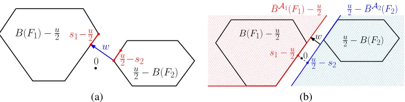
B(F1)−u2
u
2−B(F2)
s1−u2
u
2−s2 0
w
B(F1)−u2 u
2−B(F2)
0
d
BA1(F1)−u
2 u2− d
BA2(F2)
s1−u2 u
2−s2
w
(a) (b)
Figure 3: Closest point between two polytopes. (a) Output of Dykstra’s alternating projection al-gorithm for the TV problem, the pair(s1, s2)may not be unique whilew=s1+s2−u
is. (b) Dykstra’s alternating projection output for outer approximations.
We have implemented it, and it behaves similar to alternating projections, but it still requires TV oracles for projection (see experiments in Section 5). There is however a key difference: while alter-nating projections and alteralter-nating reflections always converge to a pair of closest points, Dykstra’s alternating projection algorithm converges to aspecificpair of points, namely the pair closest to the initialization of the algorithm (Bauschke and Borwein, 1994); see an illustration in Figure 3-(a). This insight will be key in our algorithm to avoid cycling.
Assuming TV oracles are available forF1andF2, Jegelka et al. (2013) and Kumar et al. (2015)
use alternating projection (Bauschke et al., 1997) and alternating reflection (Bauschke et al., 2004) algorithms to solve dual optimization problem in Eq. 20 . Nishihara et al. (2014) gave a extensive theoretical analysis of alternating projection and showed that it converges linearly. However, these algorithms are equivalent to blockdualcoordinate descent and cannot be cast explicitly as descent algorithms for the primal TV problem. On the other hand, Dykstra’s alternating projection is a descent algorithm on the primal, which enables local search over partitions. Complex TV oracles are often implemented by using SFM oracles recursively with the divide-and-conquer strategy on the individual functions. Using our algorithm in Section 3.4, they can be made more efficient using warm-starts (see experiments in Section 5).
4.2 Local Search over Partitions using Active-set Method
Given our algorithm for a single function, it is natural to perform a local search over two partitions A1 and A2, one for each function F1 and F2, and consider in the primal formulation a weight
vector w compatible with both A1 and A2; or, equivalently, in the dual formulation, two outer
approximationsBbA1(F
1) andBbA2(F2). That is, given the ordered partitionsA1 andA2, using a
similar derivation as in Eq. 20, we obtain the primal/dual pairs of optimization problems
max
s1∈BbA1(F1)
s2∈BbA2(F2) −1
2ku−s1−s2k 2
2 = minw∈WA1
w∈WA2
f1(w) +f2(w)−u>w+12kwk22,
withw=u−s1−s2at optimality.
Primal solution by isotonic regression. The primal solutionwis unique by strong convexity. Moreover, it has to be compatible with bothA1 andA2, which is equivalent to being compatible
with thecoalescedordered partitionA= coalesce(A1,A2)defined as the coarsest ordered partition
GivenA, the primal solutionwof the subproblem may be found by isotonic regression like in Section 3.2 in timeO(m)wheremis the number of sets inA. However, finding the optimal dual variabless1 and s2 turns out to be more problematic. We know that s1 +s2 = u−wand that
s1+s2 ∈BbA(F), but the split ofs1+s2into(s1, s2)is unknown.
Obtaining dual solutions. Given ordered partitions A1 and A2, a unique well-defined pair
(s1, s2) could be obtained by using convex feasibility algorithms such as alternating projections
(Bauschke et al., 1997) or alternating reflections (Bauschke et al., 2004). However, the result would depend in non understood ways on the initialization, and we have observed cycling of the active-set algorithm. Using Dykstra’s alternating projection algorithm allows us to converge to a unique well-defined pair(s1, s2)that will lead to a provably non-cycling algorithm.
When running the Dykstra’s alternating projection algorithm starting from 0on the polytopes
b
BA1(F
1)−u/2andu/2−BbA2(F2), ifwis the unique distance vector between the two polytopes,
then the iterates converge to the projection of0onto the convex sets of elements in the two poly-topes that achieve the minimum distance (Bauschke and Borwein, 1994). See Figure 3-(b) for an illustration. This algorithm is however slow to converge when the polytopes do not intersect. Note thatw 6= 0in most of our situations and convergence is hard to monitor because primal iterates of the Dykstra’s alternating projection diverge (Bauschke and Borwein, 1994).
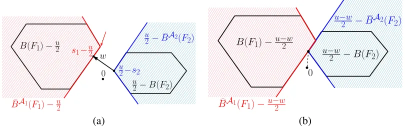
Translated intersecting polytopes. In our situation, we have more to work with than just the ordered partitions: we also know the vector w(as mentioned earlier, it is obtained cheaply from isotonic regression). Indeed, from Lemma 2.2 and Theorem 3.8 from Bauschke and Borwein (1994), given this vectorw, we may translate the two polytopes and now obtain a formulation where the two polytopes do intersect; that is we aim at projecting0on the (non-empty) intersection ofBbA1(F
1)−
u/2 +w/2andu/2−w/2−BbA2(F
2). See Figure 4. We also refer to this as thetranslated Dykstra problem2in the rest of the paper. This is equivalent to solving the following optimization problem
min
s∈BbA1(F1)−u−2w
s∈u−w
2 −BbA2(F2)
1 2ksk
2
2 (21)
= min
s∈Rn
1 2ksk
2
2+ιBbA1(F1)−u−2w(s) +ιu−2w−BbA2(F2)(s),
= min
s∈Rn
1
2ksk22+ιBbA1(F1)−u−2w(s) +ιBbA2(F2)−u−2w(−s),
= min
s∈Rn
1
2ksk22+ maxw1∈WA1 w
>
1 s−f1(w1) +w
>
1(u−w)
2
+ max
w2∈WA2
−w>2s−f2(w2) +
w2>(u−w) 2
,
= max
w1∈WA1
w2∈WA2
−f1(w1)−f2(w2) +
(w1+w2)>(u−w)
2 + mins∈Rn
1 2ksk
2
2+ (w1−w2)>s
,
= max
w1∈WA1
w2∈WA2
−f1(w1)−f2(w2) +
(w1+w2)>(u−w)
2 −
1
2kw1−w2k
2 2
,
B(F1)−u2
u
2−B(F2)
s1−u2
u 2−s2
0
w
d
BA1(F1)−u
2
u 2−
d
BA2(F2)
B(F1)−u−2w
u−w
2 −B(F2) 0
d
BA1(F1)−u−w
2
u−w
2 − d BA2(F2)
(a) (b)
Figure 4: Translated intersecting polytopes. (a) output of our algorithm before translation. (b) Translated formulation.
= min
w1∈WA1
w2∈WA2
f1(w1) +f2(w2)−
(w1+w2)>(u−w)
2 +
1
2kw1−w2k
2 2
, (22)
withs=w2−w1at optimality.
In Section 4.4 we propose algorithms to solve the above optimization problems. Assuming that we are able to solve this step efficiently, we now present our active-set algorithm for decomposable functions below.
4.3 Active-set Algorithm for Decomposable Functions
Data: Submodular functionsF1andF2with SFM oracles,u∈Rn, ordered partitions
A1,A2
Result:primal optimal: w∈Rnand dual optimal:s1∈B(F1), s2 ∈B(F2) 1 whileTruedo
2 A= coalesce(A1,A2);
3 Estimatewby solvingminw∈WAf(w)−u>w+1
2kwk 2
2using isotonic regression ; 4 Projection step:Estimates1∈BbA1(F1)ands2 ∈BbA2(F2)by projecting0onto the
intersection ofBbA1(F
1)−u/2 +w/2andu/2−w/2−BbA2(F2)using any of the
algorithms described in Section 4.4 ;
5 Merge the sets inAjwhich are tight forsj,j∈ {1,2}; 6 Check optimality ofs1ands2as described in Section 3.3; 7 ifs1ands2are optimalthen
8 break;
9 else
10 forj∈ {1,2}andij ∈ {1, . . . , mj}, split the setAj,ij intoCj,ij andAj,ij\Cj,ijin that order to get an updated ordered partitionAj ;
11 end
12 end
Given two ordered partitions A1 and A2, we obtain s1 ∈ BˆA1(F1) and s2 ∈ BˆA2(F2) as
s1 ∈ B(F1) and s2 ∈ B(F2). When checking the optimality described in Section 3.3, we split
the partition. As shown in Appendix C, either (a)kwk2
2 strictly increases at each iteration, or (b)
kwk22remains constant butks1−s2k22strictly increases. This implies that the algorithm is finitely
convergent.
4.4 Optimizing the “Translated Dykstra Problem”
In this section, we describe algorithms for the “projection step” of the active-set algorithm proposed in Section 4.3 that optimizes the translated Dykstra problem in Eq. 22, i.e.,
min
w1∈WA1
w2∈WA2
f1(w1) +f2(w2)−(w1+w2)
>(u−w)
2 +
1
2kw1−w2k2. (23)
The corresponding dual optimization problem is given by
min
s∈BbA1(F1)−u−2w
s∈u−2w−BbA2(F2)
1 2ksk
2
2, (24)
with the optimality conditions=w2−w1. Note that the only link to submodularity is thatf1and
f2are linear functions onWA1 andWA2, respectively. The rest of this section primarily deals with
optimizing a quadratic program and we present two algorithms in Section 4.4.1 and Section 4.4.2.
4.4.1 ACCELERATEDDYKSTRA’SALGORITHM
In this section, we find the projection of the origin onto the intersection of the translated base polytopes obtained by solving the optimization problem in Eq. 22 given by
min
w1∈WA1
w2∈WA2
f1(w1) +f2(w2)−(w1+w2)
>(u−w)
2 +
1
2kw1−w2k 2,
using Dykstra’s alternating projection. It can be solved using the following Dykstra’s iterations:
s1,t = ΠBbA1(F1)(u/2−w/2 +w2,t−1),
w1,t = u/2−w/2 +w2,t−1−s1,t,
s2,t = ΠBbA2(F2)(u/2−w/2 +w1,t),
w2,t = u/2−w/2 +w1,t−s2,t,
with ΠC denoting the orthogonal projection onto the setsC, solved here by isotonic regression.
Note that the value of the auxiliary variable w2 can be warm-started. The algorithm converges
linearly for polyhedral sets (Shusheng, 2000).
In our simulations, we have used the recent accelerated version of Chambolle and Pock (2015), which led to faster convergence. In order to monitor convergence of the algorithm, we compute the value ofku−w−s1,t−s2,tk1, which is equal to zero at convergence. Note that the algorithm is
not finitely convergent and gives onlyapproximatesolutions. Therefore, we introduce the approx-imation parametersε1 andε2 such that s1 lies in the1-neighborhood of the base polytope ofF1,
i.e.,minA⊆V F2(A)−s2(A)≥ −ε2, respectively. See Appendix E for more details on the
approx-imation. The optimization problem can also be decoupled into smaller optimization problems by using the knowledge of the face of the base polytopes on whichs1 ands2 lie. This is still slow to
converge in practice and therefore we present an active-set method in the next section.
4.4.2 PRIMAL ACTIVE-SETMETHOD
In this section, we find the projection of the origin onto the intersection of the translated base polytopes given by Eq. 22 using the standard active-set method (Nocedal and Wright, 2006) by solving a set of linear equations. For this purpose, we derive the equivalent optimization problems using equality constraints.
The ordered partition,Aj is given by(Aj,1, . . . , Aj,mj), wheremjis the number of elements in the ordered partitions. LetBj,ij be defined as(Aj,1∪ · · · ∪Aj,ij). Therefore,
fj(wj) = mj
X
ij=1
vj,ij
Fj(Bj,ij)−Fj(Bj,ij−1)
(25)
wj = mj
X
ij=1
vj,ij1Aj,ij (26)
with the constraints,vj,1 >· · ·>vj,mj. (27)
On substituting Eq. 25, Eq. 26 and Eq. 27 in Eq. 22, we have an equivalent optimization prob-lem:
min
v1,1≥...≥v1,m1
v2,1≥...≥v2,m2
m1
X
i1=1
F1(B1,i1)−F1(B1,i1−1)−
u(A1,i1)−w(A1,i1)
2
v1,i1
+
m2
X
i2=1
F2(B2,i2)−F2(B2,i2−1)−
u(A2,i2)−w(A2,i2)
2
v2,i2
+
m1
X
i1=1
1
2|A1,i1|v
2 1,i1+
m2
X
i2=1
1
2|A2,i2|v
2 2,i2
m1
X
i1=1
m2
X
i2=1
v1,i1v2,i21
>
A1,i11A2,i2.
This can be written as a quadratic program inx =
v1
v2
with inequality constraints in the following form
min
x∈Rm1+m2
D(A1,A2)x<0
1 2x
>Q(
A1,A2)x+c(A1,A2)>x. (28)
Here,D(A1,A2)is a sparse matrix of size(m1+m2−2)×(m1+m2), which is a block diagonal
matrix containing the difference or first order derivative matrices of sizesm1−1×m1 andm2−
1×m2 as the blocks and c(A1,A2) is a linear vector that can be computed using the function
ComputingQ(A1,A2). Let us consider a bipartite graph, G = (A1,A2, E), withm1 +m2
nodes representing the ordered partitions ofA1 andA2 respectively. The weight of the edge
be-tween each element of ordered partitions ofA1, represented byA1,i1 and each element of ordered partitions of A2, represented by A2,i2 is the number of elements of the ground set V that lie in both these partitions and can be written ase(A1,i1, A2,i2) = 1
>
A1,i11A2,i2 for alle∈E. The matrix
Q(A1,A2)represents the Laplacian matrix of the graphG. Figure 5 shows a sample bipartite graph
withm1= 6andm2= 5.
Initializing with primal feasible point. Primal active-set methods start with a primal feasible point and continue to maintain primal feasible iterates. In our case, the starting point may be ob-tained using the weight vectorwthat is estimated using isotonic regression. The vectorwis com-patible both withA1andA2, i.e.,w∈ WA1 andw∈ WA2. Therefore, we may obtain the vectors
v1andv2fromwand initialize the primal feasible starting point usingv1 andv2.
Optimizing the quadratic program in Eq. 28 by using active-set methods is equivalent to finding the face of the constraint set on which the optimal solution lies. For this purpose, we need to be able to solve the quadratic program in Eq. 28 with equality constraints.
Equality constrained QP. Let us now consider the following quadratic program with equality constraints
min
p∈Rm1+m2
D0p=0
1 2p
>
Q(A1,A2)p+ Q(A1,A2)xk+c(A1,A2)
>
p, (29)
whereD0is the subset of the constraints inD(A1,A2), i.e., indices of constraints that are tight and
xk is a primal-feasible point. We refer the indices of the tight constraints as the working setand
represent them by the setW in the algorithm. Therefore, the set of constraints inD0is the restriction of the constraint setD(A1,A2) to the working set constraints denoted byW. The vectorpgives
the direction of strict descent of the cost function in Eq. 28 from feasible point xk (Nocedal and
Wright, 2006).
Without loss of generality, let us assume that the equality constraints are vj,kj = vj,kj+1 for any kj in [0, mj). LetAj0 be the new ordered partition formed by mergingAj,kj and Aj,kj+1 as
vj,kj = vj,kj+1. Similarly, x
0
tcan be computed fromxt by merging the weightsvj,kj andvj,kj+1 into a single weight for the merged element of the ordered partition. Finding the optimal vector
p0 using the quadratic program in Eq. 29 with respect to the ordered partitionA0
j is equivalent to
solving the following unconstrained quadratic problem,
Q(A01,A02, x0t) = min
p0∈
Rm
0
1+m02
1 2p
0>Q(
A01,A02)p0+ Q(A01,A02)x0t+c(A01,A02)
>
p0
, (30)
wherem0jis the number of elements of the ordered partitionA0
j. This can be estimated by solving
a linear system using conjugate gradient descent. The complexity of each iteration of the conjugate gradient is given byO((m01 +m02)k) wherek is the number of non-zero elements in the sparse matrix,Q(A0
1,A02)(Vishnoi, 2013). We can buildpfromp0by repeating the values for the elements
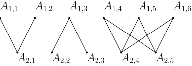
A1;1 A1;2 A1;3 A1;4 A1;5 A1;6
A2;1 A2;2 A2;3 A2;4 A2;5
Figure 5: Bipartite graph to compute Q(A1,A2) with A1 having m1 = 6 components and A2
havingm2 = 5.
Primal active-set algorithm. We now can describe the standard primal active-set method. Data: Laplacian matrix,Q(A1,A2)and vector,c(A1,A2), ordered partitionsA1,A2
Result:x∗∈Rm1+m2
1 Initialize:t= 0;
2 Primal feasiblex0 using the solution of isotonic regressionw; 3 W0with indices of rows ofD(A1,A2)that are equal to 0; 4 whileTruedo
5 Estimate primal: Solve equality constrained QP in Eq. 29 with equality constraints
indexed by working setWtto find optimalp;
6 if p == 0then
7 Estimate dual:λ=D(A1,A2)−> Q(A1,A2)xt+c(A1,A2);
8 if λi ≥0for alli∈Wtthen
9 break;
10 else
11 updatej= argminj∈Wtλj ; 12 updateWt+1=Wt\ {j}; 13 updatext+1 =xt;
14 end
15 else
16 Line search: Find leastβthat retains feasibility ofxt+1 =xt+βpand find the
blocking constraintsBt;
17 Wt+1=Wt∪Bt;
18 end
19 t=t+ 1
20 end
21 returnx∗=xt
We can estimate w1 and w2 fromx∗, which will enable us to estimates feasible in Eq. 24.
Therefore we can estimate the dual variables1∈BA1(F1)ands2 ∈BA2(F2)usings.
4.5 Decoupled Problem
In our context, the quadratic program in Eq. 28 can be decoupled into smaller optimization prob-lems. Let us consider the bipartite graphG= (A1,A2, E)of whichQis the Laplacian matrix. The
Letmbe the total number of connected components inG. These connected components define a partition on the ground setV and a total order on elements of the partition can be obtained using the levels sets ofw. Letkdenote the index of each bipartite subgraph of Grepresented byGk =
(A1,k,A2,k, Ek), wherek= 1,2, . . . , m. LetJkdenote the indices of the nodes ofGkinG.
x∗J
k = argmin
x∈Rm1,k+m2,k
D(A1,A2)kx<0
1 2x
>Q(
A1,A2)JkJkx+c(A1,A2)
>
Jkx, (31)
wheremj,kis size ofAj,k. Therefore,m1,k+m2,kis the total number of nodes in the subgraphGk.
Note that this is exactly equivalent to decomposition of the base polytope ofFj into base polytopes
of submodular functions formed by contractingFj on each individual component representing the
connected componentk. See Appendix D for more details.
5. Experiments
In this section, we show the results of the algorithms proposed on various problems. We first consider the problem of solving total variation denoising for a non decomposable function using active-set methods in Section 5.1, specifically cut functions. Here, our experiments mainly focus on the time comparisons with state-of-art methods and also show an important setting where we show the gain due to the ability to warm-start our algorithm. In Section 5.2, we consider cut functions on a 3D grid decomposed into a function of the 2D grid and a function of chains. We then consider a 2D grid and a concave function on cardinality, which is not a cut function. Our algorithm leads to marginal gains for the usual non decomposable functions. However, in the non decomposable case there are many total variation problems to be solved. The ability to warm-start lends to huge improvements when compared to the usage of standard total variation oracles in this setting.
5.1 Non-decomposable Total Variation Denoising
Our experiments consider images, which are 2-dimensional grids with vertex neighborhood of size 4. The data set comprises of 6 different images of varying sizes. We consider a large im-age of size5616×3744and recursively scale into a smaller image of half the width and half the height maintaining the aspect ratio. Therefore, the size of each image is four times smaller than the size of the previous image. We restrict to anisotropic uniform-weighted total variation to compare with Chambolle and Darbon (2009) but our algorithms work as well with weighted total varia-tion, which is standard in computer vision, and on any graph with SFM oracles. Therefore, the unweighted total variation is
f(w) = λ X
i∼j
|wi − wj|,
whereλis a regularizing constant for solving the total variation problem in Eq. 3.
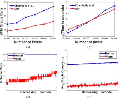
Number of Pixels
2e+04 8e+04 3e+05 1e+06 5e+06 2e+07
SFM Oracle Calls
10 15 20 25 30 35
Chambolle et al. Our
Number of pixels
2e+04 8e+04 3e+05 1e+06 5e+06 2e+07
log(Time in seconds) -4
-2 0 2 4 6 8
Chambolle et al. Our
(a) (b)
Decreasing lambda
# Oracle Calls
2 4 6 8 10 12 14
Normal Warm
Decreasing lambda
Avg Oracle Complexity
0 0.2 0.4 0.6 0.8 1 1.2
Normal Warm
(c) (d)
each call is higher for the our method when compared to Chambolle and Darbon (2009). Figure 6(b) shows the time required for each of the methods to solve the TV problem to convergence. We have an optimized code and only use the oracle as plugin which takes about 80-85 percent of the running time. This is primarily the reason our approach takes more time than (Chambolle and Darbon, 2009) despite having fewer oracle calls for small images.
Figure 6(c) also shows the ability to warm start by using the output of a related problem, i.e., when computing the solution for several values ofλ(which is typical in practice). In this case, we use optimal ordered partitions of the problem with largerλto warm start the problem with smallerλ. It can be observed that warm start of the algorithm requires lesser number of oracle calls to converge than using the initialization with trivial ordered partition. Warm start also largely helps in reducing the burden on the SFM oracle. With warm starts the number of ordered partitions does not change much over iterations. Hence, it suffices to query only ordered partitions that have changed. To analyze this we defineoracle complexityas the fraction of pixels in the elements of the partitions that need to be queried. Oracle complexity is averaged over iterations to understand the average burden on the oracle per iteration. With warm starts this reduces drastically, which can be observed in Figure 6(d).
5.2 Decomposable Total Variation Denoising and SFM
Cut functions. In the decomposable case, we consider the SFM and TV problems on a cut function defined on a 3D-grid. The 3D-grid consists of lines parallel lines in each dimension as shown in Figure 7. It can be decomposed into two functionsF1 andF2, whereF1 is composed on parallel
2D-grids and F2 is composed of parallel chains. From Figure 7, the functionF1 represents all
the solid edges(red and blue) whereas the functionF2 represents the dashed edges(magenta). For
brevity, we refer to each 2D-grid of the functionF1 as aframe. The SFM oracle for the function
F1 is the maxflow-mincut (Boykov and Kolmogorov, 2004) algorithm, which may run in parallel
for all frames. Similarly the SFM oracle for the function F2 is the message passing algorithm,
which may run in parallel for all chains. The corresponding TV oracles, i.e.,projection algorithm
for F1 andF2 may be solved using the algorithm described in Section 3.4 due to availability of
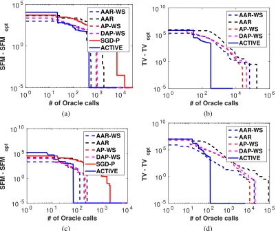
the respective SFM oracles. We consider averaged alternating reflection (AAR) (Bauschke et al., 2004) by solving each projection without warm-start and counting the total number of SFM oracle calls of F1 to solve the SFM and TV on the 3D-grid as our baseline. (SGD-P) denotes the dual
subgradient based method (Komodakis et al., 2011) modified with Polyak’s rule (Poljak, 1987) to solve SFM on the 3D-grid. We show the performance of alternating projection (AP-WS), averaged alternating reflection (AAR-WS) (Bauschke et al., 2004) and Dykstra’s alternating projection (DAP-WS) (Bauschke and Borwein, 1994) using warm start of each projection with the ordered partitions. WS denotes warm start variant of each of the algorithm. The performance of the active-set algorithm proposed in Section 4.3 with inner loop solved using the primal active-set method proposed in Section 4.4.2 is represented by (ACTIVE).
In our experiments, we consider the 3D volumetric data set of the Stanford bunny (max) of size
102×100×79. The functionF1represents102frames whileF2represents the7900chains. The
dimension of each frame inF1is100×79, while the length of each chain inF2is102. Figure 8 (a)
(a) (b) (c)
Figure 7: (a) Cut functionF defined on a 3D-grid may be decomposed into: (b)F1represented by
solid edges (red and blue) and (c)F2 represented by dashed lines (magenta)
# of Oracle calls
100 101 102 103 104
SFM - SFM
opt
10-5 100 105
AAR-WS AAR AP-WS DAP-WS SGD-P ACTIVE
# of Oracle calls
100 102 104 106
TV - TV
opt
10-5 100 105 1010
AAR-WS AAR AP-WS DAP-WS ACTIVE
(a) (b)
# of Oracle calls
100 101 102 103 104
SFM - SFM
opt
10-5 100 105 1010
AAR-WS AAR AP-WS DAP-WS SGD-P ACTIVE
# of Oracle calls
100 101 102 103 104 105
TV - TV
opt
10-5 100 105 1010
AAR-WS AAR AP-WS DAP-WS ACTIVE
(c) (d)
Time comparisons. We also performed time comparisons between the iterative methods and the combinatorial methods on standard data sets. The standard mincut-maxflow (Boykov and Kol-mogorov, 2004) on the 3D volumetric data set of the Standard bunny (max) of size102×100×79
takes0.11seconds while averaged alternating reflections (AAR) without warm start takes0.38 sec-onds. The averaged alternating reflections with warm start (AAR-WS) takes0.21seconds and the active-set method (ACTIVE) takes0.38 seconds. The main bottleneck in the active-set method is the inversion of the Laplacian matrix and it could considerably improve by using methods suggested by Vishnoi (2013). Note that the projection on the base polytopes ofF1andF2can be parallelized
by projecting onto each of the 2D frame ofF1and each line ofF2respectively (Kumar et al., 2015).
The times for (AAR), (AAR-WS) and (ACTIVE) use parallel multi-core architectures3 while the combinatorial algorithm only uses a single core. Note that cut functions on grid structures are only a small subclass of submodular functions with such efficient combinatorial algorithms. In con-trast, our algorithm works on more general class of sum of submodular functions than just with cut functions.
Concave functions on cardinality. In this experiment we consider our SFM problem of sum of a 2D cut on a graph of size5616×3744and a super pixel based concave function on cardinality (Sto-bbe and Krause, 2010; Jegelka et al., 2013). The unary potentials of each pixel is calculated using the Gaussian mixture model of the color features. The edge weighta(i, j) = exp(−kyi −yjk2),
whereyidenotes the RGB values of the pixeli. In order to evaluate the concave function, regions
Rj are extracted via superpixels and, for eachRj, defining the functionF2(S) = |S||Rj\S|. We
use 200 and 500 regions. Figure 8 (c) and (d) shows that (AP-WS), (AAR-WS), (DAP-WS) and (ACTIVE) algorithms converge for solving TV quickly by using only SFM oracles and relatively less number of oracle calls. Note that we count 2D SFM oracle calls.
6. Conclusion
In this paper, we present an efficient active-set algorithm for optimizing quadratic losses regularized by Lov´asz extension of a submodular function using the SFM oracle of the function. We also present an active-set algorithms to minimize sum of “simple” submodular functions using SFM oracles of the individual “simple” functions. We also show that these algorithms are competitive to the existing state-of-art algorithms to minimize submodular functions.
Acknowledgments
We acknowledge support from the European Research Council grant SIERRA (project 239993). K. S. Sesh Kumar also acknowledges the support from the European Research Council grant of Prof. Vladimir Kolmogorov DOiCV(project 616160) at IST Austria. The comments of the reviewers have helped us improve the presentation significantly.
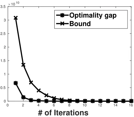
# of Iterations
0 2 4 6 8 10 12 14 16
×1010
0 0.5 1 1.5 2 2.5 3 3.5
Optimality gap Bound
Figure 9: Certified gap vs. bound for TV denoising on a 2D image using the algorithm in Sec-tion 3.4.
Appendix A. Certificates of Optimality
We consider a total variation denoising problem on an 2D image of dimensions384×288using the algorithm proposed in Section 3.4 for non-decomposable functions, where we assume a 2D SFM oracle. Here, we plot the optimality gap given by(f(w)−u>w+12kwk22)−(f(w∗)−u>w∗+
1 2kw
∗k2
2)and the bound,εrange(w)+εrange(w∗), proposed in Section 3.6. Here,wis the solution
at the end of each iteration of the algorithm andw∗is the optimal solution.
Appendix B. Algorithms for Coalescing Partitions
The basic interpretation in coalescing two ordered partitions is as follows. Given an ordered partition A1 andA2 withm1 andm2 elements in the partitions respectively, we define for eachj = 1,2,
∀ij = (1, . . . , mj),Bj,ij = (Aj,1∪. . .∪Aj,ij). The inequalities defining the outer approximation of the base polytopes are given by hyperplanes defined by
∀ij = (1, . . . , mj), sj(Bj,ij)≤Fj(Bj,ij).
The hyperplanes defined by common sets of both these partitions, defines the coalesced ordered partitions. The following algorithm performs coalescing between these partitions.
− Input: Ordered partitionsA1 andA2.
− Initialize:x= 1,y= 1,z= 1andC=∅.
− Algorithm: Iterate untilx=m1andy=m2
1. If|B1,x|>|B2,y|theny:=y+ 1.
3. IfB1,x==B2,ythen
– Az= (B1,x\C),
– C=B1,x, and
– z:=z+ 1.
− Output:m=z, ordered partitionsA= (A1, . . . , Am).
Running time. The algorithm terminates inmin(m1, m2)iterations and the checking condition
for step (3) takesniterations. Therefore, the algorithm overall takes a time ofO(min(m1, m2)n).
Appendix C. Optimality of Algorithm for Decomposable Problems
In step (10) of the algorithms, when we split partitions, the value of the primal/dual pair of opti-mization algorithms
max
s1∈BbA1(F1)
s2∈BbA2(F2) −1
2ku−s1−s2k 2
2 = minw∈WA1
w∈WA2
f1(w) +f2(w)−u>w+12kwk22,
cannot increase. This is because, when splitting, the constraint set for the minimization problem only gets bigger. Since at optimality, we havew=u−s1−s2,kwk2cannot decrease, which shows
the first statement.
Now, ifkwk2remains constant after an iteration, then it has to be the same (and not only have
the same norm), because the optimals1ands2can only move in the direction orthogonal tow.
In step (4) of the algorithm, we project0on the (non-empty) intersection ofBbA1(F
1)−u/2 +
w/2andu/2−w/2−BbA2(F
2). This corresponds to minimizing 12ks1−u/2 +w/2k2such that
s1 ∈ BbA1(F1)ands2 =u−w−s1 ∈ BbA2(F2). This is equivalent to minimizing 81ks1−s2k2.
We have:
max
s1∈BbA1(F1)
s2∈BbA2(F2)
s1+s2=u−w −1
8ks1−s2k
2
2 = min
w1∈WA1
w2∈WA2
max
s1∈Rn
s2∈Rn
s1+s2=u−w
−1
8ks1−s2k
2
2+f1(w1) +f2(w2)
−w1>s1−w>2s2
= min
w1∈WA1
w2∈WA2
max
s2∈Rn
− 1
8ku−w−2s2k
2
2+f1(w1) +f2(w2)
−w1>(u−w−s2)−w>2s2
= min
w1∈WA1
w2∈WA2
max
s2∈Rn
− 18ku−wk22−1 2ks2k
2 2+
1 2s
>
2(u−w)
+f1(w1) +f2(w2)−w1>(u−w−s2)−w2>s2
= min
w1∈WA1
w2∈WA2
−w>1(u−w) +f1(w1) +f2(w2)−
1
8ku−wk
2 2
+ max
s2∈Rn−
1 2ks2k
2
2+s>2 u−w2 +w1−w2
= min
w1∈WA1
w2∈WA2
−w>1(u−w) +f1(w1) +f2(w2)−
1
8ku−wk
−5 −4 −3 −2 −10 0 1 2 3 4 5 2
4 6 8 10 12x 10
4
log(α)
Total inner iterations
−5 −4 −3 −2 −1 0 1 2 3 4 5 120
140 160 180 200
log(α)
# Oracle Calls
50 100 150
0 50 100 150 200 250 300
Outer Iteration
# Inner Iterations
(a) (b) (c)
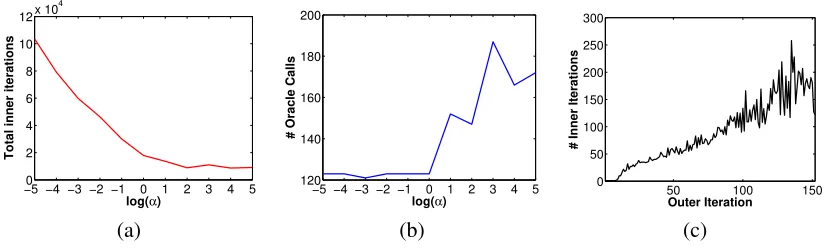
Figure 10: (a) Total number of inner iterations for varyingα. (b) Total number of outer iterations for varyingα. and (c) Number of inner iterations per each outer iteration for theα= 101.
+1 2k
u−w
2 +w1−w2k22
= min
w1∈WA1
w2∈WA2
−w>1(u−w) +f1(w1) +f2(w2) +
1
2kw1−w2k
2 2
+1
2(u−w)
>(w
1−w2)
= min
w1∈WA1
w2∈WA2
f1(w1) +f2(w2)−
1
2(u−w)
>(w
1+w2)
+1
2kw1−w2k
2 2
,
Thuss1 ands2are dual to certain vectorsw1 andw2, which minimize a decoupled formulation in
f1 andf2. To check optimality, like in the single function case, it decouples over the constant sets
ofw1 andw2, which is exactly what step (5) is performing.
If the check is satisfied, it means that w1 and w2 are in fact optimal for the problem above
without the restriction in compatibilities, which implies that they are the Dykstra solutions for the TV problem.
If the check is not satisfied, then the same reasoning as for the one function case, leads directions of descent for the new primal problem above. Hence it decreases; since its value is equal to−18ks1−
s2k22, the value ofks1−s2k22must increase, hence the second statement.
Appendix D. Decoupled Problems.
Given that we deal with polytopes, knowingwimplies that we know the faces on which we have to looked for. It turns outs that for base polytopes, these faces are products of base polytopes for modified functions (a similar fact holds for their outer approximations).
Given the ordered partitionA0defined by the level sets ofw(which have to be finer thanA 1and
A2), we know that we may restrictBbAj(Fj)to elementsssuch thats(B) =F(B)for all sup-level