Convex Analysis for Minimizing and Learning Submodular Set
Functions
Thesis by Peter Stobbe
In Partial Fulfillment of the Requirements for the Degree of
Doctor of Philosophy
California Institute of Technology Pasadena, California
2013
c
2013
Abstract
The connections between convexity and submodularity are explored, for purposes of mini-mizing and learning submodular set functions.
First, we develop a novel method for minimizing a particular class of submodular functions, which can be expressed as a sum of concave functions composed with modular functions. The basic algorithm uses an accelerated first order method applied to a smoothed version of its convex extension. The smoothing algorithm is particularly novel as it allows us to treat general concave potentials without needing to construct a piecewise linear approximation as with graph-based techniques.
Second, we derive the general conditions under which it is possible to find a minimizer of a submodular function via a convex problem. This provides a framework for developing sub-modular minimization algorithms. The framework is then used to develop several algorithms that can be run in a distributed fashion. This is particularly useful for applications where the submodular objective function consists of a sum of many terms, each term dependent on a small part of a large data set.
Contents
List of Figures vii
List of Algorithms viii
1 Introduction 1
1.1 Main Contributions . . . 3
1.2 Outline of Thesis . . . 4
2 Background of Convex Analysis 5 2.1 Basic Concepts. . . 5
2.2 Proximal Operators . . . 8
3 Set Functions and Submodularity 12 3.1 Overview . . . 12
3.2 General Set Functions . . . 12
3.2.1 Set Function Derivatives . . . 14
3.2.2 Monotone and Low Order Functions . . . 16
3.2.3 Fourier Analysis of Set Functions . . . 18
3.2.4 Tensor Product Bases of Set Functions. . . 20
3.3 Properties of Submodular Set Functions . . . 22
3.3.1 Convex Analysis of Submodularity . . . 23
3.3.2 Lovász Extension . . . 27
3.3.3 Examples of Base Polytopes . . . 29
3.4 Submodular Minimization. . . 30
3.4.1 Ellipsoid Method and Polynomial Time Algorithms . . . 31
3.4.3 Special Cases . . . 33
4 Smoothed Gradient Methods for Decomposable Functions 35 4.1 Introduction . . . 35
4.2 Background on Submodular Function Minimization . . . 35
4.3 The Decomposable Submodular Minimization Problem. . . 38
4.4 Classification of Submodular Functions. . . 40
4.4.1 Submodularity of Decomposable Functions. . . 40
4.4.2 Set Cover Functions as Threshold Potentials . . . 41
4.4.3 Reformulation of a Class of Functions . . . 42
4.4.4 Strict Generality of Threshold Potentials . . . 43
4.5 The SLG Algorithm for Threshold Potentials. . . 44
4.5.1 The Smoothed Extension of a Threshold Potential . . . 44
4.5.2 The SLG Algorithm for Minimizing Sums of Threshold Potentials . . . 46
4.5.3 Early Stopping based on Discrete Certificates of Optimality. . . 48
4.6 Extension to General Concave Potentials . . . 50
4.6.1 Formula Derivation . . . 51
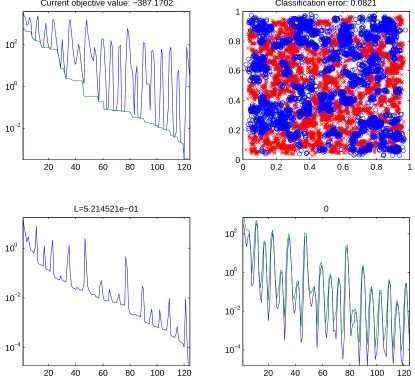
4.7 Experiments . . . 53
4.8 Conclusion . . . 56
5 Distributed Submodular Minimization 57 5.1 Introduction . . . 57
5.2 Submodular Minimization with General Barrier Functions . . . 58
5.3 Consensus Algorithms for Submodular Minimization . . . 63
5.3.1 Notation . . . 63
5.3.2 Outline of Algorithms . . . 64
5.4 Fast Proximal Threshold Potentials . . . 66
5.4.1 General Plane Intersection Projection . . . 66
5.4.2 Box-Plane Projection Algorithms . . . 67
5.5 Experiments . . . 69
6.2 Background. . . 77
6.2.1 The Fourier transform on set functions. . . 77
6.3 Conditions for Recovery . . . 78
6.4 Classes of Set Functions . . . 80
6.4.1 Symmetric functions. . . 81
6.4.2 Low order functions. . . 81
6.4.3 Submodular functions. . . 82
6.5 Reconstruction Algorithms . . . 85
6.5.1 Exploiting structure in the Fourier domain.. . . 86
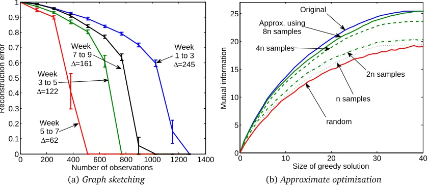
6.6 Applications and Experiments . . . 86
6.6.1 Sketching graph evolution . . . 86
6.6.2 Approximate submodular optimization . . . 88
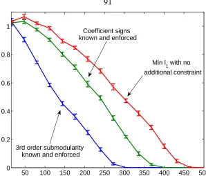
6.6.3 Synthetic Submodular Recovery . . . 89
6.7 Related Work. . . 90
6.8 Conclusion . . . 92
7 Conclusion 94
A Matroid Theory 96
List of Figures
4.1 Example Regions and Comparision of Submodular Minimization Running Times 54
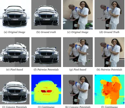
4.2 Segmentation Experimental Results . . . 55
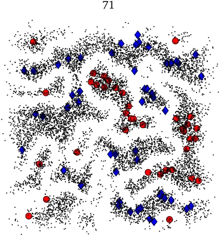
5.1 Synthetic Problem . . . 71
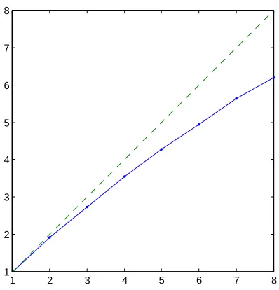
5.2 Parallelization Speedup . . . 72
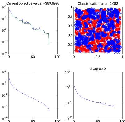
5.3 FISTA convergence . . . 73
5.4 Barzilai–Borwein Convergence . . . 74
6.1 Graph Reconstruction and Approximate Optimization Results . . . 87
List of Algorithms
4.1 SLG: Smoothed Lovász Gradient. . . 48
4.2 Set Generation by Rounding the Continuous Solution . . . 48
4.3 Set Optimality Check. . . 50
4.4 Gradient for General Concave Functions. . . 53
5.1 Projection onto a Box Intersecting a Plane. . . 68
5.2 Piecewise Linear Monotonic Root: Sorted Version . . . 69
Chapter 1
Introduction
There is no doubt that convex optimization has proven to be an invaluable tool throughout all of the applied sciences and engineering. Consider though: the formal definition of convexity is a completely abstract concept, yet somehow has proven to be key in the development of numerical algorithms for countless real-world applications. Given the tremendous track record of such a powerful abstract idea, the mandate of the applied mathematics community must be then to attempt to answer the question: “Can convexity be generalized? Can we discover similar abstract concepts that hold the key for solving new, important problems?” And while one search direction of this quest is to look into the realm of continuous functions for quasiconvex or invex functions as generalizations, the other is to look for discrete analogues of convexity. Indeed, many different such discrete generalizations have been discovered
[Mur03], yet none of them could accurately be described as a perfect mirror image of convexity. But we would claim that there is one such concept from discrete optimization that in recent years has proven to be the most similar to convexity, not only in terms of its salient abstract features, but also its empirical problem solving utility: submodularity.
Submodularity is a property of set functions—meaning functions of some subset of a finite set of objects. It has numerous equivalent definitions, but perhaps the easiest to parse is the following inequality. It says that the change in value of the set function when adding a particular element must be smaller when adding it to a larger1set:
f(A∪ {e})−f(A)≥ f(B∪ {e})−f(B), for all elementseand setsA,Bsuch thate∈/ B⊇A.
mization and minimization with provable guarantees. While both are important, we focus on the latter, as it is in this domain that the connections with convexity are most pronounced. The exact minimum of a submodular function can be found in strongly polynomial time
[IFF01]. This is similar to the fact that convex functions are hard to maximize, but easy to minimize (assuming the convex sets which characterize the problem are not too esoteric). This similarity is is not just a coincidence—the connection between submodularity and convexity goes beyond mere analogy. In fact, submodular functions give rise to a convex interpolant (the Lovász extension) that can be used to minimize the submodular function itself. That is, submodular minimization can be cast as a special type of convex minimization. From a dual perspective, every submodular function corresponds to a convex set, called the base polytope, with a very unique and subtle property. The base polytope is defined by exponentially many inequalities, and yet despite that, one can can find the set of maximizing vertices with respect to any linear function without having to compute any inner products. The resulting exposed face of the base polytope depends only on theorderof the components of the linear function.
Clearly, the connections between submodularity and convexity run deep, and have been known for some time, dating back to at least 1981 with the work of Grötschel, Lovász, and Schrijver[GLS81,Lov83]. Base polytopes (the union of the faces of a polymatroid) were discovered by Edmonds even earlier[Edm70]. Our main goal in this thesis is to explore these connections, but with insight gained from recent advances in convex analysis and sparse reconstruction.
The specific problem that we address, for most of the thesis, is submodular minimization. Despite the known existence of polynomial-time submodular minimization algorithms, the best known exact techniques require a number of function evaluations on the order of n5
and submodular function classes, not unlike the trade-off of generalization in statistics and learning. So in this way, the last major part of the thesis is related to what precedes it. Therein we examine a learning problem, that of set functions. We consider submodular functions in particular as a class of objects to learn, but what sets this work apart from classical research on learning set functions is that we use the tools of convex analysis and sparse recovery.
1.1
Main Contributions
InChapter 4, we develop a novel method for minimizing a particular class of submodular functions, which can be expressed as a sum of concave functions composed with modular functions. The basic algorithm uses an accelerated first order method applied to a smoothed version of the Lovász extension. The smoothing algorithm is particularly novel as it allows us to treat general concave potentials without needing to construct a piecewise linear approxi-mation as with graph-based techniques. This is a fully expanded version of work presented previously[SK10], which did not originally contain the fast method of smoothing.
In Chapter 5, our main technical contribution is elucidating the conditions under which it is possible to find a minimizer of a submodular function via a convex problem. In general one minimizes the Lovász extension together with a separable barrier function, and our Theorem 5.4gives the weakest conditions yet presented in the literature to guarantee that the convex problem gives a minimizer of the submodular problem; we demonstrate why these conditions are necessary, given some mild assumptions. This provides a general framework for developing submodular minimization algorithms. The framework is then used to develop several algorithms that can be run in a distributed fashion. This is particularly useful for applications where the submodular objective function consists of a sum of many terms, each term dependent on a small part of a large data set.
how the assumption of submodularity can be encoded as a constraint of a third order set function and its utility in the reconstruction of a set function.
1.2
Outline of Thesis
• InChapter 2we review some concepts from convex analysis and introduce the notation relevant to convex functions and sets.
• Chapter 3is dedicated to the background material on submodular set functions. Sec-tion 3.2is devoted to the theory of general set functions, whereas inSection 3.3, we review properties of submodular set functions, deriving several of the main relations to convexity. InSection 3.4we discuss submodular minimization.
• InChapter 4we describe our Smoothed Lovász Gradient algorithm for the minimization of decomposable submodular functions. Section 4.4is dedicated to the classification and representation of decomposable functions. This was originally presented in[SK10]. • InChapter 5, we develop consensus algorithms for distributed submodular minimiza-tion. InSection 5.2, we detail the relationship between convex optimization problems and the minimizers of a submodular function.
Chapter 2
Background of Convex Analysis
2.1
Basic Concepts
Throughout this thesis, we will use the convention of convex analysis[Roc70,HUL93,AT03]
that functions are defined everywhere inRn, but functions can equal+∞. When we refer to
the domain of a function, we mean the set of points where it is finite valued:
dom(f):={x∈Rn| f(x)<+∞ }
We define the indicator function of a set to be the function that has that set as its domain, and equals zero there:
δC(x):=
0 x∈C
+∞ x∈/ C
(2.1.1)
This means that there is no loss of generality in treating constrained optimization problems as unconstrained and vice-versa. When we discuss solving minx∈C f(x), whereC is some subset
ofRn, it is equivalent to solving the unconstrained problem minxf(x) +δC(x). (Clearly we
can treat an unconstrained problem as a constrained one with empty constraints.) Convex sets are those which contain every line segment connecting any pair of points in the set. The convex hull of a set is defined as the intersection of all convex sets containing it: convS:=T
C⊆S,
Cconvex
C.
Con-vex functions are not necessarily differentiable, but instead have subgradients. For conCon-vex
f, we define the subdifferential to be the set valued map ∂f :Rn→2Rn which is the set of subgradients: linear functionals which bound the function from below.
∂f(x):={λ∈Rn|f(y)≥ f(x) +〈y−x,λ〉 for all y∈Rn}
Since it is an intersection of half-spaces, the subdifferential is always closed and convex, but it might be empty, even if the function is convex and finite-valued at that point. At any point where a convex function is differentiable, the gradient at that point is the unique subgradient: ∂f(x) ={∇f(x)}. Subdifferentials are linear and positive homogenous, where addition is in
the sense of a Minkowski sum:
∂(f1+αf2) = ∂f1+α ∂f2, α≥0
A key tool in analyzing the dual of a convex program is the convex conjugate, also known as the Legendre-Fenchel transform of a function. It is defined as:
f∗(λ):= sup x∈Rn
〈x,λ〉 −f(x)
This is always convex even if f is not. It is immediate from the definition that:
f(x) +f∗(λ)≥ 〈x,λ〉for allx,λ∈Rn (2.1.2)
Furthermore, note that ifλis a subgradient of f atx, then〈y,λ〉 −f(y)≥ 〈x,λ〉 −f(x)for ally∈Rn. SoEquation 2.1.2holds with equality if and only ifλ∈ ∂f(x).
We denote the set of convex, proper, lower semi-continuous functions as Conv. These functions obey the useful property that they are equal to their biconjugate.
f ∈Conv⇔ f∗∗= f (2.1.3)
So, for f ∈Conv, we can make a stronger statement about whenEquation 2.1.2holds with equality:
One interpretation of Equation 2.1.3is that all f ∈Conv admit the following sort of self-description:
f(x) = sup y,λ
f(y) +〈x−y,λ〉 s.t. λ∈ ∂f(y)
In Section3.3, we show that submodular functions enjoy an analogous property.
The fundamental result for expressing the conjugate of a sum of functions is Fenchel’s theorem.
Theorem 2.1(Fenchel Duality). Suppose the functions fi ∈ConvsatisfyTirelint domfi 6=;.
min x∈Rn
P
i
fi(x) = max
λi∈Rn
−P
i
f∗(λi) s.t. P
i
λi =0
(2.1.4)
Furthermore, the arguments(x∗,λ∗i)are optimal for the above problems if and only if:
λ∗
i ∈ ∂f(x∗), x∗∈ ∂fi∗(λ∗i). (2.1.5)
Relation with Lagrangian Duality. We reformulate as a constrained problem, form the Lagrangian of the constrained problem, and then minimize the Lagrangian to obtain a bound valid for allλi ∈Rn:
min x∈Rn
X
i
fi(x)≥ min
x,xi∈Rn
X
i
fi(xi) +〈x−xi,λi〉=
−P
i fi∗(λi) if
P
iλi =0
−∞ if Piλi 6=0
Note that by assumption, the dual problem is feasible, so the bound involves finite numbers. Likewise, for allx∈Rn, we have:
max P
λi=0
−X
i
f∗(λi)≤ max
λi∈Rn
X
i
〈x,λi〉 −
X
i
f∗(λi) =X
i
fi∗∗(x)
Since fi∗∗ = fi, this means that the theorem gives conditions under which strong duality holds, and a mechanical formula for deriving the dual program.
infimal convolution of functions with the symboland define it by the following formula:
f g(x):= inf
y∈Rn
f(x−y) +g(y)
If f and g satisfy conditions sufficient for Fenchel’s duality theorem to hold, then infimal convolution is essentially the operation which is dual to addition under the Legendre-Fenchel transform: (f g)∗= f∗+g∗ and(f +g)∗=f∗g∗.
2.2
Proximal Operators
A key step in many convex minimization algorithms is solving for the infimal convolution of an objective function with a quadratic function at the current iterate. For any function
f ∈Conv, we define its proximal operator or ‘prox’ as:
proxf(x):=arg min y∈Rn
f(y) +1
2kx−yk
2 (2.2.1)
For a thorough explanation of the proximal operator, see[CP11]. We review a few important ideas and identities.
By strong convexity of the quadratic term, the minimum is a unique point so the prox is well-defined. (In its most general form, one can use any Bregman distance [Brè67]in place of the quadratic, but the present definition is sufficient for our purposes.) The point
p=proxf(x)is uniquely determined by the optimality conditions given by subgradients:
p∈x−∂f(p) (2.2.2)
One way to interpret this equation is that the proximal operator performs an implicit gradient descent step. That is, a basic gradient descent method for convex minimization might use an explicit update rule such as: xk+1=xk−ε∇f(xk), where f is a convex differentiable
From another point of view, the proximal operator is a generalization of projection onto a convex set. When the function f in Equation 2.2.1is the indicator function of a closed convex set (as defined inEquation 2.1.1), then the prox is exactly the projection operator, which we denote with the letterΠ.
ΠC(x):=arg min
y∈C
kx−yk
That is, proxδ
C(x) =ΠC(x).
If we apply Fenchel’s theorem to the proximal problem, we get an important identity relating the prox of a function with the prox of its conjugate. ByEquation 2.1.4, we have for all f ∈Conv:
min y∈Rn
1
2kx−yk
2+f(y) =max
λ∈Rn −1
2kλxk
2− 〈x,λ〉 − f∗(−λ)
Furthermore, byEquation 2.1.5, the optimal arguments satisfyλ∗=y∗−x,y∗∈ ∂f∗(−λ∗),
−λ∗ ∈ ∂f(y∗), so by Equation 2.2.2, we have y∗ = prox
f(x) and −λ∗ = proxf∗(x). We conclude that:
proxf(x) +proxf∗(x) =x (2.2.3) The practical implication of this, from a computational standpoint, is that computing the prox of a function is of the same complexity as computing the prox of its conjugate function.
In particular, consider convex indicator functions and their conjugates, which we denote with the letterσ. These are called the support functions of a set:
σC(x):=sup
λ∈C
〈x,λ〉
We assumeC is a closed convex set, soδ∗∗C =σ∗C =δC. ByEquation 2.2.3, we can compute
the prox forσC by projecting ontoC.
proxσC(x) =x−ΠC(x)
It is clear by definition that support functions are positive homogenous: βσC(x) =σC(βx)
An important special case of a support function is when C is symmetric about the origin and has nonempty interior; if this is true, thenσC is a norm andC is the unit ball of the corresponding dual norm. For example, in the context of sparse approximation, one often minimizes the `1norm to promote sparsity of a vector. The proximal step thus involves subtracting off a projection onto the`∞ ball, which is equivalent to soft thresholding the components of a vector.
Another interesting case is when the support function of a convex set is itself an indicator function of another convex set. It is not hard to see that this is true if and only if the sets are cones. A setKis a cone if it contains all positive multiples of itself:βK⊆Kfor anyβ >0. The corresponding polar coneK◦is defined as the set of the dual vectors which have nonpositive inner product for all points in the cone: K◦:={λ∈Rn| 〈x,λ〉 ≤0 for allx∈K}. If K is
also closed and convex, thenδK ∈Conv, and we haveδ∗K =σK =δK◦. So byEquation 2.2.3, we can rederive a basic result in conic analysis—for any closed convex cone, every point in
Rnis uniquely decomposed as a sum of a point in the cone and a point in the polar cone: x=ΠK(x) +ΠK◦(x).
Prox of a Sum. In general, there is no way to combine and simplify expressions for proximal operators in closed form. However, we can get an implicit characterization of the proximal operator of a sum of functions.
Proposition 2.2. Suppose g is a positive combination of convex functions. Specifically, let
g:=Piωifi wherePiωi=Ω,ωi>0, and fi∈Conv. Thenx=proxg(y)if and only if there are dual vectorsλi such that:
X
i
ωiλi =0 (2.2.4)
x=proxΩf
i(y+λi) for all i (2.2.5)
Proof. To show the forward direction, note that ifx=proxg(y), optimality implies:
0∈x−y+ ∂g(x) = 1
Ω
X
i
ωi x−y+Ω∂fi(x)
By linearity of subgradients, there must existλi satisfyingEquation 2.2.4such that
ByEquation 2.2.2, this is exactly the optimality condition needed to implyx=proxΩf
i(y+λi).
To show the backward direction, note that ifxandλi satisfyEquation 2.2.4and Equa-tion 2.2.5, then
x=arg min z∈Rn
1
2Ωkz−(y+λi)k 2+f
i(z) for all i (2.2.6)
=arg min z∈Rn
X
i
ωi
1
2Ωkz−(y+λi)k 2+f
i(z)
=arg min z∈Rn
1
2kz−yk
2+g(z) =prox
g(y)
Hence,xminimizes each individual term of the sum on the right hand side ofEquation 2.2.6, so thereforexmust minimize the sum of those terms. Within the sum, the dual variablesλi
Chapter 3
Set Functions and Submodularity
3.1
Overview
InSection 3.2, we review some basic concepts from the study of general set functions (not necessarily submodular). We also introduce notation related to set functions that we use throughout the thesis. Insubsection 3.2.1, we define the set function derivative in a way that emphasizes the symmetric shift operator. Insubsection 3.2.2, we define and discuss monotonic functions of general order; this is the natural generalization of submodular to higher order differences. Insubsection 3.2.3, we define the Fourier transform for set functions, a key tool in learning theory of set functions. Insubsection 3.2.4, we define other linear tranforms of variables and show the common connection between them in terms of tensor products.
Finally inSection 3.3, we focus on submodularity in detail. As this material may not be nearly as well-known outside of specialists in combinatorial optimization, we attempt to be more thorough by proving some of the key relationships between submodularity and convexity.
InSection 3.4, we specifically review the problem of submodular minimization, which is the primary subject of theChapter 4andChapter 5. We derive equivalent of a duality gap, and then review some of the existing algorithms.
3.2
General Set Functions
function refers to functions on the cube which take on Boolean values; real-valued functions of Boolean vectors are a generalization called pseudoboolean functions. However, since the power set of a finite set is equivalent to the Boolean cube, in other technical literature the term set function is used. We will use the terminology and notation of sets and set functions, which is more common when the functions are submodular. However, it will be useful to use double brackets[[ ]]to denote the Boolean value of some statement:
[[statement]]:=
1 if the statement is true 0 if the statement is false
Throughout this thesis, we work in some context where there is some finite ground setEof cardinalityn. We letH=R2E be the space of real-valued functions on subsets of E. That is, if f ∈Hthen it is a function f : 2E →R, where 2E is the power set of E. We use the
upper-case letters for subsets ofE, and lowercase letters for elements ofE. Also, we drop brackets for small sets: denoting bor bcrather than{b}or{b,c}when the context is clear. We occasionally use+to mean union, as inA+b+c=A∪ {b} ∪ {c}, but only when the sets are disjoint. When we say that a collection of sets is disjoint, we mean they are pairwise disjoint.
We treat the elements of Eas the indices of vectors inRn. Then for anyA∈2E, we define 1A∈Rnto be the indicator vector of that set.
1A[e]:= [[e∈A]] =
1 ife∈A
0 ife∈E\A
For example, {1e}e∈E is the set of standard unit vectors. Clearly 2E is isomorphic to the
commutative groupZ2nunder the mapping of indicator vectors: 1A+1B≡1A B mod 2. That
is, addition over the group 2Eis the symmetric set difference ( ), defined by:
A B:= (A\B)∪(B\A)
ifA=B. Furthermore, the group of characters ofZn2is used to define the Fourier transform
for set functions, as shown insubsection 3.2.3.
3.2.1 Set Function Derivatives
We now define linear operators on set functions in a way that parallels conventions in, for example, signal processing; this is a slightly different approach than that usually seen in the literature on set functions. We define the (symmetric) shift operatorSB:H→Has the operator which applies a symmetric difference to the argument of a set function:
SBf(A):= f(A B)
If we shift with respect to a singleton we writeSb=S{b}. Clearly these operators are linear and are isomorphic to the group Zn2, meaning that SBSC = SB C. Hence, the operators
commute sinceZn2is commutative. We define the discrete derivative with respect to a single
element as the difference between a shift operator of the element and the identity.
∆b:=Sb−1
Note that the derivative operator has the same function spaceHas its domain and range. A common definition of discrete derivative uses union and intersection rather than symmetric difference, but the advantage of using the symmetric difference is that it is diagonalized by the Fourier transform (i.e., it is a convolution), but the operator defined in terms of unions is not. In any case, the interpretation of the derivative is straightforward; if we evaluate∆bf
on sets that do not contain the element b, we get the change in value of the function due to adding the element:
∆bf(A) = f(A b)− f(A)
So if f is interpreted as a valuation function, then∆bf(A)is the marginal value of itemb
relative to the setA. If we evaluate on a set that already contains b, then the derivative is the change in value from removing the set, which is−1 times the marginal value.
operators with respect to each element in the set:
∆B:=
Y
b∈B
∆b=
Y
b∈B
(Sb−1) (3.2.1)
Because the shift operators commute, this equation does not depend on the ordering of the product, so the above expression for derivative is well-defined. As is the standard convention for empty products, we define∆; to be the identity. It is obvious from our definition that derivatives with respect to disjoint sets combine to form the derivative with respect to their union. That is, assumingB,C disjoint,1we have:
∆B∆C =
Y
b∈B
∆b
Y
c∈C
∆c=
Y
e∈B∪C
∆e=∆B∪C
If we expand out the terms in the product in Equation 3.2.1, we can get an equivalent definition of the derivative as a sum of shift operators:
∆B=
X
C∈2E
[[C⊆B]] (−1)|B|+|C|SC
For example, the derivative with respect to a pair of elements∆bc=∆{b,c} equals:
∆bcf(A) = f(A bc)−f(A b)−f(A c) + f(A)
This also called the second order difference operator. Note that there is also a product rule for discrete derivatives:
Lemma 3.1(Product Rule for Set Function Derivatives).
∆B(f g) =
X
C∈2E
[[C⊆B]] (∆Cf)(SC∆B\Cg) (3.2.2)
Proof. When|B|=1, this is true by the following identity:
∆b(f g) = (Sbf −f)Sbg+f(Sbg−g)
= (∆bf)(Sb∆;g) + (∆;f)(S;∆bg)
1Since(∆
If|B|>1, iterating over all elements b∈Bresults inEquation 3.2.2.
3.2.2 Monotone and Low Order Functions
With our definition of derivative, we can define the cones of orderq monotone functions, which we denoteH+q (resp. H−q). It is the subset of functions with all orderqderivatives nonnegative (resp. nonpositive). With a slight overload of notation, we will use the symbol ±rather than state all equations forH+q andH−q separately.
H±q :={f ∈H| ±∆Bf(A)≥0 for allA,B∈2Ewith A∩B=;,|B|=q}
The first few of these cones have more common names, and simple alternate characterizations: • H±0 nonnegative/nonpositive: ±f(A)≥0
• H±1 nondecreasing/nonincreasing: ±(f(A∪B)−f(A))≥0
• H±2 supermodular/submodular: ±(f(A∪B∪C)−f(A∪B)−f(A∪C) + f(A))≥0
Note that the characterizations we list involve adding and removing entire sets rather than just single elements. This fact generalizes nicely to higher order monotone functions. Informally, the following proposition states that for aqmonotone function, we can replace the singleton sets that occur in the definition of the discrete derivative (Equation 3.2.1) with general disjoint sets, and still get a valid inequality.
Proposition 3.2. The function f is inH±q if and only if for all collections of q+1disjoints sets A,B1, . . .Bq, we have:
±
q
Y
i=1
SB i−1
f(A)≥0 (3.2.3)
Proof. Clearly if C is an arbitrary subset of sizeq, disjoint fromA, we can choose each of the setsBi to be singletons such that C=B1+. . .+Bq, which implies the operator product in Equation 3.2.3is the set derivative with respect toC. Hence f ∈H±q.
B(i)for j=1 . . .|Bi|. Then each term in the product can be expressed as a telescoping sum:
SBi−1=
|Bi| X
j=1
SB(i,j)−SB(i,j−1)= |Bi| X
j=1
SB(i,j−1)∆c(i,j)
By substituting this equivalence into the each term in the the product fromEquation 3.2.3, and then expanding the sum out to|B1|. . .|Bq|terms, we get:
±
q
Y
i=1
SB i−1
f(A) =±
q
Y
i=1
|Bi| X
j=1
SB(i,j−1)∆c(i,j)f(A) = X
j1,...,jq
±SB0(j
1,...jq)∆C0(j1,...jq)f(A), B0(j1, . . .jq):=∪qi=1B(i,ji−1), C0(j1, . . .jq):={c(i,ji)}qi=1.
Note that for each term in the series, the argumentA, shifting setsB0and derivative setsC0
are disjoint. Also each setC0 is of sizeq. Therefore, the expression fromEquation 3.2.3is equivalent to a sum of orderq derivatives. Since f ∈H±q implies that orderq derivatives are uniformly nonnegative (resp. nonpositive), the entire sum is nonnegative.
This result is included in[FH05]but given as a symmetric statement over collections ofk
general sets, not necessarily disjoint. Given general setsC1, . . . ,Cq, this definesq+1 disjoint sets as follows: A=Tqj=1Cj,Bi =Tj6=iCj\Ci. Then by applying the above Proposition to the disjoint sets, we get the result in the form stated in[FH05]:
±(−1)q
f ∩qj=1Cj+ X
J⊆{1,...,q}
J6=;
(−1)|J|f ∪i∈J∩j6=i Cj
≥0.
Products of Monotonic Functions. Due to the product rule ofEquation 3.2.2, we can get simple rules for classifying products of functions if they obey certain patterns of monotonicities. To express the following lemma, we will need variables to be signs: {+,−}. For these purposes they are equivalent to the unit numbers{+1,−1}.
Lemma 3.3. Suppose f,g∈Hare monotonic for every order up to order q:
f ∈Hs0
0 ∩. . .∩H
sq
q, g∈H t0
0 ∩. . .∩H
tq
q .
f g∈Hγq.
Proof. Let B be any set of size q. We use the product rule (Equation 3.2.2) to take the derivative of f gwith respect toB. For simplicity we do not write the argumentA, but assume it is disjoint fromB. Within the resulting sum, we use the factorizationγ=sktq−k:
γ∆B(f g) =
X
C∈2E
[[C⊆B]]γ(∆Cf)(SC∆B\Cg)
=
q
X
k=0
X
C∈2E
[[C ⊆B,|C|=k]] (sk∆Cf)(tq−kSC∆B\Cg)
For|C|=k, we havesk∆Cf ≥0 since f ∈Hsk
0 and tq−kSC∆B\Cg≥0 since f ∈H tq−k
q−k and
|B\C|=q−k. So each term in the sum multiplies to a nonnegative sign. Thusγ∆B(f g)≥0
for arbitraryBof sizeq, so indeed f g∈Hγq.
For example, if f is nonnegative, nondecreasing, submodular (H+0∩H+1 ∩H−2), andg is nonnegative nonincreasing submodular (H+0∩H−1∩H−2), then the product f gis nonnegative submodularH+0 ∩H−2, but neither increasing nor decreasing in general. Another example of Lemma 3.3 is that the cone of nonnegative, nondecreasing, supermodular functions (H+0 ∩H+1∩H+2) is closed under multiplication.
We defineq-th order functions, as functions with all derivatives beyond orderq equal to zero.
Hq:={f ∈H|∆Bf(A) =0 for allA,B∈2Ewith |B|>q}
It is easy to see from the definition that:Hq=H+q+1∩Hq−+1andHq⊂Hq+1. The set of zeroth order functions are constant functions. In the context of set functions, first order functions are known as modular, and admit the description: f(A) =f(;) +Pa∈A(f(a)−f(;)).
3.2.3 Fourier Analysis of Set Functions
In this section, we briefly introduce the Fourier transform for set functions, but it is primarily expanded upon inChapter 6. The characters of the group 2Ecan be written as ψ
B(A):=
normalized inner product with such functions:
b
f(B):= 1 2|E|
X
A∈2E
f(A)ψB(A)
This is an orthogonal transform, so though the inverse formula has a different normalization constant, it is otherwise the same: f(A) =PB∈2E bf(B)ψB(A). One way to interpret the
Fourier coefficient for a set is that it is the average of all the derivatives with respect to that set (modulo a factor of−1 for odd sets).
b
f(B) = (−1) |B|
2|E\B| X
A∈2E
[[A⊆E\B]]∆Bf(A) (3.2.4)
Next, we define convolutions of set functions:
f ∗g(A):= X
B∈2E
f(A B)g(B)
This satisfies the standard properties of a convolution: Commutivityf∗g=g∗f, Associativity, (f ∗g)∗h= f ∗(g∗h), Linearity(αf +βg)∗h=α(f ∗h) +β(g∗h). Also, convolution in the time domain is multiplication in the Fourier Domain, and vice-versa.
Öf ∗g(B) =2nfb(B)bg(B), Óf g(B) = (bf ∗bg)(B).
The advantage of our definition for set function derivatives is that it is just a convolution. That is,∆Cf =f ∗g where g(A) = [[A⊆C]] (−1)|A|+|C|, and 2nbg(B) = [[C⊆B]] (−2)|C|. So a derivative can be treated as a sort of high-pass filter. After taking the derivative with respect to
C, all coefficients which are not subsets ofCare zeroed out: ∆ÕCf(B) = [[C⊆B]](−2)|C|fb(B).
This gives us a formula to express a derivative as a sum of Fourier coefficents:
∆Cf(A) = (−2)|C|
X
B∈2E
[[C⊆B]]bf(B)ψB(A) (3.2.5)
q. That is:
Hq={f ∈H|fb(B) =0 for all|B|>q}
The bestq-th order approximation for a set function in an`2sense is given by setting all higher order Fourier coefficients to zero: g =arg ming0∈H
qkf −g 0k ⇔
b
g(B) = [[|B| ≤q]] bf(B).
This is immediate from the fact that the Fourier transform is an isometry. See[HH92]and
[GMR00]for the formulas of this operation in terms of different function bases.
In elementary signal processing, the domains analyzed are the continuous/discrete circle/line (Zn,[0, 1],Z, orR). Exactly as there, (periodic) shifting, derivatives, and low
pass filtering can all be expressed as convolutions, so unsurprisingly these operations all commute with each other.
3.2.4 Tensor Product Bases of Set Functions
In addition to the standard basis and the Fourier transform, there are several other useful bases for representing set functions. For a thorough discussion, see [GMR00], but let us review two of the more important ones. The feature common to all the bases that we present is that they can be expressed easily through tensor products.
Möbius Transform and Boolean Polynomials. One way to represent set functions is as a multilinear (a.k.a. polynomial) function over the Boolean cubep(x) =p0+p1x[1]+p2x[2]+ . . .p1...nx[1]. . .x[n]. This gives a simple way to interpolate a set function continuously
over the unit cube by letting the variablextake on values[0, 1]n ⊂Rn. In this case, the
interpolation is multilinear by convention since Booleans satisfy x2=x, and so there is no reason to include nonlinear terms such as x[i]2.
To calculate the coeffcient of a polynomial that represents a set function, we evaluate the set function derivative at the empty set. A set function derivative is exactly the stencil of a mixed derivative of anndimensional function; an orderqdiscrete derivative is the forward difference operator tensored in some set ofq dimensions. Since the Boolean polynomial is multilinear, in general, set function derivatives equal the continuous partial derivatives exactly (provided the argument set and derivative set are disjoint). For example: suppose
E={1, 2, 3}, and the set function f is related to the Boolean polynomialpby f(A) =p(1A).
mixed partial derivative of pat the corresponding corner: ∆12f(3) =D12p(13) =p12+p123. The transformation from set function values to polynomial coefficients is sometimes called the Möbius transform. We can express this not only as a set derivative, but also we can useEquation 3.2.5to equate it with a sum of Fourier coefficients.
g(B) =∆Bf(;) = (−2)|B|X
C
[[B⊆C]]fb(C)
f(A) = X
B
[[B⊆A]]g(B)
Disjuction. Functions of the form min(1,|A∩B|)are equivalent to a disjunction (Boolean OR) operation. A sum of such functions is equivalent to a set cover function, as described in subsection 4.4.2. These functions do not quite form a basis ofH, since they all have f(;) =0. But by including a constant offset, we get a basis forH. The corresponding analysis and synthesis formulas are:
h(B) =−∆Bf(E) =−2|B|∆E\Bbf(E) f(A) = f(;) +X
B
min(1,|A∩B|)h(B)
There is an interesting consequence to the formula relating the set cover coefficients to Fourier coefficients. The original function f is set cover representable (meaning it can be expressed as a nonnegative combination of such functions, so thath(B)≥0 for all nonemptyB) if and only if the Fourier coefficients fb(B)for nonempty sets are nonpositive and nondecreasing.
Tensor Product Notation. The above formulas may seem a bit mysterious and hard to check for correctness. However, the calculations are fairly simple if you consider set functions as vectors inR2
n
, since all of the bases we have described can be expressed in terms ofn-fold tensor products of 2×2 matrices. Let us denote(⊗n)for the operation of tensoring a matrix with itselfntimes. Then the main formulas of this section can be written as:
Fourier: fb=
1/2 1/2 1/2 −1/2
⊗n
f, f =
1 1
1 −1
⊗n b f.
Möbius: g=
1 0
−1 1
⊗n
f, f =
1 0 1 1
Disjunction: h=−
0 1
1 −1
⊗n
f, f = f(;) +
1 1 1 1
⊗n
−
1 1 1 0
⊗n h.
Therefore, it is straightforward to derive the basic formulas relating different tensor product bases by simply inverting and/or multiplying 2×2 matrices.
3.3
Properties of Submodular Set Functions
There are many equivalent characterizations of submodularity. As we have already introduced the notion of set derivative, we give a few which are directly related to set derivatives:
1. f(A+b+c)−f(A+b)−f(A+c) +f(A)≤0, for allb,c∈E, A⊆E−b−c. 2. f(A∪B∪C)−f(A∪B)−f(A∪C) + f(A)≤0, for allA,B,C disjoint. 3. f(A∩B) +f(A∪B)≤f(A) +f(B)for allA,B∈2E.
4. f(A+c)−f(A)≥ f(B+c)− f(B)for all c∈E, A⊆B⊆E−c. There are n
2
2n−2different inequalities to check in item 1. This is the minimum number of inequalities needed to check submodularity in general. That is, no subset of these inequalities implies any other subset of them. Theorem3.2gives the characterizations of items 2. The interpretation of item 4 is that first order differences are decreasing functions. It is an easy consequence of item 3. To test submodularity, it is generally easiest to use item 1. Besides the fact that it has fewer inequalities to check, each inequality involves the change in value when adding only 2 elements to a set.
These properties seem fairly similar in that they involve inequalities of the set derivatives. However, there are several other characterizations, some of which appear to have nothing to do with second order differences being negative. For example, a set function f is submodular if and only if for all c ∈ Rn it holds thatA,B ∈ Qc ⇒A∩B, A∪B ∈ Qc, where Qc :=
arg minAf(A) +〈1A,c〉. In words, this means that the collection of minimizers of f plus any
modular function is a lattice. See[Fuj05]for a proof. Another example of a rather striking necessary and sufficient condition for submodularity is given in Proposition3.4.
constraint can be done to within a constant factor of the optimum. That is, if one wishes to find a maximal set of sizek, then a simple greedy algorithm2will give a set of cardinalityk
with function value no less than 1−1/eof the maximal set of cardinalityk[NWF78]. This useful property of approximate maximization is is a major driving force behind the interest in submodular functions, as it has many practical applications and useful generalizations. However, aside from our experiments showcased inFigure 6.1, we otherwise focus on the problem of submodular minimization.
3.3.1 Convex Analysis of Submodularity
We give an overview of how convex analysis can be used to analyze submodular functions. While this presentation is original, the material is standard[Sch03,Fuj05,Bac11].
We start by defining some important polyhedra used in the analysis of submodular functions. We can define the subdifferential of a set function in a form analogous to continous functions, except modular set functions play the role of linear functionals. Any vectorλ∈Rn
defines a modular function on E, which we can denote in different ways, depending on what is convenient for the context:
2E3A7→λ(A):=〈1A,λ〉=
X
a∈A
λ[a]
Then the subdifferential of a set function at a set is defined as a modular function which lower bounds the change in value of the function relative to that set. That is,λis subgradient for f at the setA, if for all setsBthe difference f(B)− f(A)is bounded below by difference λ(B)−λ(A).
∂f(A):={λ∈Rn|f(B)≥ f(A) +〈1B−1A,λ〉for allB∈2E}
We also refer to this as the discrete subdifferential. Unlike a continuous subdifferential, which may be empty if a function is nonconvex, the discrete subdifferential is always nonempty. In fact, the subdifferential for the setAis unbounded along every ray in the direction1A−1E\A.
This is true foranyset function. This is because ∂f(A)is a polyhedron defined by the normal directions1B−1A where B ∈2E\ {A}, and for any such direction〈1B−1A,1A−1E\A〉 =
−|A B| < 0. So moving far enough in the direction 1A−1E\A will always result in a
subgradient. Precisely, for anyλ∈Rn, we have:
λ+t(1A−1E\A)∈ ∂f(A) ⇔ t≥max B∈2E
B6=A
f(A)−f(B) +λ(B)−λ(A)
|A B|
In what follows, we will assume that the set function f is ‘normalized’, it has f(;) = 0, possibly by subtracting an offset. The submodular polyhedronPf and base polytope Bf are thus defined by:
Pf :={λ∈Rn| 〈1A,λ〉 ≤ f(A)for allA∈2E} (3.3.1)
Bf :={λ∈Rn| 〈1,λ〉= f(E), and〈1A,λ〉 ≤ f(A)for allA∈2E} (3.3.2)
It is easy to see that thatPf = ∂f(;). Furthermore,
Pf ∩∂f(A) =Pf ∩ {λ∈Rn|λ(A) = f(A)}
In particular,Bf = ∂f(;)∩∂f(E). Note that all vectors in the setBf must satisfyλ[a]≤ f(a)
and〈1,λ〉= f(E), and thusλ[b]≥ f(E)−Pa∈E−bf(a). So the set Bf is bounded and we
are justified in referring to it as a polytope. The elements of the base polytope are called the bases of the function. Note when f is the rank function of a matroid (cf. Appendix A), each extreme point of the base polytope corresponds to the indicator vector of a base (a.k.a. basis) for the matroid.
The base polytope essentially contains all the subgradients needed to fully characterize a submodular function. While it is defined by exponentially many constraints, there is a simple formula to optimize a linear function over it if we have oracle access to the function, if and only if the function is submodular. The key insight due to Edmonds[Edm70]is that solving maxλ∈B
f〈x,λ〉depends only on the ordering of the components ofx.
its polar cone.
Kπ:={x∈Rn|x[π1]≥x[π2]. . .≥x[πn]} (3.3.3)
Kπ◦:={λ∈Rn| 〈1,λ〉=0, and Pki=1λ[πi]≤0 fork=1 . . .n} (3.3.4)
Note that these cones are proper with respect to the subspace of vectors orthogonal to1. Given a permutationπ, consider a sequence of sets starting with the empty set, adding one element at a time in the order specified byπ. Then for a set function f, defineνπ,f ∈Rn
to be the vector with coordinates equal to the changes in value of f over this sequence of sets. For this, it will be useful to define$k to be the subset of E consisting of the firstk
elements inπ.
νπ,f[πk]:=∆πkf($
k−1) = f($k)
−f($k−1) (3.3.5) $k:={π
1, . . . ,πk} (3.3.6)
The pointsνπ,f are called the extreme bases of the function f; we will justify the name by
proving that they are indeed the vertices of the base polytope. First, we need to prove that they are even in the base polytope.
Proposition 3.4. The set function f is submodular if and only ifνπ,f ∈Bf for allπ∈Sn. Proof. Suppose f is not submodular. Then f(A+b+c) + f(A)> f(A+b) + f(A+c)for some b,c∈E,A⊆E−b−c. Letπbe a permutation with$k=A,A+b,A+b+c fork=
|A|,|A|+1,|A|+2 respectively. This means〈1A,νπ,f〉=f(A),νπ,f[c] = f(A+b+c)−f(A+b)
and thus:
〈1A+c,νπ,f〉=〈1A,νπ,f〉+〈1c,νπ,f〉= f(A) + f(A+b+c)−f(A+b)> f(A+c)
So we concludeνπ,f violates a constraint and is not in the polytopeBf.
Otherwise, suppose f is submodular. Clearly〈1,νπ,f〉= f(E)for all permutationsπ,
so the equality constraint in the definition ofBf is satisfied. LetAbe any set andπbe any permutation. We wish to show that〈1A,νπ,f〉 ≤ f(A). Let the increasing sequencek(·)
This means we have for j=1 . . .|A|,A∩$k(j)−1={πk(1),πk(2), . . . ,πk(j−1)}=A∩$k(j−1).
〈1A,νπ,f〉=
|A| X
j=1
f($k(j))−f($k(j)−1)
≤
|A| X
j=1
f(A∩$k(j))−f(A∩$k(j)−1) (submodularity)
=
|A| X
j=1
f(A∩$k(j))−f(A∩$k(j−1)) (definition of k(·))
=f(A∩$k(|A|)) = f(A)
So we conclude〈1A,νπ,f〉 ≤ f(A)for allA∈2Esoνπ,f ∈Bf.
Note that Proposition3.4gives yet another characterization of submodularity. For the rest of this section, we will assume that f is submodular. Having established that the points defined byEquation 3.3.5are bases, we can characterize them further:
Proposition 3.5. The pointνπ,f is the unique element of Bf which maximizes the inner product with any element of Kπ.
\
x∈Kπ
arg max
λ∈Bf
〈x,λ〉=νπ,f
Furthermore,νπ,f is extreme in Bf.
Proof. First we show that νπ,f is maximal when x is a corner of the unit cube. Let A
be any set such that 1A ∈ Kπ. That is, A = $k for k = |A|. Note that by definition
of Bf, the maximal value maxλ∈B
f〈1A,λ〉 must be no more than f(A). By construction,
〈1$k,νπ,f〉= Pk
j=1f($
j)
−f($j−1) =f($k) =f(A), soνπ,f achieves this maximum value.
By Proposition3.4,νπ,f is an element ofBf. So we concludeνπ,f ∈arg maxλ∈B
f〈1$k,λ〉
fork=1 . . .n.
Next, suppose x is an arbitrary point in Kπ. Then we can decompose it into a sum:
x=x[πn]1+Pkn−=11αk1$k with nonnegative coefficientsαk=x[πk]−x[πk+1]≥0. Since
〈1,λ〉is constant overBf, andνπ,f is maximal for each term in the sum, we conclude that
νπ,f ∈arg maxλ∈Bf〈x,λ〉.
but sinceKπ◦ is pointed, this implies thatλ=λ0.
Similarly, to see that νπ,f is extreme in Bf, suppose thatνπ,f =θλ1+ (1−θ)λ2 for someλ1,λ2∈ Bf, withθ ∈ (0, 1). The optimality of νπ,f implies that〈x,λ2〉 ≤ 〈x,νπ,f〉
for allx∈Kπ, which is equivalent toλ2−νπ,f =θ(λ1−λ2)∈ Kπ◦. Likewiseλ1−νπ,f =
(1−θ)(λ2−λ1)∈Kπ◦. Again by using the fact thatKπ◦ is a pointed cone, we haveλ2−λ1=0, and thusνπ,f =λ1=λ2.
So we have justified the name extreme base for the vectorsνπ,f. In fact, these are the
onlyextreme elements ofBf. That is, we can characterize the base polytope as the convex hull of the collection{νπ,f}π∈Sn.
Proposition 3.6. Bf =conv{νπ,f}π∈Sn.
Proof. Clearly every x∈ Rn is contained in some coneKπ. Thus Proposition3.5 implies
that maxλ∈Bf〈x,λ〉 =maxπ∈Sn〈x,νπ,f〉 for allx∈R
n. So if C =conv{ν
π,f}π∈Sn, we have
σBf =σC everywhere. Both sets are closed and convex, thusδBf =σ ∗
Bf =σ ∗
C =δC, so we
conclude they are identical.
3.3.2 Lovász Extension
Let us review what we have established aboutσBf, the support function of the base polytope
of f. First, what does it evaluate to at a corner of the unit cube? By Proposition3.4, the pointsνπ,f are contained in the base polytope, therefore for any setA∈2E, the inequality
〈1A,λ〉 ≤ f(A) is satisfied with equality for some λ ∈ Bf (namely any νπ,f for which
1A∈Kπ). ThusσBf(1A) =maxλ∈Bf〈1A,λ〉= f(A). So thereforeσBf is an interpolation of f to the vertices of the unit cube. Furthermore, since it is a support function, it is convex by construction, making it a natural tool for use in minimization. Since this function is so important, we will denote it simply ˜f, and we refer to it as the Lovász extension of f.
˜
f(x):=σB
f(x) =maxλ∈B f
〈x,λ〉
On a historical note, this is named after Lovász, who was the first to consider it as a tool for minimization [GLS81,Lov83]. It appeared earlier in the work of Edmonds [Edm70]
Since Bf is bounded, ˜fhas full domain. The subgradient of the Lovász extension at a pointxis the convex hull of all base vertices for permutations consistent with that vector:
∂f˜(x) =conv{ν
π,f |x∈Kπ} (3.3.7)
In particular, the subgradients at a corner of the unit cube are also discrete subgradients for
f.
∂f(A)∩Bf =conv{νπ,f |A={π1, . . . ,π|A|} } (3.3.8)
Consider what Equation 3.3.7implies about the relationship between subdifferentials at different points. If the pointyis consistent with at least the permutations with whichxis consistent, then all subgradients atxare also subgradients aty:
x∈Kπfor allπsuch thaty∈Kπ⇒ ∂f˜(x)⊆ ∂f˜(y)
In particular, by relating the subdifferential ofx to the corner point1A, we can derive a
condition for when the continous subgradients for ˜f are also discrete subgradients for f. Given a pointx, definingXα+to be the subset of components ofxgreater than or equal toα, it is not hard to see thatx∈Kπ if and only if1Xα+∈Kπfor allα∈R. So byEquation 3.3.7,
we get:
Xα+:={e∈E|x[e]≥α} ∂f˜(x) = \
α∈R
∂f(Xα+)∩Bf (3.3.9)
Note that there is a subtlety to this characterization that is important for algorithms that use the Lovász extension to minimize the set function. In order to conclude that the continuous subdifferential ∂f˜(x)is included in the set function subdifferential ∂f(A), it is necessary that the components ofxinAbestrictlyseparated from the complementary components.
min
a∈A x[a]>bmax∈E\A x[b] ⇒ ∂
˜
f(x)⊆ ∂f(A) (3.3.10) min
a∈A x[a]≥bmax∈E\A
x[b] ; ∂f˜(x)⊆ ∂f(A) (3.3.11)
3.3.3 Examples of Base Polytopes
Which is more important—a submodular function or its base polytope? Of course, given the dual relationship between the two, one cannot really be more important than the other, but historically, base polytopes were discovered first by Edmonds. Any base polytope is the union of the faces of a polymatroid. (Interestingly, polymatroids can be defined without mentioning submodularity.)
We start with a short proof of an important property of submodular functions. For any submodular function, minimizing out a subset of the variables results in another submodular function. This is exactly analogous to convex functions. Suppose a the function g(A,B)is a submodular function on 2E×F, whereA∈2E, B∈2F. Then suppose f is given by minimizing
g over all argumentsB:
f(A) =min
B⊆F g(A,B) (3.3.12)
It is simple to show ifg is submodular, then f must be as well:
f(A1) +f(A2) =g(A1,B1) +g(A2,B2) WhereBi=arg min
B⊆F
g(Ai,B)
≥g(A1∪A2,B1∪B2) +g(A1∩A2,B1∩B2) (Submodularity of g) ≥ f(A1∪A2) +f(A1∩A2) (Minimality of f)
In particular, when a function f isgraph representable, it can
![Figure 4.1: (a) Example regions used for our higher-order potential functions (b-c) Compari-sion of running times of submodular minimization algorithms on synthetic problems fromDIMACS [JM93].](https://thumb-us.123doks.com/thumbv2/123dok_us/17258.1280/63.612.121.522.74.222/potential-functions-submodular-minimization-algorithms-synthetic-problems-fromdimacs.webp)