On the Characterization of a Class of Fisher-Consistent Loss Functions and its Application to Boosting

On the Characterization of a Class of Fisher-Consistent Loss

Functions and its Application to Boosting

Matey Neykov [email protected]

Department of Operations Research and Financial Engineering Princeton University

Princeton, NJ 08540, USA

Jun S. Liu [email protected]

Department of Statistics Harvard University

Cambridge, MA 02138-2901, USA

Tianxi Cai [email protected]

Department of Biostatistics Harvard University

Boston, MA 02115, USA

Editor:Alexander Rakhlin

Abstract

Accurate classification of categorical outcomes is essential in a wide range of applications. Due to computational issues with minimizing the empirical 0/1 loss, Fisher consistent losses have been proposed as viable proxies. However, even with smooth losses, direct minimization remains a daunting task. To approximate such a minimizer, various boost-ing algorithms have been suggested. For example, with exponential loss, the AdaBoost algorithm (Freund and Schapire, 1995) is widely used for two-class problems and has been extended to the multi-class setting (Zhu et al., 2009). Alternative loss functions, such as the logistic and the hinge losses, and their corresponding boosting algorithms have also been proposed (Zou et al., 2008; Wang, 2012). In this paper we demonstrate that a broad class of losses, including non-convex functions, achieve Fisher consistency, and in addition can be used for explicit estimation of the conditional class probabilities. Furthermore, we provide a generic boosting algorithm that is not loss-specific. Extensive simulation results suggest that the proposed boosting algorithms could outperform existing methods with properly chosen losses and bags of weak learners.

Keywords: Boosting, Fisher-Consistency, Multiclass Classification, SAMME

1. Introduction

the misclassification rate

L(f) =_E[1{C≠c_f(X)}] =_P{C≠c_f(X)}1, (1) under the constraint∑_jfj(X) =0, where1(⋅)is the indicator function and for anyf,c_f(X) = argmax_jfj(X). Obviously, fBayes = {fBayes,j(⋅) = _P(C = j ∣ ⋅) −n−1, j = 1, ..., n} minimizes (1). In practice, one may approximate the Bayes classifier cfBayes(⋅) by modeling _P(C = j ∣ ⋅) parametrically or non-parametrically. However, due to the curse of dimensionality and potential model mis-specification, such direct modeling may not work well when the underlying conditional risk functions are complex. On the other hand, due to both the discontinuity and the discrete nature of the empirical 0/1 loss, direct minimization is often computationally undesirable.

To overcome these challenges, many novel statistical procedures have been developed by replacing the 0/1 loss with aFisher consistentlossφsuch that its corresponding minimizer can be used to obtain the Bayes classifier. Lin (2004) showed that a class of smooth convex functions can achieve Fisher consistency (FC) for binary classification problems. Zou et al. (2008) further extended these results to the multi-class setting. Support vector machine (SVM) methods have been shown to yield Fisher consistent results for both binary and multi-class settings (Lin, 2002; Liu, 2007). Relying on these FC results, boosting algorithms for approximating the minimizers of the loss functions have also been proposed for specific choices of losses. Boosting algorithms search for the optimal solution by greedily aggregating a set of “weak-learners” G via minimization of an empirical risk, based on a loss function φ. The classical AdaBoost algorithm (Freund and Schapire, 1995) for example is based on the minimization of the exponential loss, φ(x) =e−x, using the forward stagewise additive modeling (FSAM) approach. Hastie et al. (2009) showed that the population minimizer of the AdaBoost algorithm corresponds to the Bayes rule cfBayes(⋅) for the two-class setting. Zhu et al. (2009) extended this algorithm and developed the Stagewise Additive Modeling using a Multi-class Exponential (SAMME) algorithm for the multi-class case.

Most existing work on Fisher consistent losses focuses on convex functions such as φ(x) =e−xandφ(x) = ∣1−x∣+. However, there are important papers advocating the usage of non-convex loss functions, which we will briefly discuss here. Inspired by Shen et al. (2003), Collobert et al. (2006) explores SVM type of algorithms with the non-convex “ramp” loss instead of the typical “hinge” loss in order to speed up computations. Bartlett et al. (2006) consider the concept of “classification calibration” in the two-class case. Classification calibration of a loss can be understood as uniform FC, along all possible conditional proba-bilities on the simplex. They demonstrate that non-convex losses such as 1−tan(kx), k>0 can be classification calibrated in the two class case. More generally, Tewari and Bartlett (2007) extend classification calibration to the multiclass case, and provide elegant charac-terization theorems. We will draw a link between our work and the work of Tewari and Bartlett (2007) in Section 2.

Asymptotically, procedures such as the AdaBoost based on FC losses would lead to the optimal Bayes classifier, provided sufficiently large space of weak learner setG. However, in finite samples, the estimated classifiers are often far from optimal, and the choice of the loss φ could greatly impact the accuracy of the resulting classifier. In this paper, we consider

a broad class of loss functions that are potentially non-convex and demonstrate that the minimizer of these losses can lead to the Bayes rules for multi-category classification, and in fact can be used to explicitly restore the conditional probabilities. Moreover, we propose a generic algorithm leading to local minimizers of these potentially non-convex losses, which as we argue, can also recover the Bayes rule. The last observation has important consequences in practice, as global minimization of non-convex losses remains a challenging problem. On the other hand, non-convex losses, although not commonly used in the existing literature, could be more robust to outliers (Masnadi-Shirazi and Vasconcelos, 2008). The rest of the paper is organized as follows. In section 2 we detail the conditions for the losses and their corresponding FC results. In settings where the cost of misclassification may not be exchangeable between classes, we generalize our FC results to a weighted loss that accounts for differential costs. In section 3, we propose a generic boosting algorithm for approximating the minimizers and study some of its numerical convergence aspects. In section 4 we present simulation results and real data analysis comparing the performance of our proposed procedures to that of some existing methods including the SAMME. In addition in Section 4 we apply our proposed algorithms to identify subtypes of diabetic neuropathy with EMR data from the Partners. These numerical studies suggest that our proposed methods, with properly chosen losses, could potentially provide more accurate classification than existing procedures. Additional discussions are given section 5. Proofs of the theorems are provided in Appendix A.

2. Fisher Consistency for a general class of loss functions

In this section we characterize a broad class of loss functions which we deem relaxed Fisher consistent. This class encompasses previous classes of loss functions, provided in Zou et al. (2008), but also admits non-convex loss functions.

2.1 Fisher Consistency for 0/1 Loss

Suppose the training data available consists ofN realizations of(C,XT)T drawn from P, and letD = {(Ci,XTi )T, i=1, . . . , N}. Moreover, we assume throughout that:

min j∈{1,...,n}

P(C=j∣X) >0∶almost surely in X. (2) Assumption (2) states that any class C has a chance to be drawn for all X, except on a set of measure 0, where determinism in the class assignment is allowed. For a given C, define a corresponding n×1 vectorY_C = (1(C=1), . . . ,1(C =n))T. Under this notation, clearly Y_CTf(X) =f_C(X). For identifiability the following constraint is commonly used in the existing literature (Lee et al., 2004; Zou et al., 2008; Zhu et al., 2009, e.g.) :

n

∑

j=1

fj(⋅) =0. (3)

To identify optimal f(⋅) for classifying C based on f(X), we consider continuous loss functions φas alternatives to the 0/1 loss and aim to minimize

Lφ(f) =_E[φ{YT_Cf(X)}] =_E[φ{f_C(X)}] =

n

∑

j=1

under the constraint (3). The loss functionφis deemed Fisher consistent Fisher consistent if the global minimizer (assuming it exists)fφ=argmin_f

∶∑jfj=0Lφ(f) satisfies cfφ(X) =

2_c

fBayes(X). (5)

Hence, with a Fisher consistent loss φ, the resulting argmax_jfφ(x) has the nice property of recovering the optimal Bayes classifier for the 0/1 loss. Clearly, the global minimizer

fφ(x)also minimizes_E[φ{f_C(X)} ∣X=x]for almost allx3. With a given data D, we may approximate fφ by minimizing the empirical loss function

̂

Lφ(f) = 1 N

N

∑

i=1 φ{YT_C

if(Xi)} =

1 N

N

∑

i=1 φ(f_C

i(Xi)) =

1 N

n

∑

j=1 N

∑

i=1

φ(f_j(X_i))_I(C_i=j),

to obtain̂_f=argmin

f∶∑jfj=0 ̂ Lφ(f).

Existing literature on the choice ofφfocuses almost entirely on convex losses other than a few important exceptions (Bartlett et al., 2006; Tewari and Bartlett, 2007, e.g.). Here, we propose a general class of φ to include non-convex losses and generalize the concept of FC as we defined in (5). Specifically, we consider all continuous φsatisfying the following properties:

φ(x) −φ(x′) ≥ (g(x) −g(x′))k(x′) for all x∈_R, x′∈S= {z∈_R∶k(z) ≤0}, (6)

wheregand kare both strictly increasing continuous functions, withg(0) =1,inf_x∈_Rg(x) = 0,sup_x∈Rg(x) = +∞, k(0) < 0 and supz∈Rk(z) ≥ 0. This suggests

4 _{that φ}

{g−1(⋅)} is con-tinuously differentiable and convex on the set g(S) = {g(z) ∶ z ∈ S}. However, φ itself is not required to be convex or differentiable. Extensively studied convex losses such as φ(x) = e−x and φ(x) = log(1+e−x) both satisfy these conditions. For φ(x) = e−x, (6) would hold if we let g(x) =ex and k(x) = −e−2x. For the logistic loss φ(x) =log(1+e−x), we may let g(x) = ecx and k(x) = −{cecx(1+ex)}−1 for any positive constant c > 0. Alternatively, g(x) = ex(1+ex)/2 and k(x) = −2{ex(1+ex)(1+2ex)}−1 would also sat-isfy (6) for the logistic loss. Our class of losses also allows non-convex functions. For example, φ(x) = log(log(e−x+e)) is a non-convex loss and (6) holds if g(x) = ex and k(x) = −{ex(ex+1+1)log(e−x+e)}−1. On an important note, we would like to mention that all three examples above can be seen to fall into the general class of classification calibrated loss functions in the two class case, as defined by Bartlett et al. (2006) and hence are FC in the two-class case. We will see a more general statement relating condition (6) to the notion of classification calibration in the two class case (see Remark 2.2 below).

Next, we extend the FC property (5), to allow for more generic classification rules. For a loss function φ, if there exists a functional H such that the minimizer of (4) has the property:

argmax j∈{1,...,n}

H{f_φ,j(X)} =c_fBayes(X), (7) 2. Formally the“=” in (5) should be understood as “⊆”. For the sake of simplicity, we keep this slight abuse

of notation consistent throughout the paper.

3. Provided that this minimizer ofE[φ{fC(X)} ∣X]exists on a set of probability 1, and_E[∣φ{fC(X)}∣] < ∞

so that Fubini’s theorem holds.

then we call it relaxed Fisher consistent (RFC). Obviously, the RFC property would still recover the Bayes classifier. Moreover FC losses are special cases of the RFC losses with an increasingH.

We will now point out a connection between RFC and multiclass classification cali-bration as defined by Tewari and Bartlett (2007). Re-casting the definition of multiclass classification calibration to our framework, it requires that for any vectorwon the simplex, the minimizer (assuming that it exists):

̂

F(w) = argmin

F∶∑jFj=0 n

∑

i=1

φ(F_j)w_j satisfies argmax

j∈{1,....,n}

H(φ( ̂F_j)) = argmax

j∈{1,....,n}

wj, (8)

for some functional H. In words, classification calibration ensures that regardless of the conditional distribution of C∣X, one can recover the Bayes rule. In contrast, RFC requires this to happen for the distribution at hand C∣X, for (P almost) all X. This subtle but important distinction makes a difference. Example 4 in Tewari and Bartlett (2007) shows that ifφis positive and convex the conditions in (8) cannot be met for all vectorswon the simplex, when we have at least 3 classes. On the contrary, in the present paper we argue that in fact condition (8) remains plausible for both convex and non-convex losses, provided that we require that the pointsware not allowed to be vertexes of the simplex (i.e. wj >0 for all j), which relates back to assumption (2).

The next result justifies that the proposed losses satisfying (6) are RFC with H(x) = Hφ(x) ≡g(x)k(x). We first present in Theorem 2.1 the property of a general constrained minimization problem, which is key to establishing the RFC.

Theorem 2.1 For a loss φ satisfying (6), consider the optimization problem with some given wj >0:

min

F=(F1,...,Fn)T n

∑

j=1

φ(F_j)w_j under the constraint

n

∏

j=1

g(F_j) =1. (9)

Assume that there exists a minimum denoted by _F̂_{= ( ̂F}

1, ...,F̂n)T. Then the minimizer F̂

must satisfy

Hφ( ̂F_j)w_j= C for some C <0. (10)

Moreover, if the functionHφ(⋅)is strictly monotone there is a unique point with the property

described above.

This result indicates thatHφ( ̂F_j)is inversely proportional to the weightw_j. Now, consider g(x) = exp(x), wj = _P(C = j∣X = x), and F_j = f_j(x), where we hold x . Then we can recovercfBayes(x)by classifyingCaccording to argmaxj{−Hφ( ̂Fj)}

−1

=argmax_jH_φ( ̂F_j)(the negative sign comes in becauseC <0), which implies thatφis RFC. Note that whenH_φ(⋅) is not increasing, Theorem 2.1 does not immediately imply thatφis a Fisher consistent loss according to definition (5), because the Bayes classifier need not be recovered by argmax_jF̂

Proposition 2.2 Assume the same conditions as in Theorem 2.1. Then in addition to (10) we have:

argmax j∈{1,...,n}

̂

Fj =argmax

j∈{1,...,n} wj,

and hence φ is also FC in the sense of (5).

The validity of Proposition 2.2 can be deduced from Theorem 2.1 and an application of Lemma 4 of Tewari and Bartlett (2007), but for completeness we include a simple standalone proof in Appendix A. While Proposition 2.2 states thatφis FC, Theorem 2.1 suggests that in addition to classification, one can recover conditional probabilities by calculating:

wj =

{H_φ( ̂F_j)}−1 ∑n_j=1{Hφ( ̂Fj)}

−1. (11)

It is also worth noting here that the constraint in (9), generalizes the typical identifiability constraint (3), and the two coincide when g(⋅) = exp(⋅). We proceed by formulating a sufficient condition for the optimization problem in Theorem 2.1 to have a minimum without requiring the convexity or differentiability of φ.

Theorem 2.3 The optimization problem in Theorem 2.1 has a minimum if either of the following conditions holds:

i. φ is decreasing on the whole R and for all c>0:

cφ(g−1(x)) +φ(g−1(x1−n)) ↑ +∞, as x↓0, (12)

ii. φ is not decreasing on the whole R.

Remark 2.1 It follows that in any case, problem (9) has a minimum when the loss function is bounded from below and unbounded from above.

Remark 2.2 Take g = exp to match the constraint in (9) with the constraint considered

by Bartlett et al. (2006). It turns out that a loss function obeying (6) and either i. or ii in Theorem 2.3. is classification calibrated in the two class case. See and Lemma A.2 in Appendix A for a formal proof of this fact.

Clearly, by Remark 2.1, problem (9) would have a minimum for all three losses suggested earlier — the exponential, logistic (for bothg(x) =ecx, andg(x) =ex e

x

+1

2 ), and log-log loss.

Finally we conclude this subsection, by noting that the assumptions in both Theorem 1 and 2 in Zou et al. (2008) can be seen to imply that the assumptions in Theorems 2.1 and 2.3 hold, thus rendering these theorems as consequences of the main result shown above. For completeness we briefly recall what these conditions are. In Theorem 1, Zou et al. (2008) require a twice differentiable loss function φ such that φ′

−3 −2 −1 0 1 2 3

0

5

10

15

20

yf(x)

φ

exp logistic loglog

2.2 Fisher Consistency for Weighted 0/1 Loss

Although the expected 0/1 loss or equivalently the overall misclassification is an important summary for the overall performance of a classification, alternative measures may be pre-ferred when the cost of misclassification is not exchangeable across outcome categories. For such settings, it would be desirable to incorporate the differential cost when evaluating the classification performance and consider a weighted misclassification rate. Consider a cost matrix W = [W(j, )]n×n with W(j, ) representing the cost in classifying the 

th _{class to}

thejth class. Then, the optimal Bayes classifier is cW_fBayes(X) =argmin

j n

∑

=1

W(j, )_P(C=∣X). (13)

SettingW =1− I corresponds to the 0/1 loss andcW_fBayes=c_fBayes, where I is the identity matrix. Without loss of generality, we assume that W(j, ) ≥0. For φ satisfying (6) and the condition in Theorem 2.3, we next establish the FC results for the weighted 0/1 loss parallel to those given in Theorems 2.1 and 2.3.

Proposition 2.4 Define the weighted loss `(F_) = ∑n_j=1φ(Fj)W(j, ). Then the

optimiza-tion problem:

min

F=(F1,...,Fn)T∶∏n=1g(F)=1 n

∑

=1

has a minimizer_F̂W _{= ( ̂F}W

1 , ...,F̂nW)T which satisfies the property that:

Hφ( ̂F_jW)w_jW = ̃C for some C <̃ 0, (15)

where wW_j = ∑n_=1W(j, )P(C=∣X) assuming that w W j >0.

This proposition is a direct consequence of Theorem 2.1, after exchanging summations:

n

∑

=1 n

∑

j=1

φ(F_j)W(j, )_P(C=∣X) =

n

∑

j=1

φ(F_j)w_jW.

Remark 2.3 Note that the above result hints on how one can relax assumption (2) by using the loss`constructed withW =1− I. Using this particular`, Proposition 2.4 simply requires wW

j >0, which would be satisfied if we required:

max j∈{1,...,n}

P(C=j∣X) <1∶ almost surely in X.

This is indeed weaker than (2). If we wanted to recover the conditional probabilities simply note that P(C=j∣X) =1−wW_j , and hence:

P(C=j∣X) =1−

{H_φ( ̂F_jW)}−1 ∑n_j=1{Hφ( ̂F

W j )}−1

.

The result also suggests that using the modified loss `, we can attain the optimal weighted Bayes classifier cW_fBayes(X)based on argmin_H_φ( ̂F_W).

3. Generic Algorithm for Constructing the Classifier

In this section we provide a generic boosting algorithm, based on the explicit structure (6) that the RFC loss functions possess, and analyze certain numerical convergence aspects of the algorithm in the special case when g=exp.

3.1 A Generic Boosting Algorithm

The properties ofφ and the results in Theorem 2.1 and 2.3 also lead to a natural iterative generic boosting algorithm to attain the minimizer.

3.1.1 A Conditional Iteration

In this subsection, we provide an iterative procedure, conditional onX=x, which eventually leeds to a generic boosting algorithm. The usefulness of this conditional iteration is based on the following result.

Theorem 3.1 Assume thatφsatisfies (6) and the condition in Theorem 2.3. Starting from

F(0)

≡0, i.e. F_j(0)=0 for allj, define the following iterative procedure:

F(m+1)

= argmax

F∶∏g(Fj)=1 n

∑

j=1

This iteration is guaranteed to converge to a point F∗ _{with the following property:} g(F_j∗)k(F_j∗)w_j =H_φ(F_j∗)w_j = C <0.

In the theorem above, the iterations are defined conditionally on X = x, and F_j can be understood as fj(x). If H_φ(⋅) turns out to be monotone, the procedure above will converge to the global minimum, as we can conclude straight from Theorem 2.1. Even if the procedure does not converge to a global minimum, because of the property of the point that it converges to, F∗ _{can be used to recover the Bayes classifier. This observation is} particularly useful for minimizing a non-convex loss functions as in such cases it is often hard to arrive at the global minimum. Moreover, as before the point F∗ _{can be used not} only for classification purposes, but also to recover the exact probabilitieswj.

In practice, the procedure described in (16) can be used to derive algorithms for boosting. However, an unconditional version of (16) is needed sincewjare unknown in general. Noting that the expectation of1(C=j) given Xis w_j, we have

E

⎛

⎝

n

∑

j=1

[g{F_j(m)(X)} −g{F_j(X)}]k{F_j(X)}w_j ⎞

⎠

=_E ⎛

⎝

n

∑

j=1

[g{F_j(m)(X)} −g{F_j(X)}]k{F_j(X)}1(C=j) ⎞

⎠

=_E([g{Y_CTF(m)(X)} −g{Y_CTF(X)}]k{Y_CTF(X)}), (17) where recall that YC = (1(C = 1), ...,1(C = n))T. We next derive a boosting algorithm iterating based on an empirical version of (17).

3.1.2 The Boosting Algorithm

To derive the boosting algorithm, we let G = {Gb(⋅), b = 1, ..., B} denote the bag of weak learners withG(X) ∈ {1, ..., n}denoting the predicted class based on learnerG. For thebth classifier in G, define a corresponding vectorized version of G_b,F_b= (F_b1, ..., F_bn), with

Fbj(X) = C−+1{Gb(X) =j}(C+− C−),

where C₋ < 0 and C₊ > 0 are chosen such that ∏n_j=1g(Fbj) = 1. Obviously, Y T

CFb(⋅) = C−+1(Gb(⋅) = C)(C+− C−). Let G

∗

= {F_b(⋅), b = 1, ..., B} denote the bag of vectorized classification functions corresponding to the classifiers in G.

We next propose a generic iterative boosting algorithm that greedily searches for an optimal weight and for which weak learner to aggregate at each iteration. The loss function φis not directly used, and instead we rely on theg(⋅)andk(⋅)functions as specified in (6). Specifically, we initializeF(0)

∶=0. Then form=1, ..., M withM being the total number of desired iterations, we obtain the maximizer of

N

∑

i=1

g{YT_CiF(m−1)(X_i)} [1−g{YT_CiF(X_i)}β]k(g−1[g{YT_CiF(m−1)(X_i)}g{YT_CiF(X_i)}β}]), with respect to F ∈ G∗ and β ≥ 0, denoted by F̂ and β̂. Then we update the clas-sifier coordinate-wise as F(m)

j = g

−1

g{YT_CF(m)

} =g{YT_CF(m−1)}g{Y_CTF̂} ̂

β _{holding for all C. This will ensure that the property}

∏n_j=1g(F (m)

j ) = 1 continues to hold throughout the iterations. Thus at each iteration, we would be greedily maximizing:

N

∑

i=1

[g{YT_CiF(m−1)

(X_i)} −g{YT_CiF(m)(X_i)}]k{YT_CiF(m)(X_i)}, which is exactly the empirical version of (17).

For illustration, consider g(x) = ex with φ being differentiable and hence we may let k(x) =φ˙(x)e−x. In this special case the update of F(m) simplifies to F(m) =F(m−1)+ ̂βF̂. Therefore following the iteration described above we have:

argmin

F∈G∗, β≥0 N

∑

i=1

−{e−βY T CiF(Xi)

−1}φ˙{YT_CiF(m−1)(X_i) +βY_CiT F(X_i)}. (18) Note here, the apparent similarity between a coordinate descent (or gradient descent in a functional space) as proposed in Mason et al. (1999) and Friedman (2001), and the above iteration. Finally, we summarize the algorithm as follows.

Algorithm 1:Generic Boosting Algorithm 1. SetF(0)

=0

2. For m=1, . . . , M

(a) Maximize ∑N_i=1{g{Y_CiT F(m−1)(X_i)} [1−g{YT_CiF(X_i)}β] ×

k(g−1[g{Y_CiT F(m−1)(X_i)}g{Y_CiT F(X_i)}β}]) } with respect to F∈ G∗,β≥0 to obtain F̂ and β̂

(b) UpdateF(m) _{coordinate-wise asF}(m) j =g

−1

{g(F_j(m−1))g( ̂F_j)β̂)}. 3. OutputF(M) _{and classify via argmax}

jHφ(F_j(M)).

3.2 Numerical Convergence of the Algorithm when g(⋅) =exp(⋅)

In this subsection we illustrate how algorithm 1 performs in finite samples, if we let it run until convergence (using potentially infinitely many iterations). More specifically, we study the properties of the iteration above in the case when g(x) =exp(x), or in other words we are concerned with the iteration given by (18). In addition, we also want to explore the relationship between iteration (18) and the following optimization problem:

inf

F∈spanG∗ N

∑

i=1 φ(Y_CT

iF(Xi)). (19)

To this end we formulate the following:

πi, l(1)(πi) =π_i+1,l (k)

(⋅) =l(1)(l(k−1)(⋅)), where the indexing is modn, andk=1, . . . , n−15.

We say that a classifier bagG is closed under “looping” if there exists a permutationπ such

that for all G∈ G it follows that l(k)○G∈ G for allk=0, . . . , n−1.

In practice, closure under looping can easily be achieved if it is not already present, by adding the missing classifiers to the bag. Similar bag closures have been considered in the two class case in Mason et al. (1999). We start our discussion with the following proposition, providing a property of the algorithm at its limiting points.

Proposition 3.2 Suppose that the loss functionφis decreasing, continuously differentiable, bounded from below and satisfies (6) with g=exp. Furthermore assume that, the classifier

bag is closed under looping (see Definition 3.1). Then iterating (18), using possibly infinite amount of iterations until a limiting point F(∞) _{is reached, guarantees that the following}

condition holds:

N

∑

i=1

Y_CiT F(X_i)φ˙(Y_CiT F(∞)(X_i)) =0, (20)

for all F∈ G∗.

Clearly, all examples of loss functions we considered satisfy the assumptions of Propo-sition 3.2. In the case when φis convex, (20) shows that by iterating (18) we would arrive at an infimum of problem (19). This can be easily seen along the following lines. Assume that the _F̃ _{is a point of infimum of (19) over the span of G}∗_{. By convexity of φwe have:}

N

∑

i=1

φ(Y_CiT _F̃_(X

i)) −

N

∑

i=1

φ(YT_CiF(∞)

(X_i)) ≥

N

∑

i=1

YT_Ci[̃F(X_i) −F(∞)(X_i)]φ(˙ Y_CiT F(∞)(X_i)) =0.

The last equality follows from (20) and the fact that _F̃_−F(∞) _{is in the span of classifiers.} In the case when φis not convex, condition (20) remains meaningful, though it doesn’t guarantee convergence to the infimum. In order for us to relate condition (20) to equation (11) in the general (non-convex loss) case, and make it more intuitive, we consider a simple and illustrative example. We restrict our attention to the two class case (n= 2), but the example can be easily generalized.

Example 3.1 Consider a (disjoint) partition of the predictor support: X – X₁, . . . ,X_B.

Construct classifiers based on that partition in the following manner:

Gb(x) = ⎧ ⎪ ⎪ ⎨ ⎪ ⎪ ⎩

1, if x∈ X_b

2 otherwise,

and close them under looping. It is easily seen that, under this framework the vectorF(∞) (x)

is constant for x∈ X_b for a fixed b. Denote the value of this constant with F(∞)_b . Plugging

in the bth classifier in equation (20) we obtain: Nbφ(˙ YT1F

(∞)

b ) − (N−Nb)φ(˙ Y T 2F

(∞) b ) =0,

where Nb is the number of observations correctly classified by the bth classifier, or in other

words:

{φ(˙ YT₁F(∞)_b )}−1

{φ˙(YT₁F(∞)_b )}−1+ {φ˙(YT₂F(∞)_b )}−1 = Nb

N .

6 ₍₂₁₎

The LHS of (21) is an estimate of the probability P(C=1∣X∈ X_b), which in turn is a proxy

to the Bayes classifier. For the RHS of (21), note that our probability recovering rule (11) with g=exp becomes:

{φ(˙ Y_jTF(∞)(x))}−1

{φ˙(Y₁TF(∞)(x))}−1+ {φ˙(Y₂TF(∞)(x))}−1 ,

in the two class case. This expression is in complete agreement with the RHS of (21).

3.2.1 Convergence Analysis

In the convex loss function case, property (20) will be matched by a gradient descent methods in the function space such as AnyBoost (Mason et al., 1999). This motivates us to consider the question of the convergence rate of the newly suggested algorithm — is it slower, faster or the same as a gradient descent in the convex loss function case? At first glance the rate might appear to be slower as we are not using the “fastest” decrease at each iteration using simply the exp function. In the end of this subsection we establish a geometric rate of convergence under certain assumptions, which matches the convergence rate for gradient descent under similar assumptions.

As we argued in the previous subsection, in the case of a convex lossφ, (20) guarantees that iteration (18) converges to the infimum of problem (19). Let YT_C

iF

(∞)

(X_i) be the limiting (allowed to be ±∞) values achieving the infimum above. Before we formalize the convergence rate result, we will characterize the behavior ofY_CT_iF(∞)

(X_i). This question is of interest in its own right, as this characterization remains valid regardless of what boosting algorithm one decides to use to obtain the minimum/infimum.

For what follows we consider a loss function φ which satisfies a mildly strengthened condition (12). Namely, let φ be decreasing and for any α, c> 0 it satisfies the following condition:

φ(x) +cφ(−αx) ↑ +∞ asx↑ +∞ (22)

It is worth noting that if condition (12) is satisfied for all n (recall that g = exp here) this would imply (22). Denote with B the total number of weak learners in the bag. Let

D ∶= {YT_CiF_j(X_i)}_j,i be a B×N matrix each entry of which is either C₊ or C−. Again, we assume that the bag is closed under looping. Let v ∈ _RN be a vector. Consider the equation DTα = v for some vector α ∈ _RB_0,+, where _R0,+ = [0,∞). Note that because of the looping closure7 the linear equation above has solution iff the equationDTα=v has a solution withα∈_RB, since without loss of generality we can add a large positive constant

6. Here we assume that ˙φ(YT_jF(∞)

to the coordinates of α. It follows that the equation DTα =v has a solution α ∈_RB_0,+ iff

v∈row(D).

To see the connection between the linear equation above and optimization problem (19) consider the following simple example:

Example 3.2 The function ∑N_i=1φ(∑ B j=1αjY

T

CiFj(X_i)) cannot have a minimum, if there

exists a vector v∈_RN₊, such that the equation DTα=v has a solution — α̂ ∈_RB_0,+, where

R+= (0,∞) . To see this, suppose the contrary, take an arbitrary constant R>0 and note

that:

N

∑

i=1 φ(

B

∑

j=1

Rα̂_jY_CiT F_j(X_i)) =

N

∑

i=1

φ(Rv_i).

Take the limit R→ ∞, and it is clear that the infimumN φ(+∞)is achieved.

Example 3.2 illustrates that if we want to have a solution smaller thanN φ(+∞),D cannot have rankN. Denote the rank of D withr.

More generally, our next result provides a characterization of how many (and which) of the values Y_CT

iF

(∞)

(X_i) are set to +∞ at the infimum of (19). Consider the perp space of the row space of the matrixD,E∶=row(D)⊥. Out of all possible bases ofEincluding the 0 vector, select the onee1, . . . ,es(s=min(N, B) −r+1) for which the vectore1 has the most strictly positive entries atI coordinates and zeros at the rest8. We have the following:

Proposition 3.3 Letφbe a decreasing loss function satisfying (22). SetM ∶=N−I, where I ∈ {0, . . . , N}. We have that:

(N−M−1)φ(0) + (M+1)φ(+∞) < inf

F∈spanG∗ N

∑

i=1 φ(YT_C

iF(Xi)) ≤ (N−M)φ(0) +M φ(+∞). Moreover, exactlyM of the valuesY_CT

iF

(∞)

(X_i)(iwill be corresponding to the0coordinates

of e1) will be set to +∞ at the infimum.

Proposition 3.3 characterizes the cases when one should expect problem (19) to have a minimum. In fact, in the cases where I > 0, we can simply delete the observations corresponding to the rows of e1 that are 0, and solve the optimization only on the set of observations left, as it can be seen from the proof.

Next we formulate the speed of the convergence of the algorithm we suggested, in the case when the functionφis convex. For simplicity we assume that the matrix of classifier entries,

D, is such that there is a strictly positive vector in the perp of the row space ofD. If that is not the case as argued we can delete observations that will be set to +∞at the maximum, and work with the rest. Denote with S = {v∶DTα =vwith α ≥0,∑N_i=1φ(v_i) ≤N φ(0)}. Proposition 3.3 then implies that, the setS is bounded coordinate-wise. Next we formulate the result:

Theorem 3.4 Let the convex, decreasing loss function φ be strongly convex with Lipchitz and bounded derivative on any compact subset ofR, and satisfies (22) and (6) withg=exp.

set S as above. Let F∗ ∈ spanG∗ achieves the minimum in problem (19). Denote with εm= ∑N_i=1φ(Y

T CiF

(m)

(X_i)) − ∑N_i=1φ(Y T CiF

∗

(X_i)), where F(m) is produced iteratively using

(18). Then there exists a constant K < 1 depending on the matrix D, the sample size N

and the setS, such that:

εm+1≤εmK.

As we can see from Theorem 3.4 if we use this algorithm in the convex loss function case, we wouldn’t lose convergence speed to gradient descent (see Nesterov (2004) Theorem 2.1.14), but in the non-convex function case which still obeys (6) this algorithm will be converging to a local minimum. In the latter case we will still be capable of recovering the Bayes classifier, as indicated by equation (20).

4. Numerical Studies and Data Examples

In this section we validate empirically the performance of the generic boosting algorithm developed in the previous section with various choices of φ, comparing it to popular clas-sification algorithms such as SVM and SAMME on simulated datasets, real benchmark datasets from the UCI machine learning, as well as an EMR study on diabetic neuropathy conducted at the Partners Healthcare.

For each dataset, we evaluated our proposed boosting algorithm based on (i) φ(x) = log(1+e−x)(Logistic) withg(x) =exandk(x) = −{ex(1+ex)}−1; (ii)φ(x) =log(log(e−x+e)) (LogLog) with g(x) =ex and k(x) = {ex(ex+1+1)log(e−x+e)}−1. We also experimented with g(x) = ecx for different values of c, and our results (not reported) were robust with respect to the choice of c. We also compare each of these algorithms to the commonly used LASSO (Friedman et al., 2010)/Multinomial Logistic Regression and SVM procedures. The SVM was trained with RBF kernel where the tuning parameter for the kernel function was chosen via thesigestfunction ofksvmlibrary. The sigestprocedure outputs three quan-tiles — 0.1, 0.5, 0.9 of the distribution of ∥X−X′∥−₂2 where X and X′ are two predictors sampled from the matrix X, and we take the mean of these quantiles as the tunning pa-rameter in the RBF kernel for robustness. The fitting was performed with the kernlab Rpackage implementation – ksvm which uses the “one-against-one”-approach to deal with multi-class problems see Hsu and Lin (2002) for example. The LASSO procedure with X

being the predictors was based on an `1 penalized logistic regression through the glmnet

implementation, and the tuning parameter was selected based on 5-fold CV. Throughout, the bag of classifiers for all boosting algorithms consisted of decision trees and multinomial logistic regressions weak learners, the predictors in each of which represented a subsample of the whole predictor set.

4.1 Simulation Studies

To distinguish the performance of our algorithm to the classical SAMME algorithm we chose a simulation setting with a complicated decision boundary. We borrow the idea of this simulation from the celebrated paper by Friedman et al. (2000).

The predictor matrix is generated as follows X∼ [N(0,_I10×10)]

10_{. Next for each}

based on:

Ci=

n

∑

j=1

j1(r_j≤ ∥X_i∥_`<r_j+1),

where 0=r₁≤r₂≤. . .≤r_n+1= ∞,`∈ {1,2} and forX∈Rp we have∥X∥` ∶= (∑p_i=1∣X_i∣`)1/`. The thresholds rj were selected in such a way so that each class got an approximately equal number of observations. Geometrically the classes C = {1, . . . , k} for k < n were observations belonging to a 10 dimensional `1 or `2 sphere. Moreover, the more cutoffsrj, the more classes the problem has, and hence the more complicated classification becomes.

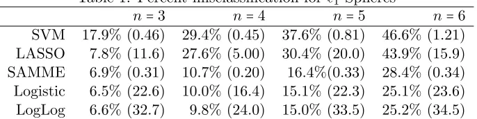
We compared 5 algorithms – the SAMME, our algorithm with the logistic and loglog losses, the SVM and the LASSO logistic regression algorithm. Each simulation, 3200 ob-servations were generated, 200 of which were used for training and 3000 were left out for testing purposes. We performed in total of 500 simulation for each scenario. The results are summarized in the tables 1 and 2 below:

Table 1: Percent misclassification for `1 Spheres

n=3 n=4 n=5 n=6

SVM 17.9% (0.46) 29.4% (0.45) 37.6% (0.81) 46.6% (1.21) LASSO 7.8% (11.6) 27.6% (5.00) 30.4% (20.0) 43.9% (15.9) SAMME 6.9% (0.31) 10.7% (0.20) 16.4%(0.33) 28.4% (0.34) Logistic 6.5% (22.6) 10.0% (16.4) 15.1% (22.3) 25.1% (23.6) LogLog 6.6% (32.7) 9.8% (24.0) 15.0% (33.5) 25.2% (34.5)

Table 2: Percent misclassification for `2 Spheres

n=3 n=4 n=5 n=6

SVM 17.0% (0.44) 28.0% (0.78) 36.6% (0.83) 44.1% (1.15) LASSO 8.7% (11.8) 26.7% (5.70) 31.9% (19.7) 45.0% (14.6) SAMME 8.2% (0.33) 12.9% (0.46) 19.7% (0.30) 28.9% (0.29) Logistic 7.5% (23.4) 11.7% (25.3) 17.3% (24.6) 25.4% (23.5) LogLog 7.7% (33.7) 11.5% (35.6) 17.9% (35.7) 25.8% (35.7)

As we can see our boosting based procedures dominated in all scenarios with the dif-ference becoming more pronounced the more number of classes we have. We observed that our algorithms seem to combine classifiers from the bag more efficiently as compared to the SAMME algorithm in this scenario, especially so when the number of classes was large.

4.2 Experiments with UCI Benchmark Datasets

To present a more comprehensive assessment of our procedure, we analyzed 5 datasets from the UCI machine learning repository. The summaries of the characteristics of the datasets we used can be found in Table 3.

We compare results from SAMME, LogLog and Logistic from our proposed methods, SVM and a multinomial logistic regression (referred to as MLogisticReg). The MLogisticReg

Table 3: Summary of datasets

Dataset Train Set / Test Set Size # Features # Classes

IS Image Segmentation 210/2100 19 7

LED Led Display 200/5000 7 10

RWQ9 Red Wine Quality 700/899 11 4

SE Seeds 100/110 7 3

EC Ecoli 100/236 7 8

was used instead of the LASSO procedure, as these datasets have relatively few features, and the LASSO procedure generally performs worse than the standard. As before all boosting algorithms were ran for 50 iterations.

For the analysis of all 5 datasets, the bag of weak learners we used consisted of decision trees and multinomial logistic regressions with subsampled prefixed number of predictors.

Table 4: Percent misclassifications (run time in seconds)

IS RWQ SE LED EC

SVM 16.19% (0.44) 29.37% (0.28) 8.18% (0.08) 28.64% (1.26) 37.28% (0.27) MLogisticReg 10.57% (0.08) 28.59% (0.09) 5.45% (0.04) 28.34% (0.06) 41.52% (0.04) SAMME 5.09% (0.17) 30.14% (0.74) 4.55% (0.02) 29.36% (0.04) 22.45% (0.02) Logistic 5.00% (13.6) 27.36% (35.3) 3.64% (1.61) 27.02% (1.53) 19.49% (1.22) LogLog 4.95% (16.9) 28.36% (48.8) 3.64% (1.30) 27.00% (2.01) 19.49% (1.45)

We observe that in nearly all cases the newly suggested procedure performed better than the SAMME procedure, which typically converged too fast failing to include enough classifiers. The misclassifications rates of both the Logistic and LogLog based boosting algorithms were also better compared to the SVM and logistic regression in all 4 datasets.

4.3 Summary of Simulation Results and Benchmark Data Analyses

The results provided above demonstrate that the suggested algorithms can be used in suc-cessfully practice, and can outperform existing algorithms in many cases. The proposed boosting algorithm with LogLog loss appears to perform well across all settings considered with respect to classification accuracy. The robustness and gained accuracy of our proposed procedures come at the price of being more computationally intensive than the competi-tors. The slow speed is mostly due to the optimization with respect toβ (see Algorithm 1) required at each iteration for each classifier in the bag. The SAMME algorithm avoids this search as an explicit solution to its corresponding optimization problem exists.

if one opts for sampling not too many classifiers. A relaxation of the procedure might be warranted in cases where a lot of classifiers will be used, and such relaxed algorithms are left for future work.

4.4 Application to an EMR Study of Diabetic Neuropathy

To illustrate our proposed generic boosting algorithm and demonstrate the advantage of having multiple losses, we apply our procedures to an electronic medical record (EMR) study, conducted at the Partners Healthcare, aiming to identify patients with different sub-types of diabetic neuropathy. Diabetic neuropathy (DN), a serious complication of diabetes, is the most common neuropathy in industrialized countries with an estimate of about 20-30 million people affected by symptomatic DN worldwide (Said, 2007). Increasing rates of obesity and type 2 diabetes could potentially double the number of affected individuals by the year 2030. The prevalence of DN also increases with time and poor glycemic control (Martin et al., 2006). Although many types of neuropathy can be associated with diabetes, the most common type is diabetic polyneuropathy and pain can develop as a symptom of di-abetic polyneuropathy (Thomas and Eliasson, 1984; Galer et al., 2000). Pain in the feet and legs was reported to occur in 11.6% of insulin dependent diabetics and 32.1% of noninsulin dependent diabetics (Ziegler et al., 1992). Unfortunately, risk factors for developing painful diabetic neuropathy (pDN) are generally poorly understood. pDN has been reported as more prevalent in patients with type 2 diabetes and women (Abbott et al., 2011). Prior studies have also reported an association between family history and pDN, suggesting a potential genetic predisposition to pDN (Galer et al., 2000). To enable a genetic study of pDN and non-painful DN (npDN), an EMR study was performed to identify patients with these two subtypes of DN by investigators from the informatics for integrating biology to the bedside (i2b2), a National Center for Biomedical Computing based at Partners HealthCare (Murphy et al., 2006, 2010).

To identify such patients, we created a datamart compromising 20,000 patients in the Partners Healthcare with relevant ICD9 (International Classification of Diseases, version 9) codes. Two sources of information were utilized to classify patients’ DN status and subtypes: (i) structured clinical data searchable in the EMR such as ICD9 codes; and (ii) variable identified using natural language processing (NLP) to identify medical concepts in narrative clinical notes. Algorithm development and validation was performed in a training set of 611 patients sampled from the datamart. To obtain the gold standard disease status for these patients, several neurologists performed chart reviews and classified them into no DN, pDN and npDN. The distribution of the classes was 64%,14%,22% respectively. To train the classification algorithms, we included a total of 85 predictors most of which are NLP variables, counting mentions of medical concepts such as “pain”,“hypersensitivity”, and “diabetic neuropathy”.

We trained boosting classification algorithms to classify these 3 disease classes. We used decision stumps as weak learners. They only have two nodes with the first node deciding between class C1 vs C2 and C3 and the other node deciding between C2 vs C3, where

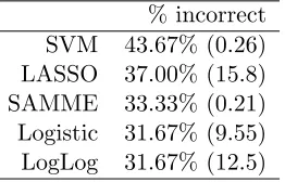
We report the percentage mis-classifications in Table 5. The boosting results show some improvement, as compared to standard methods. We can also see that the generic boosting algorithm performs slightly better than SAMME in this situation with both the logistic and the LogLog losses. It warrants further research whether picking richer tree structures as opposed to using stumps, would yield an even better performance on this dataset.

Table 5: Percent misclassifications (run time in seconds) % incorrect

SVM 43.67% (0.26) LASSO 37.00% (15.8) SAMME 33.33% (0.21) Logistic 31.67% (9.55) LogLog 31.67% (12.5)

5. Discussion

For multi-category classification problems, we described in this paper a class of loss functions that attain FC properties and provided theoretical justifications for how such loss functions can ultimately lead to optimal Bayes classifier. We extended the results to accommodate differential costs in misclassifying different classes. To approximate the minimizer of the empirical losses, we demonstrated that a natural iterative procedure can be used to de-rive generic boosting algorithms for any of the proposed losses. Numerical results suggest that non-convex losses such as LogLog could potentially lead to algorithms with better classification performance. Although the LogLog loss appears to perform well across dif-ferent settings considered in the numerical studies, choosing an optimal loss for a given dataset warrants further research. Our preliminary studies (results not shown) suggest that procedures such as the cross-validation can potentially be used for loss selections.

generic boosting algorithm with coordinate descent, helped us to establish geometric rate of convergence in the convex loss function case. The consistency of the algorithm under conditions such as finite VC dimension of the classifier bag, warrants future research.

Acknowledgments

The authors would like to thank Alexander Rakhlin and three referees for their valuable sug-gestions and feedback, which led to improvements in the present manuscript. This research was partially supported by Research Grants NSF DMS1208771, NIH R01GM113242-01, NIH U54HG007963 and NIH RO1HL089778.

Appendix A. Proofs

Lemma A.1 Assumption (6) implies that the functionφ(g−1(z))is continuously

differen-tiable and convex for all z∈g(S).

Proof [Proof of Lemma A.1] Set z ∶= g(x), z′ ∶= g(x′) in (6). When x, x′ ∈ S we have z, z′

∈g(S) and vice versa. Now (6) can be rewritten as:

φ(g−1(z)) −φ(g−1(z′)) ≥ (z−z′)k(g−1(z′)). (23) Changing the roles of z andz′ _{and using the fact that bothz, z}′

∈g(S) we obtain:

φ(g−1(z′)) −φ(g−1(z)) ≥ (z′−z)k(g−1(z)).

The above two inequalities, combined with the fact thatkandg−1 _{are increasing, give that} for any z≠z′, z, z′∈g(S) we have:

min{k(g−1(z)), k(g−1(z′))} ≤ φ

(g−1(z′)) −φ(g−1(z))

z′_−z ≤max{k(g −1

(z)), k(g−1(z′))}. (24) By the continuity of k and g we have that the composition k(g−1(⋅)) is also continuous. Taking the limitz′

→z in (24) shows that the functionφ(g−1(z))is differentiable on g(S) with a continuous derivative equal to k(g−1_{(z)). Now the convexity of φ(g}−1_{(z)) follows} from (23).

Proof [Proof of Theorem 2.1] To show that Hφ( ̂F_j)w_j = C for someC <0, define Ω= {F= (F1, . . . , Fn) ∶F_j ∈S, j=1, ..., n}, where recall that S= {z∈_R∶k(z) ≤0}. From (6),

n

∑

j=1

φ( ̂F_j)w_j≥

n

∑

j=1

φ(F_j)w_j+

n

∑

j=1

{g( ̂F_j) −g(F_j)}k(F_j)w_j for any F∈Ω. (25)

Since _F̂ _minimizes

∑n_j=1φ(Fj)wj, (25) implies that n

∑

j=1

g(F_j)k(F_j)w_j ≥

n

∑

j=1

For any given constant C < 0, let F̃Cj be the solution to g( ̂Fj)k( ̃FCj)wj = C or equiv-alently _F̃

Cj = k −1

[C /{g( ̂F_j)w_j}]. Obviously F̃_C ∈ Ω for all C < 0. We next show that there exists C₀ < 0 such that ∏n_j=1g( ̃FC0j) = ∏

n j=1g(k

−1

[C₀/{g( ̂F_j)w_j}]) =1. Since g and k are continuous and strictly increasing functions, it suffices to show that ∏n_j=1g( ̃F0j) >1 and ∏n_j=1g( ̃FCj) ≤ 1 for some C. Obviously ∏

n

j=1g( ̃F0j) > 1 since g{k −1

(0)} > g(0) = 1.

Now let C₁ = k(0)max_j{g( ̂F_j)w_j} < 0. Then for all j, C₁/{g( ̂F_j)w_j} ≤ k(0) and thus g(k−1

[C₁/{g( ̂F_j)w_j}]) ≤g(0) = 1. Then by continuity of g and k, there exists C₀ ∈ [C₁,0) such that ∏n_j=1g( ̃F_C0j) = 1. Thus, the constructed F̃_C0 possesses several properties: (i) g( ̂F_j)k( ̃F_C0j)w_j = C₀; (ii)∏n_j=1g( ̃F_C0j) =1; and (iii)k( ̃F_C0j) <0 and henceF̃_C0 ∈Ω. It then follows from the AM-GM inequality that

n

∑

j=1

g( ̃FC0j){−k( ̃FC0j)}wj ≥n

⎡ ⎢ ⎢ ⎢ ⎢ ⎣ n ∏

j=1

g( ̃FC0j){−k( ̃FC0j)}wj

⎤ ⎥ ⎥ ⎥ ⎥ ⎦

n−1

=n ⎡ ⎢ ⎢ ⎢ ⎢ ⎣ n ∏

j=1

g( ̂F_j){−k( ̃FC0j)}wj

⎤ ⎥ ⎥ ⎥ ⎥ ⎦

n−1

= −nC₀,

where we used the fact that∏n_j=1g( ̃F_C0j) = ∏n_j=1g( ̂Fj) =1. This, together with (26), implies that

nC₀ ≥

n

∑

j=1

g( ̃FC0j)k( ̃FC0j)wj ≥ n

∑

j=1

g( ̂F_j)k( ̃FC0j)wj =nC0

and hencenC0= ∑nj=1g( ̃FC0j)k( ̃FC0j)wj. Thus, the equality holds in the AM-GM inequality

above, which also implies thatg( ̃FC0j)k( ̃FC0j)wj = C0. Sinceg( ̂Fj)k( ̃FC0j)wj = C0,k( ̃FC0j) ≠

0 andg is strictly increasing, we have g( ̂F_j) =g( ̃FC0j) and henceF̂j = ̃FC0j. Therefore,

g( ̂F_j)k( ̂F_j)w_j=H_φ( ̂F_j)w_j= C₀. (27) Obviously if Hφ(⋅) is strictly monotone thenF̂_j=H_φ−1(C₀/w_j) which is unique.

Proof [Proof of Proposition 2.2] The function φis strictly decreasing on the set S′ ∶= {z∶

k(z) <0}, as from (6) for anyx<x′, x, x′∈S′ we have:

φ(x) −φ(x′) ≥ (g(x) −g(x′))k(x′) >0.

Furthermore, it follows from Theorem 2.1, that _F̂

j ∈S′ since by (27) k( ̂F_j) <0 for all j. Next we show that ifw>w_j we must haveφ( ̂F_) ≤φ( ̂F_j). This observation follows since:

φ( ̂F_)w_+φ( ̂F_j)w_j≤φ( ̂F_)w_j+φ( ̂F_j)w_,

or elsê_{Fcannot be a minimum of (9), as we can swapF}̂

and F̂j to obtain a strictly smaller value while still satisfying the constraint. Furthermore by Theorem 2.1, w ≠ w_j implies that _F̂

 ≠ ̂F_j because otherwise H_φ( ̂F_) = H_φ( ̂F_j) and hence w_ =w_j by (10). Since φ is strictly decreasing onS′_{it also impliesφ}

( ̂F_) ≠φ( ̂F_j). Hencew_>w_j impliesφ( ̂F_) <φ( ̂F_j). Finally, the last observation gives:

argmin j∈{1,...,n}

φ( ̂F_j) =10argmax

The fact that φis decreasing onS′ _{completes the proof.}

Proof [Proof of Theorem 2.3] To show that a finite minimizer_F̂ _{exists, it suffices to show} thatg( ̂F_j)is finite and bounded away from 0, for j=1, ..., n. To this end, we note that the condition (12) is equivalent to,

lim x↓0

c1φ(g−1(x)) +c2φ(g−1(x−(n−1))) = +∞ for allc₁, c₂>0. (28)

We next show that at the minimizer _F̂_{, m̂ =min}

jg( ̂F_j) =g( ̂F_j∗) is bounded away from 0, where j∗

= argmin_jg( ̂F_j). Since 1= ∏n_j=1g( ̂Fj) ≥g( ̂Fj) ̂m

n−1_{, we have F}̂

j ≤ g−1( ̂m−(n−1)) forj=1, ..., n. Ifφ isdecreasing over_R, then

φ(0)

n

∑

j=1 wj ≥

n

∑

j=1

φ( ̂F_j)w_j =w_j∗φ{g−1( ̂m)} + ∑

j≠j∗

wjφ( ̂F_j)

≥w_j∗φ{g−1( ̂m)} + ∑

j≠j∗

wjφ{g−1( ̂m−(n−1))}.

From (28) with c1 = w_j∗ and c₂ = ∑j≠j∗wj, we conclude that m̂ must be bounded away from 0 since ∑n_j=1φ( ̂Fj)wj→ ∞ if m̂ →0. Thus, there exists m₀>0 such that m̂ ≥m₀ and consequently

0<m₀≤g( ̂F_j) ≤m₀−(n−1)< ∞, j=1, ..., n.

Now, ifφis not decreasing on the wholeR, then there must existF∗< ∞such thatk(F∗) =0 sinceφis strictly decreasing on S′

= {z∶k(z) <0}. Now we show that _F̂ _{∈ Ω ≡ {F = (F}

1, . . . , Fn) ∶ F_j ∈ S, j = 1, . . . , n} as defined in Theorem 2.1. To this end, we note that φ is strictly decreasing on S′ _and

(−∞,0] ⊂ S′. We next argue by contradiction that _F̂

j ∈ S or equivalently F̂_j ≤ F∗ for all j. For any F > F∗, φ(F) −φ(F∗) ≥ {g(F) −g(F∗)}k(F∗) = 0 by (6). Let A = {j ∶ ̂F_j > F∗} and

̂ F∗

j =1(j∈ A)F∗+1(j∉ A) ̂Fj. IfAis not an empty set, then∑n_j=1φ( ̂F_j∗)w_j ≤ ∑n_j=1φ( ̂Fj)wj and ∏n_j=1g( ̂F_j∗) < 1. Since g(F∗) > 1, there must exist some F̂_j∗∗ with F∗ ≥ ̂F_j∗∗ ≥ ̂F_j for j∉ A and F̂_j∗∗=F∗ forj∈ A such that ∏n_j=1g( ̂F_j∗∗) =1 and F∗≥ ̂F_j∗∗> ̂F_j for somej∉ A. Since φ is strictly decreasing on S, ∑n_j=1φ( ̂F_j∗∗)wj < ∑nj=1φ( ̂F

∗

j)wj ≤ ∑nj=1φ( ̂Fj)wj, which contradicts that _F̂ _{is the minimum. Therefore, F}̂_∈Ω.

Hence _F̂

j ≤F∗ andg( ̂F_j) ≤g(F∗) =m₁∈ (0,∞). On the other hand, since∏n_j=1g( ̂Fj) = 1, we haveg( ̂F_j) ≥m₁−(n−1) and thus g( ̂F_j)is also bounded away from 0 and finite.

Remark A.1 As a useful remark we mention that the same argument shows that given any finite vector _F̂_{, the vectors F with ∑}

jφ(Fj)wj ≤ ∑jφ( ̂Fj)wj are located on a compact

set (provided that _F̂

j<F∗ for allj in the second case).

Lemma A.2 Any loss function φ satisfying (6) with g = exp, and either i. or ii. from

Theorem 2.3 is classification calibrated in the two class case.

Remark A.2 Recall that a loss functionφis classification calibrated in the two class case if, for any point w1+w₂=1 withw₁≠ 1₂ and w₁, w₂>0, we have:

inf x∈R

(w₁φ(x) +w₂φ(−x)) > inf

x∶x(2w1−1)≤0

(w₁φ(x) +w₂φ(−x)).

Proof [Proof of Lemma A.2] Denote the two (distinct) class probabilities withw1+w₂=1. Without loss of generality we distinguish two cases: w1 >w₂ >0 and w₁ =1, w₂ =0. First, consider the case when w1 >w₂ >0. Since the conditions of Theorem 2.3 hold, we know that the optimization problem (9) has a minimum, and hence by Proposition 2.2 we have that argmax_j∈{1,2}

̂

Fj ⊆ {1}. Hence it follows that F̂₁ > 0,F̂₂ < 0 at the minimum. This implies that inequality in Remark A.2 is strict.

Next assume that w1 =1, w₂ =0. This case is not covered by our results as we assume that the probabilities are bounded away from 0. As we argued earlierφis strictly decreasing on the setS′ _{and by assumption(−∞,0}

] ⊊S′. Thus by:

̂

F=argmin_F∶F

1+F2=0w1φ(F1) +w2φ(F2) =argminF∶F1+F2=0φ(F1), we must have_F̂

1>0 and hence φ(0) >φ( ̂F₁). This finishes the proof.

Lemma A.3 LetF(m)_{be defined as in iteration (16) starting fromF}(0)

=0. Then we must

have F(m)

∈Ω for allm, where Ω= {F= (F₁, . . . , F_n) ∶F_j∈S, j=1, ..., n}.

Proof [Proof of Lemma A.3] If S = _R there is nothing to prove. Assume that there exists F∗

∈ _R such that k(F∗) = 0. We show the statement by induction. By definition

F(0)

∈ Ω. Assume that F(m−1) ∈ Ω for some m ≥ 1. We now show that F(m) ∈ Ω. To arrive at a contradiction, assume the contrary. Let A = {j ∶ F_j(m) > F∗} ≠ ∅. Define

F∗(m)

j =1(j ∈ A)F (m−1)

j +1(j ∉ A)F (m)

j . Since F (m−1)

∈Ω, it follows that F∗(m) ∈Ω and ∏n_j=1g(F

∗(m)

j ) <1. More importantly, observe that for allj∈ A we have:

0= (g(F_j(m−1)) −g(F_j∗(m)))k(F_j∗(m))w_j > (g(F_j(m−1)) −g(F_j(m)))k(F_j(m))w_j, asg(F(m−1)

j ) ≤g(F ∗

) <g(F_j(m)) and k(F_j(m)) >k(F∗) =0, and hence:

n

∑

j=1

(g(F(m−1)

j ) −g(F ∗(m)

j ))k(F

∗(m) j )wj>

n

∑

j=1

(g(F(m−1)

j ) −g(F (m)

j ))k(F

(m) j )wj.

Define the index set B = {j∶F_j∗(m)<F_j(m−1)}. Since ∏n_j=1g(F∗(_j m)) <1 andF(m−1)∈Ω it follows thatB is not empty andA ∩ B = ∅. Next for λ∈ [0,1]define for allj:

F∗(m),λ

j ∶= [1(j∈ A) +1(j∉ A)1(j∉ B)]F ∗(m)

j +1(j∈ B)((1−λ)F ∗(m) j +λF

Note that when λ=0, we have F_j∗(m),0 ≡F_j∗(m). Now we show that for any λ∈ [0,1] the following inequality holds:

n

∑

j=1

(g(F_j(m−1)) −g(F_j∗(m),λ))k(F_j∗(m),λ)w_j ≥

n

∑

j=1

(g(F_j(m−1)) −g(F_j∗(m)))k(F_j∗(m))w_j. (29)

For any λ ∈ (0,1]: F_j∗(m),λ ≠ F_j∗(m),λ iff j ∈ B. Next note that for any j the function

(g(F(m−1)

j ) −g(x))k(x)wj is an increasing function for x≤F (m−1)

j . The last two observa-tions imply (29). Finally since ∏n_j=1g(F

∗(m),0

j ) = ∏

n j=1g(F

∗(m)

j ) <1 and ∏n_j=1g(F ∗(m),1

j ) ≥

∏_jn₌₁g(F_j(m−1)) =1, by the continuity ofgthere exists aλ∈ (0,1]such that∏n_j=1g(F_j∗(m),λ) = 1. These facts and inequality (29) imply thatF(m)_{would not be a maximum in the iteration} which is a contradiction.

Proof [Proof of Theorem 3.1] By construction we have that on themth iteration the value

F(m)_satisfies

∏m_j=1g(F_j(m)) =1, and Lemma A.3 guarantees thatF(m)∈Ω for allm. Hence, sinceF(m)

j are viable values forF (m+1)

j , the iteration also guarantees that:

n

∑

j=1

{φ(F_j(m)) −φ(F_j(m+1))}w_j≥

n

∑

j=1

{g(F_j(m)) −g(F_j(m+1))}k(F_j(m+1))w_j ≥0.

Now, from Remark A.1, F_j(m+1) lie on a compact set for all j, since for our starting point we have F(0)

j ≡0 ∈Ω. Therefore there must exist a subsequence {m`, `= 1, ...} such that F(m`) _{converges coordinate-wise on this subsequence, and denote with F}∗ _{its limit.}

The functionφis continuous and hence we have that∑n_j=1φ(F_j(m`))w<sub>j</sub>−∑n<sub>j</sub>=1φ(F (m`+1) j )wj → 0. However by the construction of our iteration, the sequences ∑n_j=1φ(F

(m`+1)

j )wj are decreasing for all `. Therefore we have that: ∑n_j=1φ(F

(m)

j )wj − ∑n_j=1φ(F (m+1)

j )wj → 0 holds for all m, not only on the subsequence. But this implies that ∑n_j=1(g(F_j(m)) − g(F(m+1)

j ))k(F

(m+1)

j )wj → 0, which again by the construction is non-negative for all m. Takem`in place ofmin the limit above, and letLbe the set of all limit points lim`→∞F

(m`+1)_. By our construction we have the following inequality holding for any pointFl∈L:

0=

n

∑

j=1 {g(F∗

j) −g(F_jl)}k(F_jl)w_j≥

n

∑

j=1 {g(F∗

j) −g(F_j)}k(F_j)w_j, (30)

for any F∈ Ω with ∏n_j=1g(F_j) =1. Just as in the proof of Theorem 2.1 select ̃F so that g(F_j∗)k( ̃F_j)w_j = C for allj for someC <0. By the AM-GM inequality we get:

n

∑

j=1

g( ̃Fj){−k( ̃Fj)}wj≥n ⎡ ⎢ ⎢ ⎢ ⎢ ⎣ n ∏

j=1

g( ̃Fj){−k( ̃Fj)}wj

⎤ ⎥ ⎥ ⎥ ⎥ ⎦

n−1

=n ⎡ ⎢ ⎢ ⎢ ⎢ ⎣ n ∏

j=1 g(F∗

j){−k( ̃Fj)}wj

⎤ ⎥ ⎥ ⎥ ⎥ ⎦

n−1

=

n

∑

j=1

Now by (30) it follows that equality must be achieved in the preceding display, which implies thatg(F_j∗)k( ̃F_j)w_j = C =g( ̃F_j)k( ̃F_j)w_jand yieldsF̃_j =F_j∗for allj. Henceg(F_j∗)k(F_j∗)w_j = C for all j.

Thus we showed that on subsequences the iteration converges to points satisfying the equality described above. We are left to show, that all these subsequences converge to the same point. Next, take equation (30). By what we showed it follows that for any Fl∈L, we have thatg(F_jl)k(F_jl)wj = Cl for someCl<0. Then we have:

n

∑

j=1

g(F_j∗){−k(F_jl)}w_j ≥n ⎡ ⎢ ⎢ ⎢ ⎢ ⎣ n ∏

j=1

g(F_j∗){−k(F_jl)}w_j ⎤ ⎥ ⎥ ⎥ ⎥ ⎦

n−1

=n ⎡ ⎢ ⎢ ⎢ ⎢ ⎣ n ∏

j=1

g(F_jl){−k(F_jl)}w_j ⎤ ⎥ ⎥ ⎥ ⎥ ⎦

n−1

=

n

∑

j=1

g(F_jl){−k(F_jl)}w_j= −nCl.

Equation (30) implies that the above inequality is in fact equality which shows that:

g(F∗ j)k(F

l

j) =g(F l j)k(F

l

j) for all j.

Thus since k(F_jl) ≠ 0 (recall that all values on the iteration F(m) ∈ Ω) we conclude that g(F_j∗) =g(F_jl), and henceF∗=Fl. This shows that for any converging subsequencem<sub>`</sub> the limiting value coincides with that of the sequence m`+1, which finishes our proof.

Proof [Proof of Proposition 3.2.] It is sufficient to show that for allF∈ G∗ we have:

N

∑

i=1

YT_CiF(X_i)φ˙(Y_CT iF

(∞)

(X_i)) ≥0.

The condition above is sufficient, because of the looping closure ofG. Writing the inequality for all “looped” versions ofFand noting that they sum up to 0, gives us that the inequality is in fact an equality.

Note that with each iteration (18), we decrease the value of the target function. This can be seen by the following inequality:

N

∑

i=1 φ(Y_CT

iF

(m−1)

(X_i))−

N

∑

i=1 φ(Y_CT

iF

(m)

(X_i)) ≥

N

∑

i=1

[exp(−βY_CT

iF(Xi))−1]φ˙(Y

T CiF

(m)

(X_i)) ≥0,

whereF(m)

=F(m−1)+βF. As a remark, the inequality in the preceding display holds, since φis decreasing and thus by (6) we have S=_R.

Take a limiting point11 F(∞) _{of iteration (18), where it is possible having coordinates} of F(∞)

(X_i) equal to ±∞ for some i. Since φ is bounded from below, by our previous observation we have that for anyβ≥0 and F∈ G∗:

N

∑

i=1 φ(Y_CT

iF

(∞)

(X_i)) −

N

∑

i=1 φ(Y_CT

iF

(∞)

(X_i) +βY_CT

iF(Xi)) ≤0.

LetA = {i∶ ∣YT_C iF

(∞)

(X_i)∣ ≠ ∞}. Then the latter inequality also implies that: ∑

i∈A φ(Y_CT

iF

(∞)

(X_i)) − ∑

i∈A φ(YT_C

iF

(∞)

(X_i) +βYT_C

iF(Xi)) ≤0.

12

Applying inequality (6) the above implies:

∑

i∈A

[exp(−βYT_C

iF(Xi)) −1]

˙ φ(Y_CT

iF

(∞)

(X_i) +βYT_C

iF(Xi)) ≤0,

and after a Taylor expansion of the exponent, and division byβ ≥0 we get:

∑

i∈A −YT_C

iF(Xi)

˙ φ(YT_C

iF

(∞) (X_i)) + ∑

i∈A −YT_C

iF(Xi)[

˙ φ(Y_CT

iF

(∞)

(X_i) +βY_CT

iF(Xi)) −

˙ φ(Y_CT

iF

(∞) (X_i))] +O(β) ∑

i∈A ˙ φ(Y_CT

iF

(∞)

(X_i) +βY_CT

iF(Xi)) ≤0.

Lettingβ →0, by the continuity of ˙φ we get:

∑

i∈A

YT_CiF(X_i)φ˙(Y_CT iF

(∞)

(X_i)) ≥0. (31)

Next we argue that ˙φ(+∞) =lim_x→+∞φ˙(x) =0. As stated in the main text ˙φ(x) =k(x)ex. Let K=inf_x∈_Rφ(x). For any ε>0, take a pointx

′ _{such that φ}

(x′) −K ≤ε. Then for any x∈_R, by (6):

ε≥φ(x′) −φ(x) ≥ (ex ′

−ex)k(x),

and thus ε−ex ′

k(x) ≥ −φ˙(x) ≥0. Taking the limit x→ +∞ and letting ε→0 shows that ˙

φ(+∞) =0.

Now consider two cases forφ. Suppose thatφis unbounded from above. We argue that

Y_CT

iF

(∞)

(X_i) ≠ −∞ for all i. Since we start form the point 0, and as we argued we are decreasing the target function we have that:

N φ(0) ≥

N

∑

i=1 φ(Y_CT

iF

(∞)

(X_i)) ≥max

i φ(Y T CiF

(∞)

(X_i)) + (N−1)K,

and hence maxiφ(Y_CT iF

(∞)

(X_i)) ≤N φ(0) − (N−1)K. Sinceφis decreasing and unbounded from above it follows thatYT_CiF(∞)

(X_i) ≠ −∞for all i. In the second case suppose thatφ is bounded from above, and let M =sup_x∈

Rφ(x). We show that ˙φ(−∞) =0. For anyε>0

takex so that ε≥M−φ(x). Applying (6) for anyx′∈_Ryields:

ε≥φ(x′) −φ(x) ≥ (ex ′

−ex)k(x).

This givesε−ex ′

k(x) ≥ −φ˙(x) ≥0. Takingx′→ −∞ gives thatε≥ −φ˙(x) ≥0 for any x such that ε≥ M −φ(x). Since φ is decreasing we are allowed to take the limit x → −∞, and

12. Observe that sinceφis bounded from below the values ofφat infinite points of the iteration i.e. φ(±∞)