Greedy Sparsity-Constrained Optimization
Sohail Bahmani [email protected]
Department of Electrical and Computer Engineering Carnegie Mellon University
5000 Forbes Avenue Pittsburgh, PA 15213, USA
Bhiksha Raj [email protected]
Language Technologies Institute Carnegie Mellon University 5000 Forbes Avenue Pittsburgh, PA 15213, USA
Petros T. Boufounos [email protected]
Mitsubishi Electric Research Laboratories 201 Broadway
Boston, MA 02139, USA
Editor:Francis Bach
Abstract
Sparsity-constrained optimization has wide applicability in machine learning, statistics, and signal processing problems such as feature selection and Compressed Sensing. A vast body of work has studied the sparsity-constrained optimization from theoretical, algorithmic, and application aspects in the context of sparse estimation in linear models where the fidelity of the estimate is measured by the squared error. In contrast, relatively less effort has been made in the study of sparsity-constrained optimization in cases where nonlinear models are involved or the cost function is not quadratic. In this paper we propose a greedy algorithm, Gradient Support Pursuit (GraSP), to approximate sparse minima of cost functions of arbitrary form. Should a cost function have a Stable Restricted Hessian (SRH) or a Stable Restricted Linearization (SRL), both of which are introduced in this paper, our algorithm is guaranteed to produce a sparse vector within a bounded distance from the true sparse optimum. Our approach generalizes known results for quadratic cost functions that arise in sparse linear regression and Compressed Sensing. We also evaluate the performance of GraSP through numerical simulations on synthetic and real data, where the algorithm is employed for sparse logistic regression with and withoutℓ2-regularization.
Keywords: sparsity, optimization, compressed sensing, greedy algorithm
1. Introduction
exhibit significant structure, which sparsity models are often able to capture. This structure can be exploited for robust regression and hypothesis testing, model reduction and variable selection, and
more efficient signal acquisition inunderdeterminedregimes. Estimation of parameters with sparse
structure is usually cast as an optimization problem, formulated according to specific application requirements. Developing techniques that are robust and computationally tractable to solve these optimization problems, even only approximately, is therefore critical.
In particular, theoretical and application aspects of sparse estimation in linear models have been studied extensively in areas such as signal processing, machine learning, and statistics. However, sparse estimation in problems where nonlinear models are involved have received comparatively
little attention. Most of the work in this area extend the use of theℓ1-norm as a regularizer,
effec-tive to induce sparse solutions in linear regression, to problems with nonlinear models (see, e.g., Bunea, 2008; van de Geer, 2008; Kakade et al., 2010; Negahban et al., 2009). As a special case,
logistic regression withℓ1and elastic net regularization are studied by Bunea (2008). Furthermore,
Kakade et al. (2010) have studied the accuracy of sparse estimation throughℓ1-regularization for the
exponential family distributions. A more general frame of study is proposed and analyzed by Negah-ban et al. (2009) where regularization with “decomposable” norms is considered in M-estimation problems. To provide the accuracy guarantees, these works generalize the Restricted Eigenvalue condition (Bickel et al., 2009) to ensure that the loss function is strongly convex over a restriction of its domain. We would like to emphasize that these sufficient conditions generally hold with proper constants and with high probability only if one assumes that the true parameter is bounded. This fact is more apparent in some of the mentioned work (e.g., Bunea, 2008; Kakade et al., 2010), while in some others (e.g., Negahban et al., 2009) the assumption is not explicitly stated. We will elaborate on this matter in Section 2. Tewari et al. (2011) also proposed a coordinate-descent type algorithm for minimization of a convex and smooth objective over the convex signal/parameter models
intro-duced in Chandrasekaran et al. (2012). This formulation includes theℓ1-constrained minimization
as a special case, and the algorithm is shown to converge to the minimum in objective value similar to the standard results in convex optimization.
This paper presents an extended version with improved guarantees of our prior work in Bah-mani et al. (2011), where we proposed a greedy algorithm, the Gradient Support Pursuit (GraSP), for sparse estimation problems that arise in applications with general nonlinear models. We prove
the accuracy of GraSP for a class of cost functions that have aStable Restricted Hessian(SRH). The
SRH, introduced in Bahmani et al. (2011), characterizes the functions whose restriction to sparse canonical subspaces have well-conditioned Hessian matrices. Similarly, we analyze the GraSP
algo-rithm for non-smooth functions that have aStable Restricted Linearization(SRL), a property
intro-duced in this paper, analogous to SRH. The analysis and the guarantees for smooth and non-smooth cost functions are similar, except for less stringent conditions derived for smooth cost functions due to properties of symmetric Hessian matrices. We also prove that the SRH holds for the case of the
ℓ2-penalized logistic loss function.
1.1 Notation
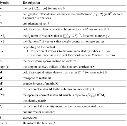
In the remainder of this paper we use the notation listed in Table 1.
1.2 Paper Outline
In Section 2 we provide a background on sparse parameter estimation which serves as an overview of prior work. In Section 3 we state the general formulation of the problem and present our al-gorithm. Conditions that characterize the cost functions and the main accuracy guarantees of our algorithm are provided in Section 3 as well. The guarantees of the algorithm are proved in
Appen-dices A and B. As an example where our algorithm can be applied,ℓ2-regularized logistic regression
is studied in Section 4. Some experimental results for logistic regression with sparsity constraints are presented in Section 5. Finally, Section 6 discusses the results and concludes.
2. Background
We first briefly review sparse estimation problems studied in the literature.
2.1 Sparse Linear Regression and Compressed Sensing
The special case of sparse estimation in linear models has gained significant attention under the title of Compressed Sensing (CS) (Donoho, 2006). In standard CS problems the aim is to estimate
a sparse vectorx⋆from noisy linear measurementsy=Ax⋆+e, whereAis a knownn×p
mea-surement matrix withn≪pandeis the additive measurement noise. To find the sparsest estimate
in thisunderdeterminedproblem that is consistent with the measurementsyone needs to solve the
optimization problem
b
x=arg min
x kxk0 s.t. ky−Axk2≤ε, (1)
whereεis a given upper bound forkek2 (Cand`es et al., 2006). In the absence of noise (i.e., when
ε=0), ifx⋆iss-sparse (i.e., it has at mostsnonzero entries) one merely needs every 2scolumns of
Ato be linearly independent to guarantee exact recovery (Donoho and Elad, 2003). Unfortunately,
the ideal solver (1) is computationally NP-hard in general (Natarajan, 1995) and one must seek approximate solvers instead.
It is shown in Cand`es et al. (2006) that under certain conditions, minimizing the ℓ1-norm as
Symbol Description
[n] the set{1,2, . . . ,n}for anyn∈N
I
calligraphic letters denote sets unless stated otherwise (e.g.,N
µ,σ2denotes
a normal distribution)
I
c complement of setI
v bold face small letters denote column vectors inRbfor someb∈N
kvkq theℓq-norm of vectorv, that is ∑b
i=1|vi|q
1/q
, for a real numberq≥1
kvk0 the “ℓ0-norm” of vectorvthat merely counts its nonzero entries
v|I
depending on the context
1. restriction of vectorvto the rows indicated by indices in
I
, or2. a vector that equalsvexcept for coordinates in
I
cwhere it is zerovr the bestr-term approximation of vectorv
supp(v) the support set (i.e., indices of the non-zero entries) ofv
M bold face capital letters denote matrices inRa×bfor somea,b∈N
MT transpose of matrixM
M† pseudo-inverse of matrixM
MI restriction of matrixMto the columns enumerated by
I
kMk the operator norm of matrixMwhich is equal topλmax(MTM)
I the identity matrix
PI restriction of the identity matrix to the columns indicated by
I
1 column vector of all ones
E[·] expectation
Hf(·) Hessian of the function f
basically returns the solution to the convex optimization problem
b
x=arg min
x kxk1 s.t. ky−Axk2≤ε, (2)
The required conditions for approximate equivalence of (1) and (2), however, generally hold only if
measurements are collected at a higher rate. Ideally, one merely needsn=O(s)measurements to
estimatex⋆, butn=O(slogps)measurements are necessary for the accuracy of (2) to be guaranteed.
The convex program (2) can be solved in polynomial time using interior point methods. How-ever, these methods do not scale well as the size of the problem grows. Therefore, several first-order convex optimization methods are developed and analyzed as more efficient alternatives (see, e.g., Beck and Teboulle, 2009; Agarwal et al., 2010). Another category of low-complexity algorithms in
CS are the non-convexgreedy pursuitsincluding Orthogonal Matching Pursuit (OMP) (Pati et al.,
1993; Tropp and Gilbert, 2007), Compressive Sampling Matching Pursuit (CoSaMP) (Needell and Tropp, 2009), Iterative Hard Thresholding (IHT) (Blumensath and Davies, 2009), and Subspace Pursuit (Dai and Milenkovic, 2009) to name a few. These greedy algorithms implicitly approximate
the solution to theℓ0-constrained least squares problem
bx=arg min
x
1
2ky−Axk
2
2 s.t. kxk0≤s. (3)
The main theme of these iterative algorithms is to use the residual error from the previous iteration to successively approximate the position of non-zero entries and estimate their values. These algo-rithms have shown to exhibit accuracy guarantees similar to those of convex optimization methods, though with more stringent requirements.
As mentioned above, to guarantee accuracy of the CS algorithms the measurement matrix should
meet certain conditions such asincoherence(Donoho and Huo, 2001), Restricted Isometry Property
(RIP) (Cand`es et al., 2006), Nullspace Property (Cohen et al., 2009), etc. Among these conditions RIP is the most commonly used and the best understood condition.
MatrixAis said to satisfy the RIP of orderk—in its symmetric form—with constantδk, ifδk<1
is the smallest number that
(1−δk)kxk22≤ kAxk 2
2≤(1+δk)kxk22
holds for all k-sparse vectorsx. Several CS algorithms are shown to produce accurate solutions
provided that the measurement matrix has a sufficiently small RIP constant of orderckwithcbeing
a small integer. For example, solving (2) is guaranteed to yield an accurate estimate ofs-sparse
x⋆ifδ2s<
√
2−1 (Cand`es, 2008). Interested readers can find the best known RIP-based accuracy
guarantees for some of the CS algorithms in Foucart (2012).
2.2 Beyond Linear Models
The existing studies on this subject are mostly in the context of statistical estimation. The
majority of these studies consider the cost function to be convex everywhere and rely on the ℓ1
-regularization as the means to induce sparsity in the solution. For example, Kakade et al. (2010) have shown that for the exponential family of distributions maximum likelihood estimation with
ℓ1-regularization yields accurate estimates of the underlying sparse parameter. Furthermore,
Negah-ban et al. have developed a unifying framework for analyzing statistical accuracy ofM-estimators
regularized by “decomposable” norms in (Negahban et al., 2009). In particular, in their workℓ1
-regularization is applied to Generalized Linear Models (GLM) (Dobson and Barnett, 2008) and shown to guarantee a bounded distance between the estimate and the true statistical parameter. To
establish this error bound they introduced the notion ofRestricted Strong Convexity(RSC), which
basically requires a lower bound on the curvature of the cost function around the true parameter in a restricted set of directions. The achieved error bound in this framework is inversely proportional to this curvature bound. Furthermore, Agarwal et al. (2010) have studied Projected Gradient Descent
as a method to solve ℓ1-constrained optimization problems and established accuracy guarantees
using a slightly different notion of RSC andRestricted Smoothness(RSM).
Note that the guarantees provided for majority of theℓ1-regularization algorithms presume that
the true parameter is bounded, albeit implicitly. For instance, the error bound forℓ1-regularized
lo-gistic regression is recognized by Bunea (2008) to be dependent on the true parameter (Bunea, 2008, Assumption A, Theorem 2.4, and the remark that succeeds them). Moreover, the result proposed by Kakade et al. (2010) implicitly requires the true parameter to have a sufficiently short length to allow the choice of the desirable regularization coefficient (Kakade et al., 2010, Theorems 4.2 and 4.5). Negahban et al. (2009) also assume that the true parameter is inside the unit ball to establish
the required condition for their analysis ofℓ1-regularized GLM, although this restriction is not
ex-plicitly stated (see the longer version of Negahban et al., 2009, p. 37). We can better understand why restricting the length of the true parameter may generally be inevitable by viewing these esti-mation problems from the perspective of empirical processes and their convergence. The empirical processes, including those considered in the studies mentioned above, are generally good approxi-mations of their corresponding expected process (see Vapnik, 1998, chap. 5 and van de Geer, 2000). Therefore, if the expected process is not strongly convex over an unbounded, but perhaps otherwise restricted, set the corresponding empirical process cannot be strongly convex over the same set. This reasoning applies in many cases including the studies mentioned above, where it would be impossible to achieve the desired restricted strong convexity properties—with high probability—if the true parameter is allowed to be unbounded.
Furthermore, the methods that rely on theℓ1-norm are known to result in sparse solutions, but,
as mentioned in Kakade et al. (2010), the sparsity of these solutions is not known to be optimal in general. One can intuit this fact from definitions of RSC and RSM. These two properties bound the curvature of the function from below and above in a restricted set of directions around the true optimum. For quadratic cost functions, such as squared error, these curvature bounds are absolute constants. As stated before, for more general cost functions such as the loss functions in GLMs, however, these constants will depend on the location of the true optimum. Consequently, depending on the location of the true optimum these error bounds could be extremely large, albeit finite. When
error bounds are significantly large, the sparsity of the solution obtained byℓ1-regularization may
not be satisfactory. This motivates investigation of algorithms that do not rely onℓ1-norm to induce
3. Problem Formulation and the GraSP Algorithm
As seen in Section 2.1, in standard CS the squared error f(x) = 12ky−Axk22 is used to measure
fidelity of the estimate. While this is appropriate for a large number of signal acquisition applica-tions, it is not the right cost in other fields. Thus, the significant advances in CS cannot readily be applied in these fields when estimation or prediction of sparse parameters become necessary. In this paper we focus on a generalization of (3) where a generic cost function replaces the squared error.
Specifically, for the cost function f :Rp7→R, it is desirable to approximate
arg min
x f(x) s.t. kxk0≤s. (4)
We propose the Gradient Support Pursuit (GraSP) algorithm, which is inspired by and generalizes the CoSaMP algorithm, to approximate the solution to (4) for a broader class of cost functions.
Of course, even for a simple quadratic objective, (4) can have combinatorial complexity and become NP-hard. However, similar to the results of CS, knowing that the cost function obeys certain properties allows us to obtain accurate estimates through tractable algorithms. To guarantee that GraSP yields accurate solutions and is a tractable algorithm, we also require the cost function to have certain properties that will be described in Section 3.2. These properties are analogous to and generalize the RIP in the standard CS framework. For smooth cost functions we introduce the notion of a Stable Restricted Hessian (SRH) and for non-smooth cost functions we introduce the Stable Restricted Linearization (SRL). Both of these properties basically bound the Bregman divergence of the cost function restricted to sparse canonical subspaces. However, the analysis based on the SRH is facilitated by matrix algebra that results in somewhat less restrictive requirements for the cost function.
3.1 Algorithm Description
Algorithm 1:The GraSP algorithm
input : f(·)ands
output: ˆx
initialize:bx=0
repeat
compute local gradient: z=∇f(bx) identify directions:
Z
=supp(z2s)merge supports:
T
=Z
∪supp(bx)minimize over support: b=arg minf(x) s.t. x|Tc=0
prune estimate:bx=bs
untilhalting condition holds
GraSP is an iterative algorithm, summarized in Algorithm 1, that maintains and updates an
esti-matebxof the sparse optimum at every iteration. The first step in each iteration,z=∇f(bx), evaluates
the gradient of the cost function at the current estimate. For nonsmooth functions, instead of the
gradient we use arestricted subgradient z=∇f(bx) defined in Section 3.2. Then 2s coordinates
of the vectorz that have the largest magnitude are chosen as the directions in which pursuing the
with the support of the current estimate to obtain
T
=Z
∪supp(bx). The combined support is a setof at most 3s indices over which the function f is minimized to produce an intermediate estimate
b=arg minf(x) s.t. x|Tc=0. The estimatebxis then updated as the best s-term approximation of
the intermediate estimate b. The iterations terminate once certain condition, for instance, on the
change of the cost function or the change of the estimated minimum from the previous iteration, holds.
In the special case where the squared error f(x) = 1
2ky−Axk 2
2 is the cost function, GraSP
reduces to CoSaMP. Specifically, the gradient step reduces to the proxy stepz=AT(y−Ax)ˆ and
minimization over the restricted support reduces to the constrained pseudoinverse step b|T =A†Ty,
b|Tc =0in CoSaMP.
VariantsAlthough in this paper we only analyze the standard form of GraSP outlined in Algorithm 1, other variants of the algorithm can also be studied. Below we list some of these variants.
1. Debiasing: In this variant, instead of performing a hard thresholding on the vector b, the
objective is minimized restricted to the support set ofbsto obtain the new iterate:
b
x=arg min
x f(x) s.t. supp(x)⊆supp(bs).
2. Restricted Newton Step: To reduce the computations in each iteration, the minimization that
yieldsb, we can set b|Tc=0and take a restricted Newton step as
b|T =bx|T −κ PTTHf(bx)PT
−1 bx|T ,
where κ>0 is a step-size. Of course, here we are assuming that the restricted Hessian,
PTTHf(bx)PT, is invertible.
3. Restricted Gradient Descent: The minimization step can be relaxed even further by applying
a restricted gradient descent. In this approach, we again setb|Tc=0and
b|T =bx|T −κ ∇f(bx)|T.
Since
T
contains both the support set ofbxand the 2s-largest entries of∇f(bx), it is easy toshow that each iteration of this alternative method is equivalent to a standard gradient descent followed by a hard thresholding. In particular, if the squared error is the cost function as in standard CS, this variant reduces to the IHT algorithm.
3.2 Sparse Reconstruction Conditions
Definition 1(Stable Restricted Hessian). Suppose that f is a twice continuously differentiable
func-tion whose Hessian is denoted byHf(·). Furthermore, let
Ak(x) =sup
n
∆THf(x)∆
|supp(x)∪supp(∆)| ≤k,k∆k2=1o (5) and
Bk(x) =inf
n
∆TH
f(x)∆
|supp(x)∪supp(∆)| ≤k,k∆k2=1
o
, (6)
for allk-sparse vectorsx. Then f is said to have a Stable Restricted Hessian (SRH) with constant
µk, or in shortµk-SRH, if 1≤ABkk((xx))≤µk.
Remark1. Since the Hessian of fis symmetric, an equivalent for Definition 1 is that a twice
contin-uously differentiable function f hasµk-SRH if the condition number ofPKHf(x)PTK is not greater
thanµk for allk-sparse vectorsxand sets
K
⊆[p]with|supp(x)∪K
| ≤k.In the special case when the cost function is the squared error as in (3), we can writeHf(x) =
ATAwhich is constant. The SRH condition then requires
Bkk∆k22≤ kA∆k22≤Akk∆k22
to hold for allk-sparse vectors∆withAk/Bk≤µk. Therefore, in this special case the SRH condition
essentially becomes equivalent to the RIP condition.
Remark2. Note that the functions that satisfy the SRH are convex over canonical sparse subspaces, but they are not necessarily convex everywhere. The following two examples describe some non-convex functions that have SRH.
Example1. Let f(x) =12xTQx, whereQ=2×11T−I. Obviously, we haveHf(x) =Q. Therefore,
(5) and (6) determine the extreme eigenvalues across all of thek×ksymmetric submatrices ofQ.
Note that the diagonal entries ofQare all equal to one, while its off-diagonal entries are all equal to
two. Therefore, for any 1-sparse signaluwe haveuTQu=kuk22, meaning that f hasµ1-SRH with
µ1=1. However, foru= [1,−1,0, . . . ,0]T we haveuTQu<0, which means that the Hessian of f
is not positive semi-definite (i.e., f is not convex).
Example2. Let f(x) =12kxk22+Cx1x2···xk+1where the dimensionality ofxis greater thank. It is
obvious that this function is convex fork-sparse vectors asx1x2···xk+1=0 for anyk-sparse vector.
So we can easily verify that f satisfies SRH of orderk. However, forx1=x2=···=xk+1=tand
xi=0 fori>k+1 the restriction of the Hessian of f to indices in[k+1](i.e.,PT[k+1]Hf(x)P[k+1])
is a matrix with diagonal entries all equal to one and off-diagonal entries all equal toCtk−1. Let
Qdenote this matrix andube a unit-norm vector such thathu,1i=0. Then it is straightforward
to verify thatuTQu=1−Ctk−1, which can be negative for sufficiently large values ofC andt.
Therefore, the Hessian of f is not positive semi-definite everywhere, meaning that f is not convex.
To generalize the notion of SRH to the case of nonsmooth functions, first we define therestricted
subgradientof a function.
Definition 2(Restricted Subgradient). We say vector∇f(x)is a restricted subgradient of f :Rp7→R
at pointxif
f(x+∆)−f(x)≥∇f(x),∆
Remark3. We introduced the notion of restricted subgradient so that the restrictions imposed on f
are as minimal as we need. We acknowledge that the existence of restricted subgradients implies convexity in sparse directions, but it does not imply convexity everywhere.
Remark4. Obviously, if the function f is convex everywhere, then any subgradient of f determines
a restricted subgradient of f as well. In general one may need to invoke the axiom of choice to
define the restricted subgradient.
Remark5. We drop the sparsity level from the notation as it can be understood from the context.
With a slight abuse of terminology we call
Bf x′kx
= f x′−f(x)−∇f(x),x′−x
the restricted Bregman divergence of f :Rp 7→R between pointsx andx′ where ∇f(·) gives a
restricted subgradient of f(·).
Definition 3 (Stable Restricted Linearization). Let x be a k-sparse vector in Rp. For function
f :Rp7→Rwe define the functions
αk(x) =sup
(
1
k∆k22Bf(x+∆kx) |∆6=0 and|supp(x)∪supp(∆)| ≤k
)
and
βk(x) =inf
(
1
k∆k22Bf(x+∆kx) |∆6=0 and |supp(x)∪supp(∆)| ≤k
) .
Then f(·)is said to have a Stable Restricted Linearization with constantµk, orµk-SRL, if βαkk((xx))≤µk
for allk-sparse vectorsx.
Remark6. The SRH and SRL conditions are similar to various forms of the Restricted Strong Con-vexity (RSC) and Restricted Strong Smoothness (RSS) conditions (Negahban et al., 2009; Agarwal et al., 2010; Blumensath, 2010; Jalali et al., 2011; Zhang, 2011) in the sense that they all bound the curvature of the objective function over a restricted set. The SRL condition quantifies the curvature in terms of a (restricted) Bregman divergence similar to RSC and RSS. The quadratic form used in SRH can also be converted to the Bregman divergence form used in RSC and RSS and vice-versa using the mean-value theorem. However, compared to various forms of RSC and RSS conditions SRH and SRL have some important distinctions. The main difference is that the bounds in SRH and SRL conditions are not global constants; only their ratio is required to be bounded globally. Furthermore, unlike the SRH and SRL conditions the variants of RSC and RSS, that are used in convex relaxation methods, are required to hold over a set which is strictly larger than the set of
canonicalk-sparse vectors.
3.3 Main Theorems
Now we can state our main results regarding approximation of
x⋆=arg min f(x)s.t. kxk0≤s, (7)
using the GraSP algorithm.
Theorem 1. Suppose that f is a twice continuously differentiable function that has µ4s-SRH with
µ4s≤1+
√
3
2 . Furthermore, suppose that for someε>0we haveε≤B4s(x)for all4s-sparse vectors
x. Thenbx(i), the estimate at the i-th iteration, satisfies
bx(i)−x⋆
2≤2
−i
kx⋆k2+6+2
√
3
ε k∇f(x
⋆) |Ik2, where
I
is the position of the3s largest entries of∇f(x⋆)in magnitude.Remark 7. Note that this result indicates that∇f(x⋆) determines how accurate the estimate can
be. In particular, if the sparse minimumx⋆ is sufficiently close to an unconstrained minimum of
f then the estimation error floor is negligible because∇f(x⋆)has small magnitude. This result is
analogous to accuracy guarantees for estimation from noisy measurements in CS (Cand`es et al., 2006; Needell and Tropp, 2009).
Remark8. As the derivations required to prove Theorem 1 show, the provided accuracy guarantee
holds for any s-sparse x⋆, even if it does not obey (7). Obviously, for arbitrary choices of x⋆,
∇f(x⋆)|I may have a large norm that cannot be bounded properly which implies large errors. In
statistical estimation problems, often the true parameter that describes the data is chosen as the target
parameter x⋆ rather than the minimizer of the average loss function as in (7). In these problems,
the approximation errork∇f(x⋆)|Ik2has statistical interpretation and can determine the statistical
precision of the problem. This property is easy to verify in linear regression problems. We will also show this for the logistic loss as an example in Section 4.
Nonsmooth cost functions should be treated differently, since we do not have the luxury of working with Hessian matrices for these type of functions. The following theorem provides guar-antees that are similar to those of Theorem 1 for nonsmooth cost functions that satisfy the SRL condition.
Theorem 2. Suppose that f is a function that is not necessarily smooth, but it satisfies µ4s-SRL with
µ4s≤ 3+
√
3
4 . Furthermore, suppose that forβ4s(·)in Definition 3 there exists someε>0such that
β4s(x)≥εholds for all4s-sparse vectorsx. Thenbx(i), the estimate at the i-th iteration, satisfies
bx(i)−x⋆
2≤2−ikx⋆k2+6+2
√
3
ε
∇f(x⋆)
I
2, where
I
is the position of the3s largest entries of∇f(x⋆)in magnitude.Remark9. Should the SRH or SRL conditions hold for the objective function, it is straightforward
to convert thepoint accuracyguarantees of Theorems 1 and 2, into accuracy guarantees in terms of
the objective value. First we can use SRH or SRL to bound the Bregman divergence, or its restricted
version defined above, for pointsbx(i)andx⋆. Then we can obtain a bound for the accuracy of the
4. Example: Sparse Minimization ofℓ2-regularized Logistic Regression
One of the models widely used in machine learning and statistics is the logistic model. In this model
the relation between the data, represented by a random vector a∈Rp, and its associated label,
represented by a random binary variabley∈ {0,1}, is determined by the conditional probability
Pr{y|a;x}= exp(yha,xi)
1+exp(ha,xi), (8)
wherexdenotes a parameter vector. Then, for a set ofnindependently drawn data samples{(ai,yi)}ni=1
the joint likelihood can be written as a function ofx. To find the maximum likelihood estimate one
should maximize this likelihood function, or equivalently minimize the negative log-likelihood, the logistic loss,
g(x) =1
n
n
∑
i=1
log(1+exp(hai,xi))−yihai,xi.
It is well-known thatg(·)is strictly convex for p≤n provided that the associated design matrix,
A= [a1a2. . .an]T, is full-rank. However, in many important applications (e.g., feature selection)
the problem can be underdetermined (i.e., n<p). In these scenarios the logistic loss is merely
convex and it does not have a unique minimum. Furthermore, it is possible, especially in
under-determined problems, that the observed data islinearly separable. In that case one can achieve
arbitrarily small loss values by tending the parameters to infinity along certain directions. To com-pensate for these drawbacks the logistic loss is usually regularized by some penalty term (Hastie et al., 2009; Bunea, 2008).
One of the candidates for the penalty function is the (squared)ℓ2-norm of x(i.e.,kxk22).
Con-sidering a positive penalty coefficientηthe regularized loss is
f(x) =g(x) +η
2kxk
2 2.
For any convexg(·)this regularized loss is guaranteed to beη-strongly convex, thus it has a unique
minimum. Furthermore, the penalty term implicitly bounds the length of the minimizer thereby
resolving the aforementioned problems. Nevertheless, theℓ2penalty does not promote sparse
solu-tions. Therefore, it is often desirable to impose an explicit sparsity constraint, in addition to theℓ2
regularizer.
4.1 Verifying SRH forℓ2-regularized Logistic Loss
It is easy to show that the Hessian of the logistic loss at any pointxis given byHg(x) =41nATΛA,
whereΛ is ann×ndiagonal matrix whose diagonal entries are Λii=sech2 12hai,xiwith sech(·)
denoting the hyperbolic secant function. Note that 04Hg(x)4 41nATA. Therefore, if Hη(x)
denotes the Hessian of theℓ2-regularized logistic loss, we have
∀x,∆ ηk∆k22≤∆TH
η(x)∆≤
1 4nkA∆k
2
2+ηk∆k 2
2. (9)
To verify SRH, the upper and lower bounds achieved atk-sparse vectors∆are of particular interest.
It only remains to find an appropriate upper bound forkA∆k22in terms ofk∆k22. To this end we use
Theorem 3(Matrix Chernoff (Tropp, 2012)). Consider a finite sequence{Mi}of k×k,
indepen-dent, random, self-adjoint matrices that satisfy
Mi<0 and λmax(Mi)≤R almost surely.
Letθmax:=λmax(∑iE[Mi]). Then forτ≥0,
Pr
(
λmax
∑
i
Mi
!
≥(1+τ)θmax )
≤kexp
θmax
R (τ−(1+τ)log(1+τ)
.
As stated before, in a standard logistic model data samples{ai}are supposed to be independent
instances of a random vectora. In order to apply Theorem 3 we need to make the following extra
assumptions:
Assumption. For every
J
⊆[p]with|J
|=k,(i) we havea|J
2
2≤Ralmost surely, and
(ii) none of the matricesPTJEaaTPJ is the zero matrix.
We defineθJmax:=λmax PTJCPJ, whereC=EaaT, and let
θ:= max
J⊆[p],|J|=kθ J
max and eθ:= min
J⊆[p],|J|=kθ J
max.
To simplify the notation henceforth we leth(τ) = (1+τ)log(1+τ)−τ.
Corollary 1. With the above assumptions, if n≥eR
θh(τ) logk+k 1+log
p k
−logεfor someτ>0
andε∈(0,1), then with probability at least1−εtheℓ2-regularized logistic loss has µk-SRH with
µk≤1+14+ητθ.
Proof For any set ofkindices
J
letMJi =ai|J ai|TJ =PTJaiaTiPJ. The independence of the vectorsaiimplies that the matrix
ATJAJ = n
∑
i=1
ai|J ai|TJ
=
n
∑
i=1
MJi
is a sum ofnindependent, random, self-adjoint matrices. Assumption (i) implies thatλmax
MJi=
ai|J
2
2≤Ralmost surely. Furthermore, we have
λmax
n
∑
i=1
EhMJ
i
i!
=λmax
n
∑
i=1
EPTJaiaTiPJ !
=λmax
n
∑
i=1
PTJE
aiaTi
PJ
!
=λmax
n
∑
i=1
PTJCPJ
!
=nλmax PTJCPJ
Hence, for any fixed index set
J
with|J
|=kwe may apply Theorem 3 forMi=MJi,θmax=nθJmax,andτ>0 to obtain
Pr
(
λmax
n
∑
i=1
MJi
!
≥(1+τ)nθJmax
)
≤kexp −nθ
J
maxh(τ)
R !
.
Furthermore, we can write
Prλmax ATJAJ≥(1+τ)nθ =Pr
(
λmax
n
∑
i=1
MJi
!
≥(1+τ)nθ
)
≤Pr
(
λmax
n
∑
i=1
MJi
!
≥(1+τ)nθJmax
)
≤kexp −nθ
J
maxh(τ)
R !
≤kexp −neθh(τ)
R !
. (10)
Note that Assumption (ii) guarantees thateθ>0, and thus the above probability bound will not be
vacuous for sufficiently largen. To ensure a uniform guarantee for all pkpossible choices of
J
wecan use the union bound to obtain
Pr
_
J⊆[p]
|J|=k
λmax ATJAJ≥(1+τ)nθ
≤
∑
J⊆[p]
|J|=k
Prλmax ATJAJ≥(1+τ)nθ
≤k
p k
exp −neθh(τ)
R !
≤kpe k
k
exp −neθh(τ)
R !
=exp logk+k+klogp
k− neθh(τ)
R !
.
Therefore, forε∈(0,1)andn≥R logk+k 1+logpk−logε/eθh(τ)it follows from (9) that
for anyxand anyk-sparse∆,
ηk∆k22≤∆THη(x)∆≤
η+1+τ
4 θ
k∆k22
holds with probability at least 1−ε. Thus, the ℓ2-regularized logistic loss has an SRH constant
Remark10. One implication of this result is that for a regime in whichkand pgrow sufficiently
large while pk remains constant one can achieve small failure rates provided thatn=Ω Rklogkp.
Note that R is deliberately included in the argument of the order function because in general R
depends on k. In other words, the above analysis may require n=Ω k2logpk as the sufficient
number of observations. This bound is a consequence of using Theorem 3, but to the best of our knowledge, other results regarding the extreme eigenvalues of the average of independent random
PSD matrices also yield annof the same order. If matrixAhas certain additional properties (e.g.,
independent and sub-Gaussian entries), however, a better rate ofn=Ω klogpk can be achieved
without using the techniques mentioned above.
Remark11. The analysis provided here is not specific to theℓ2-regularized logistic loss and can be
readily extended to any otherℓ2-regularized GLM loss whose log-partition function has a
Lipschitz-continuous derivative.
4.2 Bounding the Approximation Error
We are going to bound k∇f(x⋆)|Ik2 which controls the approximation error in the statement of
Theorem 1. In the case of case ofℓ2-regularized logistic loss considered in this section we have
∇f(x) =
n
∑
i=1
1
1+exp(−hai,xi)−
yi
ai+ηx.
Denoting 1+exp(−h1 ai,x⋆i)−yibyvifori=1,2, . . . ,nthen we can deduce
k∇f(x⋆)|Ik2=
1
n
n
∑
i=1
viai|I+ηx⋆|I
2
=
1
nA T
Iv+ηx⋆|I
2
≤1nATI
kvk2+ηkx⋆|Ik2
≤√1 nkAIk
s
1
n
n
∑
i=1
v2i +ηkx⋆|Ik2,
where v = [v1v2. . .vn]T. Note that vi’s are n independent copies of the random variable v=
1
1+exp(−ha,x⋆i)−y that is zero-mean and always lie in the interval[−1,1]. Therefore, applying the
Hoeffding’s inequality yields
Pr
(
1
n
n
∑
i=1
v2i ≥(1+c)σ2v
)
whereσ2
v=E
v2is the variance ofv. Furthermore, using the logistic model (8) we can deduce
σ2
v =E
v2
=EEv2|a
=EhEh(y−E[y|a])2|aii
=E[var(y|a)]
=E
1
1+exp(ha,x⋆i)×
exp(ha,x⋆i)
1+exp(ha,x⋆i)
(becausey|a∼Bernoulli as in (8))
=E
1
2+exp(ha,x⋆i) +exp(−ha,x⋆i)
≤14 (because exp(t) +exp(−t)≥2).
Therefore, we have 1n∑ni=1v2i <14 with high probability. As in the previous subsection one can also
bound √1nkAIk=
q 1
nλmax ATIAIusing (10) withk=|
I
|=3s. Hence, with high probability wehave
k∇f(x⋆)|Ik2≤
1 2
q
(1+τ)θ+ηkx⋆k2.
Interestingly, this analysis can also be extended to the GLMs whose log-partition function ψ(·)
obeys 0≤ψ′′(t)≤Cfor alltwithCbeing a positive constant. For these models the approximation
error can be bounded in terms of the variance ofvψ=ψ′(ha,x⋆i)−y.
5. Experimental Results
Algorithms that are used for sparsity-constrained estimation or optimization often induce sparsity
using different types of regularizations or constraints. Therefore, theoptimizedobjective function
may vary from one algorithm to another, even though all of these algorithms try to estimate the same sparse parameter and sparsely optimize the same original objective. Because of the discrep-ancy in the optimized objective functions it is generally difficult to compare performance of these algorithms. Applying algorithms on real data generally produces even less reliable results because of the unmanageable or unknown characteristics of the real data. Nevertheless, we evaluated per-formance of GraSP for variable selection in the logistic model both on synthetic and real data.
5.1 Synthetic Data
In our simulations the sparse parameter of interestx⋆ is a p=1000 dimensional vector that has
s=10 nonzero entries drawn independently from the standard Gaussian distribution. An intercept
c∈R is also considered which is drawn independently of the other parameters according to the
standard Gaussian distribution. Each data sample is an independent instance of the random vector
a= [a1,a2, . . . ,ap]Tgenerated by an autoregressive process (Hamilton, 1994) determined by
aj+1=ρaj+
p
1−ρ2z
witha1∼
N
(0,1),zj∼N
(0,1), andρ∈[0,1]being the correlation parameter. The data model wedescribe and use above is identical to the experimental model used in Agarwal et al. (2010), except
that we adjusted the coefficients to ensure thatEha2ji=1 for all j∈[p]. The data labels,y∈ {0,1}
are then drawn randomly according to the Bernoulli distribution with
Pr{y=0|a}=1/(1+exp(ha,x⋆i+c)).
We compared GraSP to the LASSO algorithm implemented in the GLMnet package (Friedman et al., 2010), as well as the Orthogonal Matching Pursuit method dubbed Logit-OMP (Lozano et al.,
2011). To isolate the effect of ℓ2-regularization, both LASSO and the basic implementation of
GraSP did not consider additionalℓ2-regularization terms. To analyze the effect of an additionalℓ2
-regularization we also evaluated the performance of GraSP withℓ2-regularized logistic loss, as well
as the logistic regression with elastic net (i.e., mixedℓ1-ℓ2) penalty also available in the GLMnet
package. We configured the GLMnet software to produces-sparse solutions for a fair comparison.
For the elastic net penalty(1−ω)kxk22/2+ωkxk1we considered the “mixing parameter”ωto be
0.8. For theℓ2-regularized logistic loss we consideredη= (1−ω)
q logp
n . For each choice of the
number of measurementsnbetween 50 and 1000 in steps of size 50, andρin the setn0,1
3, 1 2,
√
2 2
o
we generate the data and the associated labels and apply the algorithms. The average performance
is measured over 200 trials for each pair of(n,ρ).
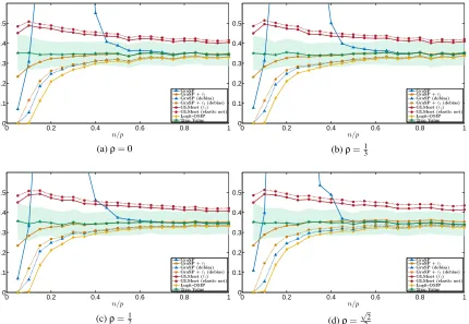
Figure 1 compares the average value of the empirical logistic loss achieved by each of the
con-sidered algorithms for a wide range of “sampling ratio”n/p. For GraSP, the curves labelled by
GraSP and GraSP +ℓ2corresponding to the cases where the algorithm is applied to unregularized
andℓ2-regularized logistic loss, respectively. Furthermore, the results of GLMnet for the LASSO
and the elastic net regularization are labelled by GLMnet (ℓ1) and GLMnet (elastic net), respectively.
The simulation result of the Logit-OMP algorithm is also included. To contrast the obtained results we also provided the average of empirical logistic loss evaluated at the true parameter and one stan-dard deviation above and below this average on the plots. Furthermore, we evaluated performance of GraSP with the debiasing procedure described in Section 3.1.
As can be seen from the figure at lower values of the sampling ratio GraSP is not accurate and does not seem to be converging. This behavior can be explained by the fact that without regular-ization at low sampling ratios the training data is linearly separable or has very few mislabelled samples. In either case, the value of the loss can vary significantly even in small neighborhoods. Therefore, the algorithm can become too sensitive to the pruning step at the end of each iteration. At larger sampling ratios, however, the loss from GraSP begins to decrease rapidly, becoming
ef-fectively identical to the loss at the true parameter for n/p>0.7. The results show that unlike
GraSP, Logit-OMP performs gracefully at lower sampling ratios. At higher sampling ratios, how-ever, GraSP appears to yield smaller bias in the loss value. Furthermore, the difference between the loss obtained by the LASSO and the loss at the true parameter never drops below a certain threshold, although the convex method exhibits a more stable behaviour at low sampling ratios.
Interestingly, GraSP becomes more stable at low sampling ratios when the logistic loss is
reg-ularized with theℓ2-norm. However, this stability comes at the cost of a bias in the loss value at
high sampling ratios that is particularly pronounced in Figure 1d. Nevertheless, for all of the tested
values of ρ, at low sampling ratios GraSP+ℓ2 and at high sampling ratios GraSP are consistently
0 0.2 0.4 0.6 0.8 1 0
0.1 0.2 0.3 0.4 0.5
n/p
GraSP GraSP +ℓ2
GraSP (debias) GraSP +ℓ2(debias) GLMnet (ℓ1) GLMnet (elastic net) Logit-OMP True Value
(a)ρ=0
0 0.2 0.4 0.6 0.8 1
0 0.1 0.2 0.3 0.4 0.5
n/p
GraSP GraSP +ℓ2
GraSP (debias) GraSP +ℓ2(debias) GLMnet (ℓ1) GLMnet (elastic net) Logit-OMP True Value
(b)ρ=1 3
0 0.2 0.4 0.6 0.8 1
0 0.1 0.2 0.3 0.4 0.5
n/p
GraSP GraSP +ℓ2
GraSP (debias) GraSP +ℓ2(debias)
GLMnet (ℓ1)
GLMnet (elastic net) Logit-OMP True Value
(c)ρ=1 2
0 0.2 0.4 0.6 0.8 1
0 0.1 0.2 0.3 0.4 0.5
n/p
GraSP GraSP +ℓ2
GraSP (debias) GraSP +ℓ2(debias)
GLMnet (ℓ1)
GLMnet (elastic net) Logit-OMP True Value
(d)ρ=√22
Figure 1: Comparison of the average (empirical) logistic loss at solutions obtained via GraSP,
GraSP withℓ2-penalty, LASSO, the elastic-net regularization, and Logit-OMP. The
re-sults of both GraSP methods with “debiasing” are also included. The average loss at the true parameter and one standard deviation interval around it are plotted as well.
appears to have a stabilizing effect at lower sampling ratios. For GraSP withℓ2regularized cost, the
debiasing particularly reduced the undesirable bias atρ=√22.
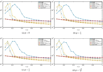
Figure 2 illustrates the performance of the same algorithms in terms of the relative error kbx−x⋆k2
kx⋆k
2
wherebxdenotes the estimate that the algorithms produce. Not surprisingly, none of the algorithms
attain an arbitrarily small relative error. Furthermore, the parameterρ does not appear to affect
the performance of the algorithms significantly. Without the ℓ2-regularization, at high sampling
ratios GraSP provides an estimate that has a comparable error versus theℓ1-regularization method.
However, for mid to high sampling ratios both GraSP and GLMnet methods are outperformed by Logit-OMP. At low to mid sampling ratios, GraSP is unstable and does not converge to an estimate close to the true parameter. Logit-OMP shows similar behavior at lower sampling ratios.
Perfor-mance of GraSP changes dramatically once we consider theℓ2-regularization and/or the debiasing
procedure. Withℓ2-regularization, GraSP achieves better relative error compared to GLMnet and
0 0.2 0.4 0.6 0.8 1 10−1
100 101 102
n/p
GraSP GraSP +ℓ2
GraSP (debias) GraSP +ℓ2(debias)
GLMnet (ℓ1) GLMnet (elastic net) Logit-OMP
(a)ρ=0
0 0.2 0.4 0.6 0.8 1
10−1 100 101 102
n/p
GraSP GraSP +ℓ2
GraSP (debias) GraSP +ℓ2(debias)
GLMnet (ℓ1) GLMnet (elastic net) Logit-OMP
(b)ρ=13
0 0.2 0.4 0.6 0.8 1
10−1 100 101 102
n/p
GraSP GraSP +ℓ2
GraSP (debias) GraSP +ℓ2(debias) GLMnet (ℓ1) GLMnet (elastic net) Logit-OMP
(c)ρ=12
0 0.2 0.4 0.6 0.8 1
10−1 100 101 102
n/p
GraSP GraSP +ℓ2
GraSP (debias) GraSP +ℓ2(debias) GLMnet (ℓ1) GLMnet (elastic net) Logit-OMP
(d)ρ=√22
Figure 2: Comparison of the average relative error (i.e., kbx−x⋆k2
kx⋆k
2 ) in logarithmic scale at solutions
obtained via GraSP, GraSP withℓ2-penalty, LASSO, the elastic-net regularization, and
Logit-OMP. The results of both GraSP methods with “debiasing” are also included.
These variants of GraSP appear to perform better than Logit-OMP for almost the entire range of
n/p.
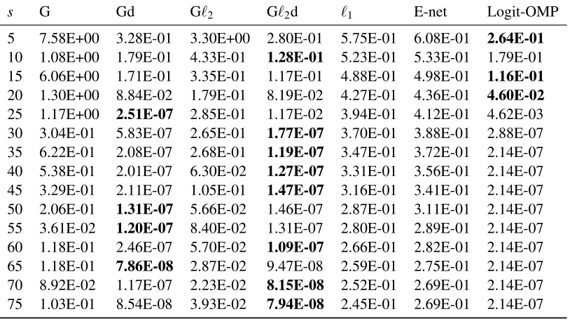
5.2 Real Data
We also conducted the same simulation on some of the data sets used in NIPS 2003 Workshop on feature extraction (Guyon et al., 2005), namely the ARCENE and DEXTER data sets. The logistic loss values at obtained estimates are reported in Tables 2 and 3. For each data set we applied the
sparse logistic regression for a range of sparsity levels. The columns indicated by “G” correspond
to different variants of GraSP. Suffixesℓ2 and “d” indicate theℓ2-regularization and the debiasing
are applied, respectively. The columns indicated byℓ1 and E-net correspond to the results of the
ℓ1-regularization and the elastic-net regularization methods that are performed using the GLMnet
package. The last column contains the result of the Logit-OMP algorithm.
s G Gd Gℓ2 Gℓ2d ℓ1 E-net Logit-OMP
5 5.89E+01 5.75E-01 2.02E+01 5.24E-01 5.59E-01 6.43E-01 2.23E-01
10 3.17E+02 5.43E-01 3.71E+01 4.53E-01 5.10E-01 5.98E-01 5.31E-07
15 3.38E+02 6.40E-07 5.94E+00 1.42E-07 4.86E-01 5.29E-01 5.31E-07
20 1.21E+02 3.44E-07 8.82E+00 3.08E-08 4.52E-01 5.19E-01 5.31E-07
25 9.87E+02 1.13E-07 4.46E+01 1.35E-08 4.18E-01 4.96E-01 5.31E-07
Table 2: ARCENE
s G Gd Gℓ2 Gℓ2d ℓ1 E-net Logit-OMP
5 7.58E+00 3.28E-01 3.30E+00 2.80E-01 5.75E-01 6.08E-01 2.64E-01
10 1.08E+00 1.79E-01 4.33E-01 1.28E-01 5.23E-01 5.33E-01 1.79E-01
15 6.06E+00 1.71E-01 3.35E-01 1.17E-01 4.88E-01 4.98E-01 1.16E-01
20 1.30E+00 8.84E-02 1.79E-01 8.19E-02 4.27E-01 4.36E-01 4.60E-02
25 1.17E+00 2.51E-07 2.85E-01 1.17E-02 3.94E-01 4.12E-01 4.62E-03
30 3.04E-01 5.83E-07 2.65E-01 1.77E-07 3.70E-01 3.88E-01 2.88E-07
35 6.22E-01 2.08E-07 2.68E-01 1.19E-07 3.47E-01 3.72E-01 2.14E-07
40 5.38E-01 2.01E-07 6.30E-02 1.27E-07 3.31E-01 3.56E-01 2.14E-07
45 3.29E-01 2.11E-07 1.05E-01 1.47E-07 3.16E-01 3.41E-01 2.14E-07
50 2.06E-01 1.31E-07 5.66E-02 1.46E-07 2.87E-01 3.11E-01 2.14E-07
55 3.61E-02 1.20E-07 8.40E-02 1.31E-07 2.80E-01 2.89E-01 2.14E-07
60 1.18E-01 2.46E-07 5.70E-02 1.09E-07 2.66E-01 2.82E-01 2.14E-07
65 1.18E-01 7.86E-08 2.87E-02 9.47E-08 2.59E-01 2.75E-01 2.14E-07
70 8.92E-02 1.17E-07 2.23E-02 8.15E-08 2.52E-01 2.69E-01 2.14E-07
75 1.03E-01 8.54E-08 3.93E-02 7.94E-08 2.45E-01 2.69E-01 2.14E-07
Table 3: DEXTER
Logit-OMP has the best performance, the smallest loss values in both data sets are attained by GraSP methods with debiasing step.
6. Discussion and Conclusion
In many applications understanding high dimensional data or systems that involve these types of data can be reduced to identification of a sparse parameter. For example, in gene selection problems researchers are interested in locating a few genes among thousands of genes that cause or contribute to a particular disease. These problems can usually be cast as sparsity-constrained optimizations. In this paper we introduce a greedy algorithm called the Gradient Support Pursuit(GraSP) as an approximate solver for a wide range of sparsity-constrained optimization problems.
sparse recovery to the case of cost functions other than the squared error. To provide a concrete
example we studied the requirements of GraSP forℓ2-regularized logistic loss. Using a similar
ap-proach one can verify SRH condition for loss functions that have Lipschitz-continuous gradient that incorporates a broad family of loss functions.
At medium- and large-scale problems computational cost of the GraSP algorithm is mostly
af-fected by the inner convex optimization step whose complexity is polynomial in s. On the other
hand, for very large-scale problems, especially with respect to the dimension of the input, p, the
running time of the GraSP algorithm will be dominated by evaluation of the function and its
gradi-ent, whose computational cost grows withp. This problem is common in algorithms that only have
deterministic steps; even ordinary coordinate-descent methods have this limitation (Nesterov, 2012). Similar to improvements gained by using randomization in coordinate-descent methods (Nesterov, 2012), introducing randomization in the GraSP algorithm could reduce its computational complex-ity at large-scale problems. This extension, however, is beyond the scope of this paper and we leave it for future work.
Appendix A. Iteration Analysis For Smooth Cost Functions
To analyze our algorithm we first establish a series of results on how the algorithm operates on its current estimate, leading to an iteration invariant property on the estimation error. Propositions 1 and 2 are used to prove Lemmas 1 and 2. These Lemmas then are used to prove Lemma 3 that provides an iteration invariant which in turn yields the main result.
Proposition 1. LetM(t)be a matrix-valued function such that for all t∈[0,1],M(t)is symmetric and its eigenvalues lie in interval[B(t),A(t)]with B(t)>0. Then for any vectorvwe have
1
Z
0 B(t)dt
kvk2≤
1
Z
0
M(t)dt v
2≤
1
Z
0 A(t)dt
kvk2.
Proof Letλmin(·)andλmax(·)denote the smallest and largest eigenvalue functions defined over the
set of symmetric positive-definite matrices, respectively. These functions are in order concave and convex. Therefore, Jensen’s inequality yields
λmin
1
Z
0
M(t)dt ≥
1
Z
0
λmin(M(t))dt≥ 1
Z
0 B(t)dt
and
λmax
1
Z
0
M(t)dt ≤
1
Z
0
λmax(M(t))dt≤ 1
Z
0
A(t)dt,
Proposition 2. LetM(t)be a matrix-valued function such that for all t∈[0,1]M(t)is symmetric and its eigenvalues lie in interval[B(t),A(t)]with B(t)>0. IfΓis a subset of row/column indices ofM(·)then for any vectorvwe have
1
Z
0
PTΓM(t)PΓcdt v
2
≤ 1
Z
0
A(t)−B(t)
2 dtkvk2.
Proof SinceM(t)is symmetric, it is also diagonalizable. Thus, for any vectorvwe may write
B(t)kvk22≤vTM(t)v≤A(t)kvk22,
and thereby
−A(t)−2B(t) ≤
vTM(t)−A(t)+2B(t)Iv
kvk2 ≤
A(t)−B(t)
2 .
SinceM(t)−A(t)+2B(t)Iis also diagonalizable, it follows from the above inequality that
M(t)−
A(t) +B(t)
2 I
≤
A(t)−B(t)
2 .
LetMe(t) =PΓTM(t)PΓc. SinceMe(t)is a submatrix ofM(t)−A(t)+B(t)
2 Iwe should have
eM(t)≤
M(t)−
A(t) +B(t)
2 I
≤
A(t)−B(t)
2 . (11)
Finally, it follows from the convexity of the operator norm, Jensen’s inequality, and (11) that
1
Z
0 e
M(t)dt ≤
1
Z
0
eM(t)dt≤ 1
Z
0
A(t)−B(t)
2 dt.
To simplify notation we introduce functions
αk(p,q) =
1
Z
0
Ak(tq+ (1−t)p)dt
βk(p,q) =
1
Z
0
Bk(tq+ (1−t)p)dt
γk(p,q) =αk(p,q)−βk(p,q),
Lemma 1. Let
R
denote the setsupp(bx−x⋆). The current estimatebxthen satisfiesk(bx−x⋆)|Zck2≤
γ4s(bx,x⋆)+γ2s(bx,x⋆)
2β2s(bx,x⋆) kb
x−x⋆k2+
∇f(x⋆)|
R\Z
2+
∇f(x⋆)|
Z\R
2
β2s(bx,x⋆)
.
Proof Since
Z
=supp(z2s)and|R
| ≤2swe havez|R
2≤ kz|Zk2and thereby
z|R\Z
2≤ z|Z\R
2. (12)
Furthermore, becausez=∇f(bx)we can write
z|R\Z
2≥
∇f(bx)|R\Z−∇f(x⋆)|R\Z
2−
∇f(x⋆)|R\Z
2 = 1 Z 0
PTR\ZHf(txb+ (1−t)x⋆)dt
(bx−x⋆)
2−
∇f(x⋆)|R\Z
2 ≥ 1 Z 0
PTR\ZHf(tbx+ (1−t)x⋆)PR\Zdt
(bx−x⋆)|R\Z
2
−∇f(x⋆)|R\Z
2 − 1 Z 0
PTR\ZHf(tbx+ (1−t)x⋆)PZ∩Rdt
(bx−x⋆)|Z∩R
2,
where we split the active coordinates (i.e.,
R
) into the setsR
\Z
andZ
∩R
to apply the triangleinequality and obtain the last expression. Applying Propositions 1 and 2 yields
z|R\Z
2≥β2s(bx,x
⋆)(bx−x⋆)|
R\Z
2−
γ2s(bx,x⋆)
2
(bx−x⋆)|Z∩R
2−
∇f(x⋆)|R\Z
2 ≥β2s(bx,x⋆)
(bx−x⋆)|R\Z
2−
γ2s(bx,x⋆)
2 kbx−x
⋆k 2−
∇f(x⋆)|R\Z
2. (13)
Similarly, we have
z|Z\R
2≤
∇f(bx)|Z\R −∇f(x⋆)|Z\R
2+
∇f(x⋆)|Z\R
2 = 1 Z 0
PTZ\RHf(tbx+ (1−t)x⋆)PRdt
(bx−x⋆)|R
2+
∇f(x⋆)|Z\R
2 ≤γ4s(bx,x
⋆)
2
(bx−x⋆)|R
2+
∇f(x⋆)|Z\R
2
=γ4s(bx,x
⋆)
2 kbx−x
⋆k 2+
∇f(x⋆)|Z\R
2. (14)
Combining (12), (13), and (14) we obtain
γ4s(bx,x⋆)
2 kbx−x
⋆k 2+
∇f(x⋆)|Z\R
2≥ z|Z\R
2 ≥z|R\Z
2
≥β2s(bx,x⋆)
(bx−x⋆)|R\Z
2−
γ2s(bx,x⋆)
2 kbx−x
⋆ k2 −∇f(x⋆)|R\Z
Since
R
=supp(bx−x⋆), we have(bx−x⋆)|R\Z
2=k(bx−x ⋆)|
Zck2. Hence, k(bx−x⋆)|Zck2≤γ4s(bx,x
⋆)+γ
2s(bx,x⋆)
2β2s(bx,x⋆) kb
x−x⋆k2+
∇f(x⋆)|R\Z
2+∇f(x⋆)|Z\R
β2s(bx,x⋆)
.
Lemma 2. The vectorbgiven by
b=arg minf(x) s.t.x|Tc=0 (15)
satisfies
kx⋆|T−bk2≤k∇f(x
⋆)|
Tk2
β4s(b,x⋆)
+ γ4s(b,x
⋆)
2β4s(b,x⋆)k
x⋆|Tck2.
Proof We have
∇f(x⋆)−∇f(b) =
1
Z
0
Hf(tx⋆+(1−t)b)dt(x⋆−b).
Furthermore, sincebis the solution to (15) we must have∇f(b)|T =0. Therefore,
∇f(x⋆)|T =
1
Z
0
PTTHf(tx⋆+ (1−t)b)dt
(x⋆−b)
=
1
Z
0
PTTHf(tx⋆+(1−t)b)PTdt
(x⋆−b)|T
+
1
Z
0
PTTHf(tx⋆+(1−t)b)PTcdt
(x⋆−b)|Tc. (16)
Since f hasµ4s-SRH and |
T
∪supp(tx⋆+ (1−t)b)| ≤4s for all t∈[0,1], functions A4s(·) andB4s(·), defined using (5) and (6), exist such that we have
B4s(tx⋆+ (1−t)b)≤λmin PTTHf(tx⋆+(1−t)b)PT
and
A4s(tx⋆+ (1−t)b)≥λmax PTTHf(tx⋆+(1−t)b)PT.
Thus, from Proposition 1 we obtain
β4s(b,x⋆)≤λmin
1
Z
0
PTTHf(tx⋆+ (1−t)b)PTdt
and
α4s(b,x⋆)≥λmax
1
Z
0
PTTHf(tx⋆+ (1−t)b)PTdt
.
This result implies that the matrix R01PT
THf(tx⋆+ (1−t)b)PTdt, henceforth denoted by W, is
invertible and
1
α4s(b,x⋆) ≤
λmin W−1
≤λmax W−1
≤β 1 4s(b,x⋆)
, (17)
where we used the fact thatλmax(M)λmin M−1
=1 for any positive-definite matrixM, particularly
forWandW−1. Therefore, by multiplying both sides of (16) byW−1obtain
W−1∇f(x⋆)|T = (x⋆−b)|T +W−1
1
Z
0
PTTHf(tx⋆+(1−t)b)PTcdt x⋆|Tc,
where we also used the fact that(x⋆−b)|
Tc=x⋆|Tc. With
S
⋆=supp(x⋆), using triangle inequality,(17), and Proposition 2 then we obtain
kx⋆|T−bk2=k(x⋆−b)|Tk2
≤
W
−1
1
Z
0
PTTHf(tx⋆+(1−t)b)PTc∩S⋆dt
x⋆|Tc∩S⋆
2+
W−1∇f(x⋆)|T
2
≤k∇f(x ⋆)|
Tk2
β4s(b,x⋆)
+ γ4s(b,x
⋆)
2β4s(b,x⋆)k
x⋆|Tck2,
as desired.
Lemma 3(Iteration Invariant). The estimation error in the current iteration,kbx−x⋆k2, and that in the next iteration,kbs−x⋆k2, are related by the inequality:
kbs−x⋆k2≤
γ4s(bx,x⋆) +γ2s(bx,x⋆)
2β2s(bx,x⋆)
1+γ4s(b,x
⋆)
β4s(b,x⋆)
kbx−x⋆k2
+
1+γ4s(b,x
⋆)
β4s(b,x⋆)
∇f(x⋆)|R\Z
2+
∇f(x⋆)|Z\R
2
β2s(bx,x⋆)
+2k∇f(x
⋆)|
Tk2 β4s(b,x⋆)
.
Proof Because
Z
⊆T
we must haveT
c⊆Z
c. Therefore, we can writekx⋆|Tck2=k(bx−x⋆)|Tck2≤
k(bx−x⋆)|Zck2. Then using Lemma 1 we obtain
kx⋆|Tck2≤
γ4s(bx,x⋆)+γ2s(bx,x⋆)
2β2s(bx,x⋆) kb
x−x⋆k2+
∇f(x⋆)|R\Z
2+
∇f(x⋆)|Z\R
2
β2s(bx,x⋆)
. (18)
Furthermore,
kbs−x⋆k2≤ kbs−x⋆|Tk2+kx⋆|Tck2
where the last inequality holds becausekx⋆|Tk0≤sandbsis the bests-term approximation ofb.
Therefore, using Lemma 2,
kbs−x⋆k2≤
2
β4s(b,x⋆)k
∇f(x⋆)|Tk2+
1+γ4s(b,x
⋆)
β4s(b,x⋆)
kx⋆|Tck2. (20)
Combining (18) and (20) we obtain
kbs−x⋆k2≤
γ4s(bx,x⋆) +γ2s(bx,x⋆)
2β2s(bx,x⋆)
1+γ4s(b,x
⋆)
β4s(b,x⋆)
kbx−x⋆k2
+
1+γ4s(b,x
⋆)
β4s(b,x⋆)
∇f(x⋆)|
R\Z
2+
∇f(x⋆)|
Z\R
2
β2s(bx,x⋆)
+2k∇f(x
⋆)|
Tk2
β4s(b,x⋆)
.
Using the results above, we can now prove Theorem 1.
Proof of Theorem1. Using definition 1 it is easy to verify that fork≤k′ and any vectoruwe
haveAk(u)≤Ak′(u) andBk(u)≥Bk′(u). Consequently, fork≤k′and any pair of vectorspand
qwe haveαk(p,q)≤αk′(p,q),βk(p,q)≥βk′(p,q), andµk≤µk′. Furthermore, for any function
that satisfiesµk−SRH we can write
αk(p,q) βk(p,q)
=
R1
0Ak(tq+ (1−t)p)dt
R1
0Bk(tq+ (1−t)p)dt
≤
R1
0µkBk(tq+ (1−t)p)dt
R1
0 Bk(tq+ (1−t)p)dt
=µk,
and thereby γk(p,q)
βk(p,q)≤µk−1. Therefore, applying Lemma 3 to the estimate in thei-th iterate of the
algorithm shows that
bx(i)−x⋆
2≤(µ4s−1)µ4s
bx(i−1)−x⋆
2+
2k∇f(x⋆)|
Tk2
β4s(b,x⋆)
+µ4s
∇f(x⋆)|R\Z
2+∇f(x⋆)|Z\R
2
β2s bx(i−1),x⋆
≤ µ24s−µ4sbx(i−1)−x⋆
2+2
εk∇f(x
⋆)
|Ik2+2µ4s ε k∇f(x
⋆) |Ik2.
Applying the assumptionµ4s≤1+
√
3
2 then yields
bx(i)−x⋆
2≤12bx(i−1)−x⋆
2+3+
√
3
ε k∇f(x
⋆)|
Ik2.
The theorem follows using this inequality recursively.
Appendix B. Iteration Analysis For Non-Smooth Cost Functions
In this part we provide analysis of GraSP for non-smooth functions. Definition 3 basically states
that for anyk-sparse vectorx∈Rn,αk(x)andβk(x)are in order the smallest and largest values for
which