Regularized Bundle Methods for Convex and Non-Convex Risks
Trinh-Minh-Tri Do∗ [email protected]
Idiap Research Institute Rue Marconi 19
1920 Martigny, Switzerland
Thierry Arti`eres [email protected]
LIP6 - Universit´e Pierre et Marie Curie 104 avenue du pr´esident Kennedy 75016 Paris, France
Editor:Tony Jebara
Abstract
Machine learning is most often cast as an optimization problem. Ideally, one expects a convex ob-jective function to rely on efficient convex optimizers with nice guarantees such as no local optima. Yet, non-convexity is very frequent in practice and it may sometimes be inappropriate to look for convexity at any price. Alternatively one can decide not to limita priorithe modeling expressivity to models whose learning may be solved by convex optimization and rely on non-convex optimiza-tion algorithms. The main motivaoptimiza-tion of this work is to provide efficient and scalable algorithms for non-convex optimization. We focus on regularized unconstrained optimization problems which cover a large number of modern machine learning problems such as logistic regression, conditional random fields, large margin estimation, etc. We propose a novel algorithm for minimizing a regu-larized objective that is able to handle convex and non-convex, smooth and non-smooth risks. The algorithm is based on the cutting plane technique and on the idea of exploiting the regularization term in the objective function. It may be thought as a limited memory extension of convex regu-larized bundle methods for dealing with convex and non convex risks. In case the risk is convex the algorithm is proved to converge to a stationary solution with accuracyεwith a rateO(1/λε) whereλis the regularization parameter of the objective function under the assumption of a Lips-chitz empirical risk. In case the risk is not convex getting such a proof is more difficult and requires a stronger and more disputable assumption. Yet we provide experimental results on artificial test problems, and on five standard and difficult machine learning problems that are cast as convex and non-convex optimization problems that show how our algorithm compares well in practice with state of the art optimization algorithms.
Keywords: optimization, non-convex, non-smooth, cutting plane, bundle method, regularized risk
1. Introduction
Machine learning is most often cast as an optimization problem where one looks for the best model among a parameterized family of models. The best model is defined as the one with the set of pa-rameters that minimizes an objective function (i.e. criterion). For some years now machine learning community aimed at designing new models in such a way that the resulting objective function is convex. Doing so brings the fundamental advantage that one can rely on efficient convex
tion algorithms, with nice guarantees such as no local optima and easier theoretical analysis (e.g. for the convergence rate). For instance logistic regression, support vector machine, maximum mar-gin Markov network, and conditional random fields have found widespread use in basic machine learning applications.
However, such a “simple convex modeling” may actually be outperformed by non-convex mod-eling in some important applications. For example on MNIST database, convex Gaussian-SVM reaches 1.4% error rate vs. 0.53% for non-convex convolutional nets (Jarrett et al., 2009).1 Also non-convexity is much more frequent than convexity “in real life”. A number of problems that machine learning researchers face today may not be easily cast as convex optimization problems without limitinga priorithe expressivity of the models used and the potential of the models to learn (LeCun et al., 1998; Collobert et al., 2006; Bengio and Lecun, 2007). First, many real-world prob-lems need complicated models whose learning requires solving non-convex optimization probprob-lems. For instance, models with non-convex discriminant function such as neural networks and hidden Markov models (HMMs) have become classical and reference models for many difficult tasks in vi-sion and speech. Second, non-convexity of objective function naturally arises in learning paradigms such as unsupervised and semi-supervised learning as well as in transductive SVM, etc (Chapelle et al., 2006; Joachims, 1999).
Two strategies have been investigated to handle non-convexity in machine learning approaches. Few works attempted to use convex relaxation technique in order to transform an original non-convex problem into a non-convex one, this is a kind of “non-convexity at any price” strategy. Convex relaxation mechanics strongly depend on the application, there is no principled method for turning a non-convex problem to a convex one. It has been used in maximum margin clustering (Xu et al., 2004), transductive SVM (Xu et al., 2008), discriminative unsupervised structured predictors (Xu et al., 2006), large margin CDHMM (Sha and Saul, 2007). However, the robustness of this ap-proach for complex problems is questionable since the use of strong assumptions may lead to poor approximation quality, thus provide poor performance in practice.
Since convex modeling does not cover all real-world problems and convex relaxation techniques are not always easy and robust, few researchers proposed to give up convexity and to focus on non-convex optimization techniques, for instance concave-convex procedure (CCCP) (Yuille and Rangarajan, 2003) and difference of convex (DC) programming (Horst and Thoai, 1999). These non-convex optimization techniques have been successfully applied for some tasks such as ramp loss SVM, non-convex TSVM (Collobert et al., 2006), kernel selection (Argyriou et al., 2006) or non-convex maximum margin clustering (Zhao et al., 2008). Note that these techniques cover only a limited class of problems and require an ad-hoc design for every machine learning problem. For instance, the CCCP can theoretically be applied to any continuous objective function since any such function can be decomposed into the difference of two convex functions, yet reformulating the original function to a concave-convex form may call for mathematical efforts. Furthermore not all decomposition are interesting.
We are concerned here with the development of generic optimization techniques able to deal with the general unconstrained optimization problem
minw f(w)
with f(w) =λ2kwk2+R(w) (1)
wherew∈RD are the model parameters andR(w)(the main objective) is a data-fitting
measure-ment to be minimized which we consider to be not necessarily smooth everywhere nor convex. This unconstrained formulation covers many mentioned machine learning problems such as SVM, CRF, M3N, transductive SVM, ramp loss SVM, neural network (Do and Arti`eres, 2010), Gaussian HMM (Do and Arti`eres, 2009). Note that the formulation in Equation 1 does not apply easily to kernel methods which are based on an implicit data transformation (e.g. RBF kernel) and are preferably solved in the dual space. However, there are several methods that can enrich the model flexibility without considering an implicit data transformation. As an example, for low dimensional or sparse data, one could have an explicit and efficient transformation for polynomial kernel. Furthermore, instead of using a predefined implicit transformation one could also learn the explicit data transfor-mation directly such as latent feature discovery based on Boltzmann machine (Hinton et al., 2006). At the end, while not covering kernel tricks, our general optimization problem can be used for learning many powerful non-linear models.
As the problem in Equation 1 is at the heart of many machine learning application, it is important to have an efficient non-convex optimization method for this class of minimization problem. Among candidate families of optimization algorithms, cutting plane methods and bundle based methods are very appealing for optimization problems such as the one in Equation 1 since, as opposed to many gradient descent based methods, it can naturally deal with its non-smooth everywhere fea-ture (Kiwiel, 1985; Gaudioso and Monaco, 1992; Makela, 2002; Makela and Neittaanmaki, 1992; Schramm and Zowe, 1992). However the convergence of bundle methods for non-convex optimiza-tion is rather slow in practice. And theoretical results on convergence rate are indeed missing for non-convex objective functions. This explains in our opinion why the use of general non-convex bundle methods is still limited in machine learning. Another reason is the lack of easy-to-use im-plementation of non-convex bundle methods.
The recent success of convex regularized bundle methods (CRBMs) in machine learning (Smola et al., 2008; Weimer et al.; Joachims et al., 2009) motivated us to investigate extensions of bundle methods for proposing efficient algorithms able to deal with machine learning non-convex optimiza-tion problems, which is the core idea of this work. To design such an algorithm, we investigated new optimization algorithms that combines ideas from non-convex bundle methods (NBM) (Ki-wiel, 1985) and from CRBMs (Smola et al., 2008). Our algorithm relies on two main contributions, a limited memory variant of bundle methods and the extension of CRBM to non-convex risks.
The limited memory variant may be used in CRBM as well as in our non-convex extension of CRBM. It allows limiting the algorithmic complexity of a single iteration in bundle methods while it is usually increasing (at least quadratically) with the number of iteration, which makes bundle methods not practical for difficult and large scale problems requiring thousands of iterations. We show that our limited memory variant, when included to CRBM, inherits its fast convergence rate inO(1/λε)iteration to reach a gap belowε.
Our extension of CRBM to non-convex risks includes the limited memory variant and is de-signed to make bundle methods scalable for real life non-convex learning problems.2 This is achieved by making the algorithm focus on the current best solution and by using a specific lo-cality measure for regularized risks. Such a strategy allows fast convergence in practice on difficult and large scale machine learning problems that we investigated. Unfortunately this comes with only weak proof of convergence towards a stationary solution, relying on a moot assumption. In our
opinion it is a kind of trade-off, a price to pay to achieve algorithmic efficiency in practice. As a consequence though we provide main theoretical results we do not include our convergence proofs here since these are weak, but these are available in an internal report (Do and Artieres, 2012).
First, in Section 2 we provide background on the cutting plane technique and on bundle meth-ods, and we describe two main existing extensions, the convex regularized bundle method (CRBM) and the non-convex bundle method (NBM). Then, we present in Section 3 our two contributions yielding our algorithm, NRBM, which is a regularized bundle method for non-convex optimization. We propose few variants of our method in Section 3.3 and we discuss in Section 4 the convergence behavior of our method both for convex risks and for non-convex risks. Finally we provide in Section 5 a number of experimental results. We investigate first artificial test problems that show that our algorithm compares well to standard non-convex bundle methods while converging much faster, suggesting our algorithm may make large scale problems practical. Second we compare our algorithms to dedicated state of the arts optimization algorithms for a number of machine learning problems, including standard problems such as learning of transductive support vector machines learning, learning of maximum margin Markov networks, learning conditional random fields, as well as less standard but difficult optimization problems related to discriminative training of com-plex graphical models for handwriting and speech recognition.
2. Background on Cutting Plane and Bundle Methods
We provide now some background on the cutting plane principle and on optimization methods that have been built on this idea for convex and non-convex objective functions.
2.1 Cutting Plane Principle
Surely the most powerful method for non-smooth optimization is based onpolyhedral approxima-tions, whose basic element is thecutting plane (CP). For a given function f(w), a cutting plane
cw′(w)is a first-order Taylor approximation computed at a particular pointw′: f(w)≈cw′(w) = f(w′) +haw′,w−w′i
where aw′ ∈∂f(w′) is a subgradient of f atw′. For convex function, the subdifferential ∂f(w′)
is the set of vectorsa that satisfies: f(w)≥ f(w′) +haw′,w−w′i. The concept of subdifferential
is also generalized for non-convex functions, which is defined as the set of vectorsathat satisfies:
f◦(w′;h)≥ ha,hi ∀h, where f◦(w′,h)denotes the generalized directional derivative of f atw′ in the directionh.
Go back to the definition of the cutting plane approximation based on Taylor approximation, it may be rewritten as:
cw′(w) =haw′,wi+bw′ with aw′ ∈∂f(w′)
bw′ = f(w′)− haw′,w′i.
(2)
A cutting planecw′is an approximation of fwhich is accurate forwlying in the vicinity ofw′where
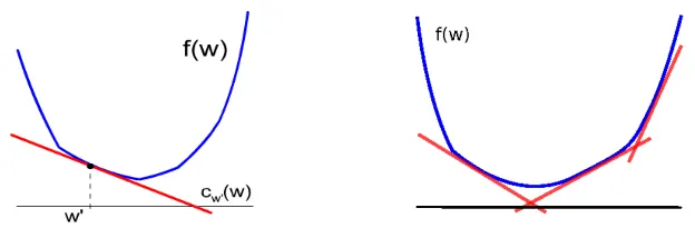
Figure 1: Basic approximation of a function f by a (underestimator) cutting plane at a point w′ (left), and a more accurate approximation by taking the maximum over many cutting planes of f (right).
2.2 Cutting Plane Method for a Convex Objective
Thecutting plane methodhas been proposed for the minimization of convex functions. In the case of a convex objective, any cutting plane of the objective f is an underestimator of f. The idea of the cutting plane method is that one can build an accurate approximation function (namedgt hereafter)
of f, which is also an underestimator of f, as the maximum over many cutting plane approximation built at different points{w1, ...,wt}as follows:
f(w)≈gt(w) =max
j=1..thawj,wi+bwj. (3)
Of coursegt(w)is an underestimator off(w). It is called the approximation function of fat iteration
t.
The cutting plane method aims at iteratively building an increasingly accurate piecewise linear underestimator of the objective function by successively adding new cutting planes to the approx-imationg of f. If the approximation is good enough, one may hope that the minimum of f and of its approximationg will be very close or even equal. Every iteration, one adds a new cutting plane underestimator built at current solution, yielding a new piece-wise linear underestimator of
f as in Equation 3. The minimization of this underestimator approximation is usually called the approximated problem (it is a linear program) and gives a new current solution, etc.
Note that the approximation function may not have a minimum, then artificial bounds may be placed on the points of w, so that the minimization will be carried out over a compact set and consequently a exists.
The cutting plane method is described in Algorithm 1, it is proved to converge in a finite number of iterations to anε-solution (Bertsekas et al., 2003).
2.3 Bundle Methods for a Convex Risk
Algorithm 1Cutting Plane Method (for convex objective function)
1: Input: w1, f,ε
2: Output: w∗
3: for t=1 to∞do
4: Computeawt andbwt according to Equation 2
5: Minimizegt(w)(defined as in Equation 3) to getwt+1←argminwgt(w)
6: gap= [minj=1..t f(wj)]−gt(wt+1)
7: ifgap<εthen return wt
8: end for
Algorithm 2Convex Regularized Bundle Method (CRBM)
1: Input: w1,R,ε
2: Output: w∗
3: for t=1 to∞do
4: Computeawt andbwt ofRatwt 5: w∗t =argminw∈{w1,...wt}f(w)
6: w˜t←argminwgt(w)wheregt(w)is defined as in Equation 6
7: gapt= f(w∗t)−gt(w˜t)
8: wt+1=w˜t
9: ifgapt<εthen return wt∗
10: end for
term. The approximation function becomes:
f(w)≈gt(w) = (w−wt)⊤Ht(w−wt) +max
j=1..thawj,wi+bwj (4)
whereHt is a positive definite symmetric matrix. The regularization term forces the new solution not
to be too far from the current solution. In addition it makes the approximation function have a unique minimum (as long as the Hessian matrix of the regularization term is positive-definite as in our example) without adding artificial constraints. While the approximation function in Equation 4 can be used to generate new points, the standard bundle method also includes a line-search procedure which returns either a serious step (the objective at current solution has significantly decreased) or a null step (the decrease of f is too low and the approximation function should be improved).
Convex regularized bundle method. The convex regularized bundle method (CRBM) (Smola et al., 2008) is an instance of CBM algorithms for dealing with regularized (and convex) risks as in Equa-tion 1. It relies on cutting planes that are built on the riskR(w)only and does not use a line search procedure. Such a linear approximation of the risk R(w)yields a quadratic approximation of the objective f(w):
f(w)≈λ
2kwk 2+ha
w′,wi+bw′. (5)
These two approximation functions on R(w) and on f(w) are illustrated in Figure 2. Note that this quadratic approximation of f(w) is more accurate than a cutting plane approximation on
Figure 2: Cutting plane approximations in CRBM : A linear underestimator of R(w) (a), and a quadratic underestimator of f(w) =λ2kwk2+R(w)derived from this linear underestima-tor (b) (Cf. Equation 5)
CRBM is very similar to the cutting plane technique described before, where every iteration a new cutting plane approximation is built (at the current solution) and added to the current approxi-mation function. The approxiapproxi-mation of f(w)at iterationtis then:
f(w)≈gt(w) = λ
2kwk
2+max
j=1..thawj,wi+bwj (6)
and the approximation problem is
˜
wt =argmin
w
gt(w) =argmin
w
λ
2kwk
2+max
j=1..thawj,wi+bwj (7)
wherehawj,wi+bwj is the approximation cutting plane of Rbuilt atwj, the solution at iteration j. Importantly, if R(w) is convex then any cutting planehawj,wi+bwj is an underestimator of R(w), and its maximum, maxj=1..thawj,wi+bwj, is also an underestimator approximation of R.
Hence,gt(w)are monotonically increasing quadratic underestimators of f(w)which converge
to-wards f(w)as cutting planes are added.
Minimizing the approximation problem in CRBM.The approximation problem (Equation 7) at iter-ationtis an SVM-like optimization problem:
˜
wt = argminwminξ λ2kwk2+ξ
s.t. haj,wi+bj≤ξ j=1..t
with cj(w) =haj,wi+bj. We can get its dual form easily through Lagrangian mechanics. The
Lagrangian of the above optimization problem is:
L(w,ξ,α) =λ 2kwk
2+ξ+
∑
j=1..t
αj(haj,wi+bj−ξ)
where α= (α1, ...,αt) are Lagrange multipliers. The solution is given by a saddle point of the Lagrangian, that must be minimized wrt. primal variables (w,ξ) and maximized wrt. Lagrange multipliers. At a saddle point, the derivative of the Lagrangian wrt. (w,ξ) must satisfy:
∂L
∂ξ=0 ⇐⇒ ∑j=1..tαj=1,
∂L
By substituting these results back into the Lagrangian, primal variableswandξdisappear and we get the dual problem:
αt = argmax
α∈Rt − 1
2λkαAtk2+αBt s.t αj≥0∀j=1..t
∑j=1..tαj=1
(8)
whereAt = [a1;...;at]is a matrix (withajbeing row vectors),Bt= [b1;...;bt]is the vector of scalars
andαstands for the (row) vector of Lagrange multipliers (of lengthtat iterationt). Letαt be the solution of the above dual problem at iterationt, the solution of the primal problem is given by:
˜
wt =−αλtAt,
gt(w˜t) =−21λkαtAtk2+αtBt.
Convergence rate of CRBM. The convergence of CRBM is proved based on the fact that the gap between the best observed value f(w∗t) and the minimum of the approximation function gt(w˜t)
decreases every iteration. Sincegt(w)is an underestimator of f(w), the gap is greater than or equal
to the difference between the best observed value f(w∗t)and the minimum of f(w). Therefore, if
gapt ≤ε then w∗t is anε-solution of f(w). By characterizing the decrease of the gap after each
iteration, the authors of CRBM proved that the method requireO(1/λε)iterations to reach a gap belowε(Smola et al., 2008).
2.4 Non-Convex Bundle Methods (NBM)
Bundle methods have also been extended to deal with non-convex functions and have become a standard for minimizing non-smooth and non-convex function.
2.4.1 PRINCIPLE
There are many variants of non-convex bundle algorithm (NBM), with many parameters to tune. We present here a simple description of the method to better stress its main features. Basically NBM works similarly as standard bundle methods by building iteratively an approximation function via the cutting plane technique. However since the objective is no more convex, such an approximation function is not an underestimator of the objective anymore which makes things harder and requires a more complicated algorithm.
Every iteration the algorithm updates a number of quantities, whose set is usually called thestate
of the algorithm, based on the state in previous iteration. The state of the algorithm at iterationt, namedBt, is a set of points, subgradients and locality measures to the current solution. At iteration
t, the algorithm performs the following steps:
• Determine the search direction.This is done through minimizing the approximated problem
defined byBt. The approximation problem is an instance of quadratic programming similar
to the one in Equation 4, except that the raw cutting planes are adjusted to make sure that the approximation is a local underestimator of the objective function. The minimization of the approximation problem yields a new point ˜wt.
• Perform a line search. The algorithm performs a special line search from the best current
solutionw∗t to the minimum of the approximation problem ˜wt.3 The line search outputs a
new solutionwt+1. Two cases may arise. In a first case, this new solution does not lead to a significant improvement (i.e. decrease) in the objective function, we say the current iteration is a null step. In such a case, the best solution does not change (i.e.w∗t+1≡w∗t). Alternatively the new solution may bring a significant improvement in the objective (iteration is called a serious step). Then one defines the new best solution aswt∗+1≡wt+1. Note that in both cases, the approximation function is improved by adding a new cutting plane at wt+1. We do not present in details the line search procedure since it is both rather complicated and standard. Interested readers may find detailed description in the literature, e.g., (Luksan and Vlcek, 2000).
• Update the bundle and build a new approximation function. The set of cutting planes is
expanded with the new cutting plane built atwt+1. Due to the non-convex feature of the ob-jective function, the definition of approximation is not trivial, involving additional concepts such as locality measure, the strategy of NBM to deal with non-convexity will be detailed in the next subsection. Importantly, note that one gets more cutting planes in the bundle as the algorithm iterates, and such a ever increasing number of cutting planes may represent a poten-tial problem wrt. computational and memory cost if many iterations are required. Usually to overcome such a problem, one uses an aggregated cutting plane in order to accumulate infor-mation of all cutting planes in previous iterations (Kiwiel, 1985). It allows discarding older cutting planes and helps limiting the algorithmic complexity. For instance, one may keep a fixed number of cutting planes in the bundleBt by removing the oldest cutting plane. Then,
the aggregated cutting plane allows preserving part of the information brought by removed cutting planes.
2.4.2 HANDLINGNON-CONVEXOBJECTIVEFUNCTION
Bundle methods must be adapted to work for non-convex optimization since the core idea of using a first order Taylor approximation as an underestimator of the objective function does not hold anymore. Then, the standard approximation function, which is defined as the maximum over a set of cutting plane approximations, is not an underestimator of the non-convex objective function anymore. In addition although one may reasonably assume that a cutting plane built at a pointw′ is an accurate approximation of f in a small region aroundw′, such an approximation may become very poor forwfar fromw′. At the end, the maximum over cutting plane “approximations” may be a very poor approximation of the objective.
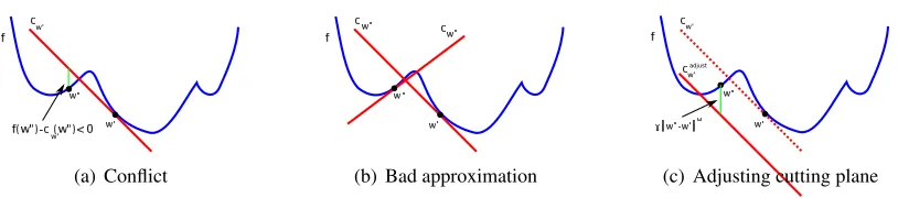
An example of poor approximation is shown in Figure 3(a). The linearization error (f(w)− cw′(w))of a cutting planecw′ at a pointw′′may be negative, meaning that the function is
overes-timated at that point. In the following we will say in such a case that there is aconflictbetween cutting planecw′ andw′′. As can be seen, overestimation of a cutting plane at a local minimum will
probably “remove” this minimum from the set of reachable solutions. Figure 3(b) shows that all three visible local minimums are “removed” by overestimation of the two cutting planes built atw′ andw′′.
Non-convex bundle method strategy. In non-convex bundle methods (Kiwiel, 1985; Gaudioso and Monaco, 1992; Makela, 2002; Makela and Neittaanmaki, 1992; Schramm and Zowe, 1992) the solution to overcome conflicts between a cutting planecw′ and a pointw′′ is to lower the cutting
planecw′ by changing its offset while preserving the normal vectoraw′ (see Figure 3(c)). This leads
to an adjusted cutting plane:
✁
✁
(a) Conflict (b) Bad approximation
✁
✁ ✂✄ ☎✆✝ ✞
(c) Adjusting cutting plane
Figure 3: Cutting planes and linearization errors.
The offsetbw′ is changed inbad just
w′ so that that the linearization error ofcad justw′ atw′′is greater than
or equal to both, the absolute value of the linearization error betweencw′ and fatw′′, and alocality measurebetweenw′andw′′:
f(w′′)−cad justw′ (w′′) ≥ |f(w′′)−cw′(w′′)|, (9)
f(w′′)−cad justw′ (w′′) ≥γkw′′−w′kω (10)
whereγ≥0,ω≥1 arelocality measure parameters. The condition (9) ensures that if the lineariza-tion error, f(w′′)−cw′(w′′), is negative then the cutting plane has to be lowered at least twice the
amount that is required to have linearization error zero. In other words, in the case of negative linearization error atw′′, the cutting plane is adjusted so that the new linearization error is posi-tive, with at least the same magnitude as the “old” negative linearization error. The condition (10) defines another underestimator on the linearization error (of the adjusted cutting plane) which is based on the distance between two pointsw′ andw′′. The further the two points are the greater the linearization error should be. The two conditions lead to the following offset change definition:
bad justw′ = f(w′′)− haw′,w′′i −max|f(w′′)−cw′(w′′)|,γkw′′−w′kω.
This is the greatest offset (closest tobw′) that satisfies the two above conditions. Besides, one can
easily check that ifcw′already satisfies both conditions (9) and (10) thenbad justw′ =bw′ andcad justw′ (w)
andcw′(w)coincide.
2.5 Conclusion
CRBM are a fast adaptation of bundle methods to convex and regularized risks. Every iteration a new cutting plane is added to the bundle so that the size of the bundle at iterationtist. This makes tackling complex tasks, eventually requiring many iterations, difficult since the cost of solving the minimization of the approximated function is quadratic in the size of the bundle. To make CRBM more scalable we will provide a limited memory variant where the size of the bundle is limited to a given size (theoretically three CP are sufficient) whatever the iteration.
3. Non-Convex Regularized Bundle Method (NRBM)
The success of convex regularized bundle methods with improved convergence rate over bundle methods, both in theory and practice, motivated us to investigate their extension to non-convex optimization, leading to bundle methods for regularized non-convex risks (NRBM). To design such an algorithm, we propose two main contributions, the extension of CRBM to non-convex risks and a limited memory variant of bundle methods that allows limiting the algorithmic cost of a single iteration.
The extension of CRBM for non-convex function is not straightforward since, as we already ob-served when presenting NBM, the cutting plane approximation does not yield an underestimator of the objective function. Our proposal is to exploit some techniques of NBM for handling non-convex function while considering a special design of the algorithm in order to keep the fast convergence rate of CRBM. On one hand, we use standard techniques such as the introduction of locality mea-sure and the adjustment of cutting planes in order to build local underestimator of the function at a given point. On the other hand, we propose novel techniques such as a particular definition of the locality measure for regularized risk and the introduction of constraints on CPs adjustment when dealing with conflicts, which guarantee a minimal improvement on the approximation gap within an iteration. At the end, we come up with a non-convex variant which inherits, in practice, the convergence rate of CRBM. Note however that we may only provide weak theoretical results on the convergence to a local minimum for the non-convex case. Convergence analysis is discussed in Section 4.
The ability of our method, NRBM, to deal with non-convex risk allows tackling a wide range of application and especially a number of everyday machine learning problems. Yet the algorithmic cost of a single iteration grows with the number of the iteration. Actually, the dual program of the approximation problem minimization in Equation 8 has a memory cost ofO(tD+t2)for storing all the cutting planes and the dot product matrix between cutting planes’ normal vectors (i.e. hai,aji),
wheretis the number of cutting planes (it is equal to the iteration number in CRBM) and D is the dimensionality of w. In addition, the computational cost for solving the dual program is usually quadratic or cubic int. These costs may be prohibitive especially in situations where the objective is hard to optimize and the algorithm requires a large number of iterations to converge (e.g. weak regularization), wheret may become very large. For instance, in experiments of training a linear SVM for adult data set (Teo et al., 2007), CRBM requires thousands of iterations for small values of λ. To overcome such an issue and to make our NRBM practical for large scale and difficult optimization problems we propose a limited memory mechanism. It is based on the use of a cutting plane aggregation method which allows drastically limiting the number of CPs in the working set at the price of a less accurate underestimator approximation. Note that such a limited memory variant may be used with convex and non-convex risks. Also, this limited memory variant applied to convex risks may be shown to inherit the convergence rate (w.r.t. the number of iterations) of CRBM, while the cost of every iteration does not depend on the iteration number anymore.
Algorithm 3Limited memory CRBM
1: Input: w1,R,λ,ε,M 2: Output: w∗
3: Computeaw1 andbw1 ofRatw1
4: w˜1=−a1/λ, ˜a1=aw1; ˜b1=bw1;J1={1}
5: for t=2 to∞do
6: Compute new CP (awt,bwt) ofRatwt
7: w∗t =argminw∈{w1,...wt}f(w)
8: Jt←UpdateWorkingSet(Jt−1,t,M)
9: [w˜t,c˜t]←Minimizegt(w)in Equation 11
10: gapt= f(w∗t)−gt(w˜t)
11: ifgapt<εthen return wt∗
12: end for
3.1 Limited Memory for Convex Case
Our goal here is to limit the number of cutting planes used in the approximation function, which can be done by removing some of the previous cutting planes if the number of cutting planes reaches a given limit. However, the approximation gap is no more guaranteed to decrease after each iteration if one removes some of the CPs without care. The subgradient aggregation technique (Kiwiel, 1983) appears then to be an appealing solution since it can be used to accumulate information from multiple subgradients. Our proposal is to apply a similar technique to the set of cutting planes approximation of the risk functionR, yielding an aggregated cutting plane.4 Interestingly, we can show that if such an aggregated cutting plane is included in the approximation function, then one can remove any (or even all) previous cutting plane(s) while preserving the theoretical convergence rateO(1/λε)iterations of CRBM.
Recall that the approximation function at iterationtis :
gt(w) = λ
2kwk
2+max
max
j∈Jt cj(w)
,c˜t−1(w)
(11)
whereJt⊂ {1, ..,t}stands for a working set of active cutting plane indexes that we keep at iterationt
and ˜ct−1(w) =ha˜t−1,wi+b˜t−1is the aggregated cutting plane which accumulates information from previous cutting planes,c1, ...,ct−1.
The limited memory CRBM is described in Algorithm 3. It takes as input an initial solution w1, the convex risk functionR, the regularization parameterλ, the tolerance ε, and the maximum number of active CPsM≥1. It produces as output a solution of the optimization problem,w∗. The principle of the algorithm is similar to CRBM except that one has to decide how to defineJt via the
function UpdateWorkingSet(Jt−1,t,M)and how to define the aggregated cutting plane.
UpdateWorkingSet. At iterationt, a new cutting plane is added to the current set of cutting planes
Jt−1, but ifJt−1is full (i.e.,|Jt−1|=M) then we need to select a cutting plane inJt−1to remove. A simple strategy is to replace the oldest cutting plane inJt−1 by the new one: Jt =Jt−1∪ {t} \ {t−
M−1}. Alternately, one may rely on a more sophisticated way for selecting which cutting plane to
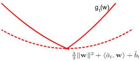
Figure 4: Quadratic underestimator of gt(w) (solid line) and corresponding aggregated cutting
plane ˜ct(w)(dash line)).
remove fromJt−1. In our implementation, we maintain a count for each CP which is the number of
iterations in which the CP does not contribute to the aggregation CP (see below for details about the definition of the aggregation CP). Then the CP with highest count is selected to be removed.
Cutting plane aggregation. The use of an aggregated cutting plane is a key issue to limit storage requirements and computational effort per iteration. The technique is inspired by the subgradient aggregation idea of Kiwiel (1983), which can be viewed as building a low cost approximation of the piece-wise quadratic function in Equation 4. Basically, by considering a linear combination of subgradient of f computed in previous iterations, we can discard previous subgradients without losing all information. In our method, we also use aggregation technique for building a low cost approximation of the approximation functiongt(w). Note that we use a slightly different
terminol-ogy (CP aggregation instead of subgradient aggregation) since our goal is to build an approximation of f using cutting planes, rather than building an approximation of subdifferential as in standard bundle methods which aims at finding a solution with small sub-gradient. There are two key differ-ences between our CP aggregation technique and the subgradient aggregation proposed originally by Kiwiel (1983). First, our method is specifically designed for quadratically regularized objective which makes possible to show that our limited memory variant using CP aggregation inherits the theoretical convergence rate of CRBM (as least for convex risks). Instead the standard subgradient aggregation technique can be applied to any objective function by using an additional regularization term in the search direction optimization problem. Second, while the original method focuses on aggregating subgradients, our algorithm applies the aggregation idea to both the direction, ˜a, and to the offset, ˜b(and also to the locality measure in the non convex case, see later in Section 3.2.4).
At iteration t of Algorithm 3, the cutting plane aggregation ˜ct(w) is derived from the
mini-mization of gt(w). We use the cutting plane technique to build an underestimator of gt(w)at its
minimum ˜wt =argminwgt(w). Although any linear combination of previous cutting planes could
yield an under estimator ofgt(w), only one of them, that we note ˜ct(w)hereafter, corresponds to a
tight quadratic approximationλ2kwk2+c˜
t(w)that reaches the same minimum asgt(w):
˜
wt =argmin
w
gt(w) =argmin
w
λ
2kwk 2+c˜
t(w).
The particular property of ˜ct(w) is important since it allows to guarantee that for the limited
Figure 4 illustrates the quadratic function (in red dash line) derived from the aggregated cutting plane at iterationt=2. The cutting plane ˜ct(w)can be defined based on the dual solution of the
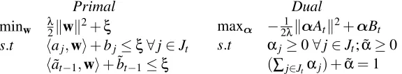
approximation problem which may be characterized in primal and dual forms as follows:
Primal Dual
minw λ2kwk2+ξ
s.t haj,wi+bj≤ξ∀j∈Jt
ha˜t−1,wi+b˜t−1≤ξ
maxα −21λkαAtk2+αBt s.t αj≥0∀j∈Jt; ˜α≥0
(∑j∈Jtαj) +α˜ =1
whereAt= [...;aj;...,a˜t−1]is a matrix (withaj and ˜at−1being row vectors),Bt = [...;bj;...; ˜bt−1]is
the vector of scalars andαstands for the (row) vector of Lagrange multipliers (of length|Jt|+1 at iterationt). We denoteαjas the Lagrange multiplier associated with the CPcj and we denote ˜αas
the Lagrange multiplier associated with the aggregated CP ˜cj−1. Letαt be the solution of the above dual program then the minimizer of the primal can be expressed as:
˜ wt=−
αtAt
λ =−
∑j∈Jtαjaj+α˜a˜t−1
λ .
The following proposition show how to useαt for defining a tight underestimator ofgt(w).
Proposition 1 Letc˜t(w) =ha˜t,wi+b˜t be the aggregated CP defined by:
˜
at =αtAt =∑j∈J
tαjaj+α˜a˜t−1,
˜
bt =αtBt =∑j∈J
tαjbj+α˜b˜t−1 then the quadratic function λ2kwk2+c˜
t(w)is an underestimator of gt(w), which reaches the same
minimum value as gt(w)at the same point,w˜t.
Proof First, by construction we have ˜wt=−a˜λt which implies that the derivative of2λkwk2+c˜t(w)
is null at ˜wt. Second, we can show that λ2kw˜tk2+c˜t(w˜t) =gt(w˜t). Actually:
gt(w˜t) =−21λkαtAtk2+αtBt =−λ 2k
˜ at
λk2+b˜t
=λ2ka˜t
λk2−λk
˜ at
λk2+b˜t =λ2kw˜tk2− ha˜t,a˜λti+b˜t
=λ2kw˜tk2+ha˜t,w˜ti+b˜t.
(12)
In other words, the quadratic function λ2kwk2+c˜
t(w)and the approximation functiongt(w)reach
the same minimum valuegt(w˜)at the same point ˜wt.
Finally, we show that λ2kwk2+c˜
t(w)is an underestimator ofgt(w). Let
ht(w) =max
max
j=∈Jt
haj,wi+bj,ha˜t−1,wi+b˜t−1
be the piecewise linear approximation ofR(w)at iterationt, we have:
0∈∂gt(w˜t)≡λw˜t+∂ht(w˜t)
since ˜wt is the optimum solution of minimizinggt(w). Note that ˜at =−λw˜t, the above equation
implies that ˜at ∈∂ht(w˜t). In other words, ˜at is a subgradient of ht(w)at ˜wt. Furthermore, since
gt(w˜t) =λ2kw˜tk2+ht(w˜t), Equation 12 gives:
The cutting plane ˜ct(w)is then an underestimator ofht(w)built at ˜wt (recall thatht(w)is convex),
and thus λ2kwk2+c˜
t(w)is a quadratic underestimator ofgt(w) = 2λkwk2+ht(w). Note that since λ
2kwk 2+c˜
t(w) is an underestimator ofgt(w) and gt(w) is an underestimator of f(w) atw∗t, the
quadratic functionλ2kwk2+c˜
t(w)is also an underestimator of f(w)atw∗t.
3.2 Regularized Bundle Method for Non-Convex Risks
To handle non-convex objective function, we introduce some new notations in addition to the nota-tion used in Algorithm 3. In the following, we recall useful notanota-tions from previous secnota-tion, and we introduce additional notations that will be useful hereafter.
Notations from limited memory CRBM.At iterationt,wt is the current solution andwt∗is the best
observed solution. Jt corresponds to the working set of cutting plane, which is involved in the
definition of the approximation gt(w). ˜wt is the solution of the minimization ofgt(w), it is also
considered as the solution in the next iteration.
Raw and modified cutting planes. We have to distinguish between a raw linear cutting plane of the riskcwj (withcwj(w) =hawj,wi+bwj) that is built at a particular iteration jof the algorithm and the
eventually modified versions of this cutting plane that might be used in posterior iterations. Indeed a cutting plane may be modified multiple times for solving conflicts as in standard NBM method. At iterationt we notectj (withctj(w) =haj,wi+btj) the cutting plane which is derived fromcwj,
the raw CP originally built at iteration j. Unlike NBM, the normal vectoraj in our algorithm might
be different than the subgradientawj computed atwj, due to our particular solving conflict method.
However, once defined at iteration j, the normal vector aj remains fixed over iterations. On the
contrary, the offset might be modified multiple times for solving conflicts occurring after iteration
j, and we use a superscripttindicating the iteration number for the cutting plane’s offsetbtj.
Bundle. The bundle Bt denotes the state of the algorithm at iteration t. It consists in a set of
cutting planes which were built at previous solutions,ctjfor j∈Jt. Similarly to non-convex bundle
methods, we define a locality measure which is associated to any active cutting plane. It is related to the locality measure between the cutting plane (actually the point where the cutting plane was built) and the best current observed solution. We notestjthe locality measure between cutting plane
ctj and the best observed solution up to iterationt,wt∗. The full bundle information is:
Bt ={ctj,stj}j∈Jt∪ {c˜
t
t−1,s˜tt−1}
where ˜ctt−1 is an aggregated cutting plane and ˜stt−1 is its locality measure to the best observed solutionw∗t. Similar to the aggregation technique presented in Section 3.1, the aggregated CP ˜ctt−1
can be viewed as a convex combination of CPs in previous iterations. For non-convex objective function, each CP in the bundle is associated with a locality measure, including the aggregated CPs whose locality measure is a convex combinations of locality measures of other CPs.
3.2.1 SKETCH OF ALGORITHM
Algorithm 4NRBM
1: Input: w1,R,λ,ε,M 2: Output: w∗
3: Initialization:
4: Compute cutting planecw1 ofR
5: [c11,s11] = [c˜11,s˜11] = [cw1,0]
6: w˜1=−a1/λ
7: B1={c11,s11,c˜11,s˜11}
8: fort=2 to∞do
9: wt←w˜t−1
10: Compute cutting planecwt ofR
11: w∗t =argminw∈{w1,...wt}f(w)
12: Bt = UpdateBundle(Bt−1,w∗t−1,w∗t,cwt,wt,M) 13: (w˜t,c˜tt,s˜tt)= MinimizeApproximationProblem(Bt,λ)
14: gapt= f(w∗t)−gt(w˜t)
15: ifgapt<εthen return wt∗
16: end for
Similar to CRBM and limited memory CRBM, the approximation problem is designed in such a way that one can use the minimum of the approximation problem as the new current solution. In other words, NRBM does not require a dedicated line search procedure to ensure convergence as in the standard NBM (Kiwiel, 1985). Such a line search is not required for convergence matters in our method but it may be still used for improving convergence rate in practice (see Section 3.3.2).
Initialization
Initialization consists in providing a first bundle B1. Starting with an initial solutionw1, we build the first cutting planec11=cw1 =haw1,wi+bw1. Note that at iterationt=1, there is only one cutting planec11 and the aggregated cutting plane is alsoc11: [c˜11,s˜11] = [c11,s11]. Theapproximation functionis then:
g1(w) =λ 2kwk
2+ha
1,wi+b11
which reaches its minimum at ˜w1=−a1/λ. The state of algorithm B1 is set to c11 and ˜c11 (which coincide) with their corresponding locality mesures to the best solutionw1( ˜s11=s11=0).
Iterationt
Every iteration the algorithm determine a new bundle Bt, the best observed solution up to
it-erationt, w∗t, and the new current (and temporary) solutionwt. At iterationt>1, few steps are
successively performed:
• Build a new cutting plane at ˜wt−1the minimizer of approximation function in previous itera-tion (gt−1(w)).
• Update the best observed solutionw∗t.
• Solve any conflict between the best observed solution,wt∗, and all cutting planes in the bundle. This is done through a call to UpdateBundle function which we detail later. This yields a piece-wise quadratic functiongt which is a local underestimator approximation of f. As said
special aggregated cutting plane, ˜ctt−1for gathering information of previous cutting planes up to iterationt−1. The approximation function at iterationtis then:
gt(w) = λ
2kwk
2+max
max
j∈Jt
ctj(w),c˜tt−1(w)
(13)
where, as in Section 3.1,Jt stands for a subset of cutting planes defined in previous iterations
if one wishes to use a limited memory variant.
• Minimizegt. This gives a solution named ˜wt which will be used in next iteration. Note that
a side effect of this minimization is the definition of a new aggregated cutting plane and its locality measure to the best observed solutions.
This procedure is repeated until the gap (i.e. the difference between the best observed value of objective function and the minimum of the approximation function) is less than a desired accuracy
ε. We say that anε-solution has been reached.
We detail in the following sections how the approximation is built and procedure for solving conflict in the update of the bundle. Then we provide details on our definition of the aggregated cutting plane.
3.2.2 LOCALITYMEASURE ANDCONDITIONS ONCPS
Given a set of cutting plane approximation ofR, one could build a local underestimator of f in the vicinity ofwby descending CPs that yields non positive linearization error of f atw. Our algorithm focus on solving conflicts between CPs in the bundle and the best observed solutionw∗t. While sharing some concepts with NBM such as locality measure, null step and descent step our method is based on a new greedy strategy for solving conflicts which guarantee a minimum improvement of the approximation gap after each iteration which is similar to CRBM.5
Locality measure definition. We propose to define the locality measure between a cutting plane previously built at iteration jand the current best solutionw∗t based on the trajectory fromwjtow∗t.
We exploit the same shape of our regularization term (L2 norm) to define our locality measure.6 At iterationt, we define the locality measure between CPctjbuilt atwjandwt∗as:
stj=s(wj,w∗t) = λ
2 kwj−w ∗
jk2+ t
∑
k=j+1
kw∗k−w∗k−1k2
!
which yields a natural recursive formulate:
stj=stj−1+λ 2kw
∗
t −w∗t−1k2,∀j<t.
Lower bound and upper bound on offset adjustment.As in NBM, raw CP cannot always be used to build an underestimator of f(w), which is non-convex so that CP need adjustments. We discuss two conditions that define an upper and an underestimator on a CP’s offset modification when solving a conflict with respect tow∗t.
5. Note that we use the terminology descent step instead of serious steps since descent step here is not fully similar to serious step in standard non convex bundle methods.
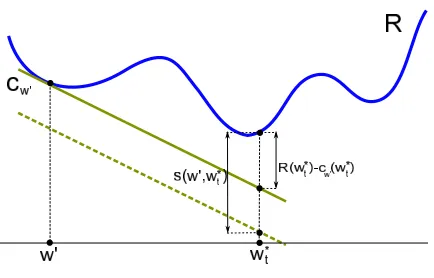
Figure 5: Conflict betweenw∗t and a cutting planecw′.
First, as in standard NBM (recall Equation 10), we consider the following firstcondition requir-ing that a CP built atw′,cw′, gives a positive linearization error atw∗t, which must grow with the
locality measure of the CP tow∗t:
R(wt∗)−c(wt∗)≥s(w′,w∗t) (14) where s(., .) is our non-negative locality measure between the two points. The positive value of
s(w′,wt∗)ensures that the linear approximationcw′(w)is an underestimator ofR(w)at least within
a small region aroundw∗t. Figure 5 illustrates this case. The cutting planecw′ which was built atw′
does not satisfy condition 14. This conflict between cutting planecw′ andw∗t is solved in NBM by
loweringcw′(by tuning its offsetb′) so that the linearization error atwt∗,R(wt∗)−cw′(wt∗), becomes
at leasts(w′,wt∗). This yield anupper boundon the new offsetb′:
b′≤R(w∗t)− ha′,w∗ti −s(w′,w∗t). (15) Unfortunately if a cutting plane is lowered too much, the minimum of the approximation func-tion is not guaranteed to improve every iterafunc-tion anymore. For instance it may happen that the minimum of the approximated function is not changed once the new cutting plane has been low-ered, yielding a infinite loop without any improvement on the solution. Standard non-convex bundle methods handle this problem with a special line search procedure (between the current best observed solution and the minimum of the approximation problem) with stopping conditions that ensure some minimal changes of the approximation problem.
We found instead that there is a simple sufficient condition that guarantees an improvement of the minimum of the approximation function every iteration (required by Lemma 4). It concerns the new added cutting plane only and writes: λ2kwtk2+hat,wti+btt ≥f(wt∗). In other words, we need
to ensure that the approximation atwt using the new added cutting plane is greater or equal to the
best observed function value. Note thatwt is the minimizer of the approximation in the previous
iteration, gt−1(w), this condition influences directly the gap between the best observed function value and the minimum of the approximation. The condition can be seen as a lower bound on the modified offset:
btt≥ f(w∗t)−λ
2kwtk 2− ha
Algorithm 5UpdateBundle
1: Input:Bt−1={ctj−1,stj−1}j∈Jt−1∪ {c˜
t−1
t−1,s˜tt−1−1},w∗t−1,w∗t,wt,cwt,M 2: Output:Bt={ctj,stj}j∈Jt∪ {c˜
t
t−1,s˜tt−1}
3: if wt∗6=w∗t−1then Descent Step
4: for j∈Jt−1
5: stj=stj−1+2λkwt∗−w∗t−1k2
6: btj=min[btj−1,R(w∗t)− haj,w∗ti −stj]
7: end
8: s˜tt−1=s˜tt−1−1+λ2kw∗t −wt∗−1k2
9: b˜tt−1=min[b˜tt−1−1,R(wt∗)− ha˜t−1,wt∗i −s˜tt−1]
10: c˜tt−1(w):=ha˜t−1,wi+b˜tt−1
11: [ctt,stt] = [cwt,0]
12: else Null Step
13: for j∈Jt−1
14: ctj=ctj−1;stj=stj−1;
15: end
16: c˜tt−1=c˜tt−1−1; ˜stt−1=s˜tt−1−1;
17: ifcondition (15) is not satisfied forcwt then 18: [ctt,stt]= SolveConflictNullStep(w∗t,wt,cwt) 19: else[ctt,stt] = [cwt,
λ
2kwt−wt∗k2]
20: end
21: Jt =UpdateWorkingSet(Jt−1,t,M)
22: returnBt ={ctj,stj}j∈Jt} ∪ {c˜
t
t−1,s˜tt−1}
3.2.3 BUNDLEUPDATE
The approximation function,gt, is refined every iteration, Algorithm 5 describes theU pdateBundle
process. It takes as input:
• The bundle at previous iteration
• The best observed solutions at previous iterationw∗t−1
• The best observed solutions at current iterationwt∗
• The current solutionwt and its corresponding raw cutting plane,cwt.
The algorithm is designed so that at the end of iteration t, all (|Jt|+1) cutting planes in the
bundle (i.e. the|Jt|“normal” cutting planes and the aggregated cutting plane) satisfy condition in
Equation 15 while the new added cutting planectt also satisfies condition in Equation 16. Note that
cwt always satisfies (16) by definition ofw
∗
t, so thatctt also satisfies (16) in case there is no conflict
(ctt ≡cwt).
As the two conditions (15) and (16) involve the best observed solution, we distinguish two cases when solving conflict. Either the current solution is the best solution up to now (hencew∗t 6=wt∗−1), in which case we call the iteration a descent step. Or the current solution is not the best solution (i.e. w∗t ≡w∗t−1), then the iteration is said to be a null step. We detail these two cases now.
Descent Step. In the case of a descent step, condition (16) is trivially satisfied for the new added cutting plane sincect
t ≡cwt. Hence solving an eventual conflict is rather simple in this case. It is
done by setting:
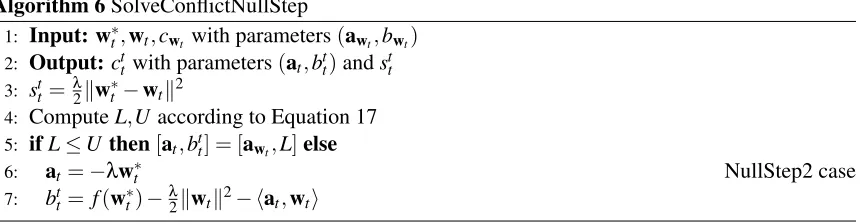
Algorithm 6SolveConflictNullStep
1: Input: w∗t,wt,cwt with parameters(awt,bwt) 2: Output:ctt with parameters(at,btt)andstt
3: stt= λ2kw∗t −wtk2
4: ComputeL,Uaccording to Equation 17
5: ifL≤U then[at,btt] = [awt,L]else
6: at=−λw∗t NullStep2 case
7: btt= f(w∗t)−2λkwtk2− hat,wti
for all jin the working set. A similar modification may be applied to the aggregated cutting plane:
˜
btt−1=min[b˜t−1
t−1,R(w∗t)− ha˜t−1,w∗ti −s˜tt−1]
where ˜stt−1=s˜t−1+λ2kwt∗−wt∗−1k2. At the end, the adjusted aggregated CP (in the working set of iterationt) is:
˜
ctt−1(w) =ha˜t−1,wi+b˜tt−1.
Null Step.In the case of a null step, the best observed solution did not change, so thatstj=stj−1,∀j= 1, ...,(t−1)and ˜stt−1=s˜tt−1−1. Since all cutting planes inBt−1were already adjusted to satisfy positive linearization error condition wrt. the best solution at previous iteration, a conflict (if any) may only arise between the new cutting planecwt and the best observed solutionw
∗
t. So that all CPs (including
aggregated CP) remain unchanged (see Algorithm 5 line 13) except the new added CP which must be checked for conflict.
In the null step case, solving conflict is not as simple as in a descent step case since as we said before, for convergence proof matters, we need the new cutting plane to satisfy both conditions (15) and (16). Algorithm 6 modifiesctt in such a way that it guarantees that the new cutting planectt with parametersat andbtt satisfies conditions (15) and (16). In a first attempt it tries to solve the conflict
by tuningbtt alone while fixingat =awt. Indeed conditions (15) and (16) may be rewritten as:
btt ≤R(w∗t)− hawt,w∗ti −stt =U,
btt ≥ f(w∗t)−λ2kwtk2− hawt,wti=L
(17)
which define an upper boundUand a lower boundLforbtt. IfL≤U any value in(L,U)works (in our implementation we setbtt =L).
However it may happen thatL>U, then tuningbttis not enough (this is what we call a NullStep2 case in Algorithm 6). Bothbtt and the normal vectorat need to be adjusted to make sure that the
conflict is solved (see Line 6 in Algorithm 6).
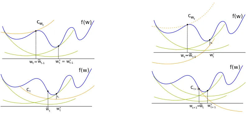
Figure 6(top-left) illustrates an example of NullStep2 where the gradient information given atwt
is not helpful for building a local underestimator approximation atw∗t. The quadratic approximation corresponding to cutting planecwt is plotted in orange, which is not a local underestimator of f(w)
atwt∗. The conflict is so severe that it cannot be solved by just lowering the cutting plane. It should be lowered too much with respect to condition in Equation 15 (Figure 6 (top-right)), meaning that the approximation function would be unchanged and the algorithm would loop without finding a good solution.
In a NullStep2 case, we propose to ignore the gradient information atwt and to rather focus on
Figure 6: Illustration of NullStep2. Top-left: conflict arise at iterationt. Top-right: can not solve conflict by descend the cutting plane. Bottom-left: Nullstep2, modifying the cutting plane to solve the conflict at iterationt. Bottom-right: There is no conflict at iterationt+1.
local underestimator, λ2kwk2+ha
t,wi+btt) satisfying both conditions in Equation 15 and 16). This
quadratic function is defined so that it reaches its minimum atwt∗and the linearization error of the cutting planehat,wi+btt atw∗t is λ2kwt−w
∗
tk2(see the orange quadratic curve in Figure 6
(bottom-left)). The new cutting plane is defined as:
ctt(w) =hat,wi+btt,
at =−λwt∗,
btt = f(wt∗)−λ2kwtk2− hat,wti,
stt =λ2kwt−w∗tk2.
This CP satisfies condition (16) by construction. It also satisfies condition (15) as we show now:
hat,w∗ti+btt =hat,wt∗i+f(wt∗)−λ2kwtk2− hat,wti =R(wt∗) +hat,w∗t −wti+λ2(kwt∗k2− kwtk2)
=R(wt∗) +hat+λ2(wt∗+wt),w∗t −wti
where we used the definition of the objective function f(wt∗) = λ2kw∗tk2+R(w∗
t). Then, substituting
−λwt∗forat (Cf. Line 6) we obtain:
hat,w∗ti+btt =R(w∗t)−λ2kw ∗
t −wtk2
⇐⇒ hat,w∗ti+btt =R(w∗t)−stt
⇐⇒ btt =R(w∗t)− hat,w∗ti −λ2kw∗t −wtk2
Figure 7: Quadratic underestimator ofgt(w)derived from the aggregated cutting plane ˜ctt(w).
3.2.4 APPROXIMATED PROBLEM AND AGGREGATED CUTTING PLANE
In the non-convex case the aggregated CP is still an underestimator of approximation problem. Figure 7 illustrates the quadratic function (in orange) derived from the aggregated cutting plane at iterationt=2.
Solving the approximated problem and definition of the aggregated cutting plane are completely similar to the case of limited memory CRBM, with the only difference that we use here at iteration
tthe bundle at iterationt that may include cutting planes that have been modified during previous iterations.The minimization of the approximation function (gt(w)in Equation 13) can be solved in
the dual space as:
Primal Dual
minw λ2kwk2+ξ
s.t hatj,wi+btj≤ξ∀j∈Jt
ha˜tt−1,wi+b˜tt−1≤ξ
maxα − 1
2λkαAtk2+αBt s.t αj≥0∀j∈Jt; ˜α≥0
(∑j∈tJtαj) +α˜ =1
whereAt= [...;atj;...; ˜att−1]is a matrix (withatj and ˜att−1being row vectors),Bt = [...;btj;...; ˜btt−1]is the vector of scalars andαstands for the (row) vector of Lagrange multipliers (of length|Jt|+1 at iterationt). We denoteαjas the Lagrange multiplier associated with the CPctj and we denote ˜αas
the Lagrange multiplier associated with the aggregated CP ˜ctj−1. Letαt be the solution of the above dual program then the minimizer of the primal can be expressed as:
˜ wt =−
αtAt
λ .
Hence the definition of the aggregated cutting plane follows:
˜
at =αtAt, ˜
bt =αtBt.
Locality measure associated to the aggregated cutting plane.The aggregated CP ˜ctt accumulates in-formation from many cutting planes built at different points so that one cannot immediately define a locality measure ˜stt between ˜ctt and the current best observed solutionwt∗. However, ˜ctt being a con-vex combination of cutting planes, we chose to define ˜st
t as the corresponding convex combination
of locality measures associated to cutting planes:
˜
stt =
∑
j∈Jt
Interestingly using this aggregated locality measure, one can show that there is no conflict between ˜
ctt andw∗t sinceR(w∗t)−c˜tt(wt∗)≥s˜tt. Indeed, we have:
R(w∗t)−ctj(w∗t) ≥stj∀j∈Jt,
R(w∗t)−c˜tt−1(w∗t) ≥s˜tt−1.
Multiplying these equations byαj’s and ˜αthen taking the sum gives the result:
R(wt∗)−c˜tt(w∗t)≥s˜tt.
3.3 Variants
In this section we discuss two variants (and their implementations issues) that allow speeding up convergence in practice.
3.3.1 REGULARIZATION
In previous section we presented our method with a standard L2 regularization term λ2kwk2. Yet this choice is not always a good one for non-convex optimization problems where convergence to a poor local optima is a severe problem. Alternatively one may prefer to regularize around a first reasonable solutionwreg and use a regularization term such ask(w−wreg)k2. For instance to learn Hidden Markov Models with a large margin criterion using a variant of NRBM, we used a model learned with Maximum Likelihood aswreg(Do and Arti`eres, 2009). Furthermore, if all parameters
inwdo not have the same nature (magnitude) then using only one weight-cost (λ) for all parameters is not wise. So one may prefer the following regularization term:
λ
2k(w−w
reg)⊗θk2
whereθis a positive vector of regularization weights and⊗stands for element-wise product. The use of differentθvalues depending on the parameters allows introducing some prior information. Again, taking our example of learning Hidden Markov Models, we used different θ values for regularizing transition probabilities and emission probabilities parameters.
3.3.2 FASTVARIANT WITHLINESEARCH
In Algorithm 4, the minimum point of the approximation function is not guaranteed to be a better solution than the current best observed solution, which may result in null steps. Few works showed that one can speed up cutting plane based methods with a linesearch procedure (Franc and Sonnen-burg, 2008; Do and Arti`eres, 2008), which may be efficient to compute in some cases (e.g. primal objective of linear SVM).
The idea is that a line search ensures that we get a better solution every iteration, assuming that the search direction is a descent direction. If the search direction is not a descent direction then the line search returns the best solution along the search direction (should be close to the current solution), which will be used to build a new cutting plane in the next iteration. In our case, without specific knowledge of f(w)we use a general line search technique.