Published online February 2, 2015 (http://www.sciencepublishinggroup.com/j/acm) doi: 10.11648/j.acm.20150401.14
ISSN: 2328-5605 (Print); ISSN: 2328-5613 (Online)
Optimal Harvesting Policy of Discrete-Time Predator-Prey
Dynamic System with Holling Type-IV Functional Response
and Its Simulation
Rui-Ling Zhang, Wan-Xiong Wang
*, Li-Juan Qin
College of Resources and Environmental Science, Gansu Agricultural University, Gansu 730070, PR China
Email address:
[email protected] (Rui-Ling Zhang), [email protected] (Wan-Xiong Wang)
To cite this article:
Rui-Ling Zhang, Wan-Xiong Wang, Li-Juan Qin. Optimal Harvesting Policy of Discrete-Time Predator-Prey Dynamic System with Holling Type-IV Functional Response and Its Simulation. Applied and Computational Mathematics. Vol. 4, No. 1, 2015, pp. 20-29.
doi: 10.11648/j.acm.20150401.14
Abstract:
This paper deals with a discrete-time prey-predator system with Holling type-IV function response in the presence of some alternative food to predator and harvesting of prey species. By theoretical analysis and numerical simulation, comparing with the system without harvesting, ecological equilibrium point of the system is removed if harvesting effort is changed, and the appropriate harvesting effort can increase the stability of the system. Moreover, optimal harvesting policy is obtained using Pontryagin’s maximum principle. Meanwhile, some numerical simulations verify our analytical results. This study also gains the maximum economic profit which is based on the ecological equilibrium. The suitable price of resources can control the excessive harvest to promote the sustainable development of species.Keywords:
Discrete-Time Predator-Prey Model, Equilibrium, Pontryagin Maximum Principle, Bifurcation, Sustainable Development1. Introduction
More and more importance has been attached to human concerning ecology and environment as a result of population growth, environmental pollution, resource depletion and other serious social problems. In recent years, the optimal management of renewable resources has a close connection with the sustainable development of population systems and the profit of the owners, in which ecologists and economists are very interested. And there is a lot of literature on this topic. An excellent introduction of the optimal management of renewable resources has been given[1]. It has been gotten some nice generalizations about the problems of continuity predator-prey system, and the optimal harvesting policy applied to the development and utilization of resources and the protection of species [2-4]. It is possible to prevent species damage or extinction by an appropriate planning in proper time [5].
The discrete-time model has more practical meaning for the species short-lived and time without overlapping [6]. Many studies also focus on the discrete model of the optimal harvesting problem [7-8]. Arino et al. (2001) suggested that the
time delay to adulthood should be state dependent and careful formulation of such state dependent time delays can lead to models that produce periodic solutions. Gourley & Kuang (2004) formulated a general and robust prey-predator model with stage-structure with constant maturation time delay and performed a systematic mathematical and computational study. They have shown that there is a window in maturation time delay parameter that generates sustainable oscillatory dynamics. Sadhukhan et al. (2008) studies a discrete age-structured BLL population model with age dependent harvesting and its stability. Eduardo & Pawel (2012) showed that a comprehensive overview of the dynamics as the harvest rate and survival probability change and the range of parameters for population abundance get larger in spite of an increase in the harvest rate in a stage-structured discrete population. Raghib et al. (2013) discussed the dynamics of population models under the effect of constant yield harvesting and showed that some regions of persistence and characterize of extinction. Ghosh & Kar (2014) deal with a prey-predator system in the presence of some alternative food to predator and harvesting of prey species.
Dawkins & Krebs (1979), Qi Jun & Su Zhiyong (2011) studied a predator-prey system with Holling type III and prey with positive effect. The model is expressed as follow:
0
(1 ) ( )
( ) .
N P
dN
rN N P
dT K
dP
b N P mP
dT α ϕ ϕ − = − − = − , (1)
where N is the density of prey, P is the density of predators, T is time. α0 is a positive adjustment factor of
predator populations to prey populations (expressing that idle resources can be released for survival after each predator hunt for food, prey population could reproduce α0 individual prey). The predator possesses a constant per capita mortality rate m, consumes the prey with Holling type-IV functional response ϕ( )N , and converts consumed prey into new predators with efficiency b. In the absence of predator, the prey grows logistically with intrinsic rate of growth r and carrying capacity K. Nand Pare nonnegative variables;
r, b, Kand m are positive parameters.
The former work shows the influence of equilibrium and dynamic evolution on the system with positive effect for prey. First,the increase of positive effect has strengthen the
stability of the system,while more increase in the defensive
ability of prey would lead to the change of the system stability, finally it made both the predator and prey go towards the infinite and our system collapsed. Meanwhile, they gain the result of three equilibrium points (equilibrium (0, 0), a boundary equilibrium point, a positive equilibrium point) in their paper. In this study, we discuss a dynamic reaction model of a prey-predator system with Holling type-IV function response, and consider that the prey species is subject to harvesting from two aspects of theory analysis and numerical simulation, which is based on the model (1).
2. The Establishment of Model
In 1930, Haldance introduced Holling type-IV function response in enzymology, and it was then used in many
studies[18-19], which takes form as follows: ( ) 2
t t
t t
cN N
N i N a
ϕ =
+ + ,
where c i a, , are positive parameters. The parameters c and
a can be interpreted as the maximum per capita predation rate and the half-saturation constant in the absence of any inhibitory effect. The parameter i, in turn, is a direct measure of the predator’s immunity from, or tolerance of, the prey.
Harvesting policy is formulated by catch-per-unit-effect hypothesis (Clark, 1990) and presented as h N E( , )=qEN , whereqis the catch ability coefficient and Eis the harvesting effort. However, it is important to note that effect (i.e., reaper, equipment and other instruments) also act as the predator. If the handing time is taken into account to catch the prey species, then the above unrealistic features can largely be removed by adopting the alternative functional form[20] h N E( , ) qEN
dE LN =
+ ,
where d is the degree of competition among the business of harvest, L is the product of harvest rate and handing time.
The system (1) is processed with the discrete way using Euler method. We can rewrite the system (1) by the harvesting rule and Holling type-IV function response, the new model as following:
0
(1 ) ( ) ,
1
( ) .
1
Nt Pt qENt
Nt Nt rNt N Pt t
K dE LNt
Pt P bt N P mPt t t
α ϕ ϕ − = + − − − + + = + − + (2)
The ecological meaning of parameters is the same as above.
3. The Stability Analysis of Model
We just analysis it in the first quadrant for making the system (2) have the ecological significance, After some calculations, we have the equilibrium points which is listed in Table 1, along with conditions for their existence. At E0, both
species are extinct. At E1 and E2, the prey is at its carrying
capacity and the predator is extinct. Finally, at E3 and E4,
the predator and prey coexist.
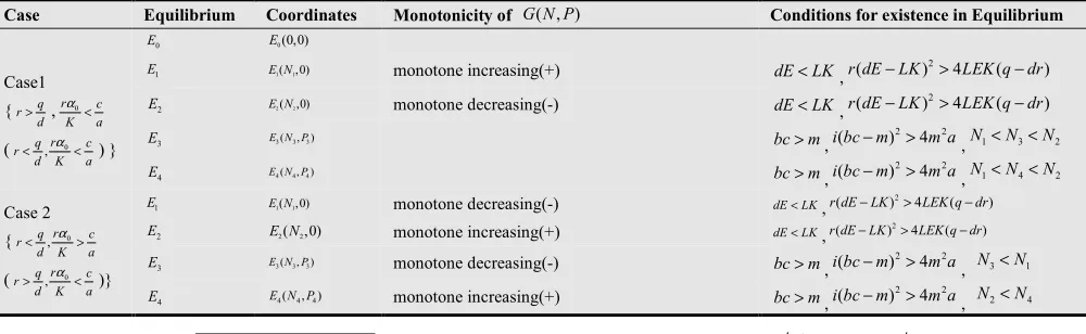
Table 1. Equilibria
Case Equilibrium Coordinates Monotonicity of G N P( , ) Conditions for existence in Equilibrium
0
E E0(0,0)
Case1
{r q d > ,r 0 c
K a α < ( 0 ,r q c r
d K a α < < ) }
1
E E N1( 1,0) monotone increasing(+) dE<LK,
2
( ) 4 ( )
r dE−LK > LEK q−dr
2
E E N2( 2,0) monotone decreasing(-) dE<LK
,
2
( ) 4 ( )
r dE−LK > LEK q−dr
3
E E N P3( 3,3) bc>m
,
2 2
( ) 4
i bc−m > m a,N1<N3<N2
4
E E N P4( 4,4) bc>m,
2 2
( ) 4
i bc−m > m a,N1<N4<N2
Case 2
{ 0
,r
q c
r
d K a α < > ( 0 ,r q c r
d K a α > < )}
1
E E N1( 1,0) monotone decreasing(-) dE<LK,
2
( ) 4 ( )
r dE−LK > LEK q−dr
2
E E N2( 2,0) monotone increasing(+) dE<LK,
2
( ) 4 ( )
r dE−LK > LEK q−dr
3
E E N P3( 3,3) monotone decreasing(-) bc>m
,
2 2
( ) 4
i bc−m > m a, N3<N1
4
E E N P4( 4, 4) monotone increasing(+) bc>m,
2 2
( ) 4
i bc−m > m a, N2<N4
(Note:
2 1 2
( ) ( ) 4 ( )
,
2
dEr LKr dEr LKr LrEK q dr N N
Lr
− − ± − − −
= , 2 2
3, 4 [( ) ( ) 4 ]
2
i
N N bc m bc m m a i m
= − ± − − , 3 2 3 3
3 3 0
( ( ) )
( )
r qE dE LN N r K P
c N i N a αr K
− + −
=
+ + − ,
4 4
4 2
4 4 0
( ( ) )
( )
r qE dE LN N r K P
c N i N a αr K
− + −
=
+ + − , ( , ) (1 0 ) 2
N P c qE
G N P r P
K N i N a dE LN
α
−
= − − −
Next, we judge the stability of the five equilibrium points according to the theory from X.Liu & D.Xiao (2007) and Zheng B.D. (2010)[21-22].
Lemma 1 As for 2
( ) ,
F λ =λ +Bλ+C if F(1)>0, λ1and
2
λ are roots of F( )λ =0, then
(i) λ1 <1,λ2 <1if and only if F( 1)− >0,C<1;
(ii) λ1 <1,λ2 >1 ( λ1 >1,λ2 <1 ) if and only if
( 1) 0
F − < ;
(iii) λ1 >1,λ2 >1 if and only if F( 1)− >0,C<1;
To community matrixJ, if λ1,λ2 are eigenvalues of the
corresponding characteristic equation. Equilibrium point is a sink point, and asymptotically stable when λ1 <1,λ2 <1.
Equilibrium point is a saddle point when
1 1, 2 1
λ < λ > ( λ1 >1,λ2 <1). It is an unstable source point
when λ1>1,λ2 >1.
Lemma 2 λ1<1,λ2 <1if and only if
3 3
1−tr J( ) det+ J >0,1+tr J( 3) det+ J3 >0, det J3 <1.
The corresponding community matrix to system (2) is as follow:
2 2
2 0 (( ) (2 1)) 0
1 (1 )
2 2 2 2
( ) ( )
2
(( ) (2 1))
1
2 2 2
( )
N P cP N i N a N N i qdE r N cN r
K N i N a dE LN K N i N a
J
cPb N i N a N N i bcN
m
N i N a N i N a
α α − + + − + + − − − − + + + + + = + + − + + − + + + +
At equilibrium point E0, the corresponding community
matrix is as following:
0 1 0 0 1 q r J d m + − = − ,
the eigenvalues are 1 1
q r
d
λ = + − , λ = −2 1 m. The nature of
equilibrium point E0(0, 0) is discussed by the following
aspects:
(i) E0(0, 0) acts as a stable sink point while r q r 2
d < < +
and 0< <m 2.
(ii) E0(0, 0) is a saddle point and the system (2) is unstable whiler q
d
> (r q 2
d
< − ),0< <m 2 or r q r 2
d
< < + ,m>2.
(iii) E0(0, 0) is an unstable source point for r q d
> (r q 2
d < − )
and m>2.
In order to investigate the nature of the two boundary equilibrium, we take separately equilibrium point E N1( 1, 0)
and E N2( 2, 0) into equation (3). The community matrix to
1( 1, 0)
E N is as follow:
2
0 1
1 1
2 2
1 1 1
1
1 2
1 1
2
1 (1 )
( )
0 1
r N
N qdE cN
r
K dE LN K N i N a J
bcN m N i N a
α + − − − + + + = + − + + .
The eigenvalues are 1 2
1 2
1
2
1 (1 )
( )
N qdE r
K dE LN
λ = + − −
+ ,
1
2 2
1 1
1 bcN m
N i N a
λ = + −
+ + .
Similarly, the corresponding matrix aboutE N2( 2, 0)is
2
0 2
2 2
2 2
2 2 2
2
2 2
2 2
2
1 (1 )
( )
0 1
r N
N qdE cN
r
K dE LN K N i N a J
bcN m N i N a
α + − − − + + + = + − + + .
The eigenvalues are
2 2
1 2
2
2
1 (1 )
( )
N qdE
r
K dE LN
λ = + − −
+ ,
2
2 2
2 2
1 bcN m
N i N a
λ = + −
+ + , respectively.
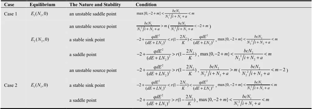
Therefore, the nature of the two boundary equilibrium can be concluded by means of Lemma 1 (see Tab. 2).
Table 2. The nature of the boundary equilibrium E1 and E2
Case Equilibrium The Nature and Stability Condition
Case 1 E N1( 1, 0) an unstable saddle point
1 2
1 1
max{0, 2 m} bcN m
N i N a
− + < + + <
an unstable source point 1
2
1 1
bcN m N i+N+a> (
1 2 1 1 2 bcN m N i+N+a< − + )
2( 2, 0)
E N a stable sink point
2 2
2
2 2
2 2
2
2 (1 )
( ) ( )
N
qdE qdE
r
dE LN K dE LN
− + < − <
+ + ,
2 2
2 2
max{0, 2 m} bcN m
N i N a
− + < <
+ +
a saddle point
2
2 2
2
2
2 (1 )
( )
N qdE
r
dE LN K
− + > −
+ ,
2 2
2 2
max{0, 2 m} bcN m
N i N a
− + < < + +
an unstable source point
2
2 2
2
2
2 (1 )
( )
N qdE
r
dE LN K
− + > −
+ , 2 2 2 2 bcN m N i+N +a> (
2 2 2 2 2 bcN m N i+N +a< − )
Case 2 E N1( 1, 0) a stable sink point
2 2
1
2 2
1 1
2
2 (1 )
( ) ( )
N
qdE qdE
r
dE LN K dE LN
− + < − <
+ + ,
1 2
1 1
max{0, 2 m} bcN m
N i N a
− + < <
+ +
a saddle point
2
1 2
1
2
2 (1 )
( )
N qdE
r
dE LN K
− + > −
+ ,
1 2
1 1
max{0, 2 m} bcN m
N i N a
Case Equilibrium The Nature and Stability Condition
an unstable source point
2
1 2 1
2
2 (1 )
( )
N qdE
r dE LN K
− + > −
+ , 1 2 1 1 bcN m N i+N+a> (
1 2 1 1 2 bcN m N i+N+a< − )
2( 2, 0)
E N an unstable saddle point 2
2
2 2
max{0, 2 m} bcN m
N i N a
− + < <
+ +
s an unstable source point 2
2
2 2
bcN m N i+N +a> (
2 2 2 2 2 bcN m N i+N +a< − + )
(Note: Case 1 is the condition ofr q
d > ,r 0 c
K a
α < (r q d < ,r 0 c
K a
α < ); Case 2 is the condition ofr q d < ,r 0 c
K a
α > (r q d > ,r 0 c
K a
α < ) )
From Table 2, we get the following conclusion (see Th.1). Theorem 1 The boundary equilibrium E1 is asymptotically
stable if and only ifr q d < ,r 0 c
K a
α >
(r q d
> ,r 0 c
K a α < ), 2 2 1 2 2 1 1 2
2 (1 )
( ) ( )
N
qdE qdE
r K
dE LN dE LN
− + < − <
+ + ,
1 2
1 1
max{0, 2 m} bcN m
N i N a
− + < <
+ + .
The equilibrium point E2 is asymptotically stable if and
only ifr q d > ,r 0 c
K a
α <
(r q d < ,r 0 c
K a α < ), 2 2 2 2 2 2 2 2
2 (1 )
( ) ( )
N
qdE qdE
r K
dE LN dE LN
− + < − <
+ + ,
2 2
2 2
max{0, 2 m} bcN m
N i N a
− + < <
+ + .
Similarly, we get the community matrix of corresponding equilibrium point E3 is
'
3 3 2 3
3
3 3 3
1 ( , ) ( )
( ) 1
G N P f N
J
f N P
+
=
. (4)
Where
2 2
' 3 0 3 3 3
3 3 2 2 2
3 3 3
2 ( )
( , ) (1 )
( ) ( )
N P cP a N i qdE G N P r
K N i N a dE LN
α
− −
= − − −
+ + + ,
0 3 3
2 3 2
3 3
( ) r N cN
f N
K N i N a
α
= −
+ + ,
2 3
3 3 2 2
3 3
( )
( )
( )
cb a N i
f N
N i N a
− =
+ + . Its trace
and determinant are '
3 3 3
( ) 2 ( , )
tr J = +G N P ,
'
3 3 3 2 3 3 3 3
det J = +1 G N P( , )−f N( )f N P( ) .
The community matrix of equilibrium point E4 is
'
4 4 2 4
4
3 4 4
1 ( , ) ( )
( ) 1
G N P f N
J
f N P
+
=
. (5)
And the corresponding characteristic equation is
2 ' '
2 3 4
( ) (2 ) 1 0
F λ =λ − +G λ+ + −G f f P = .
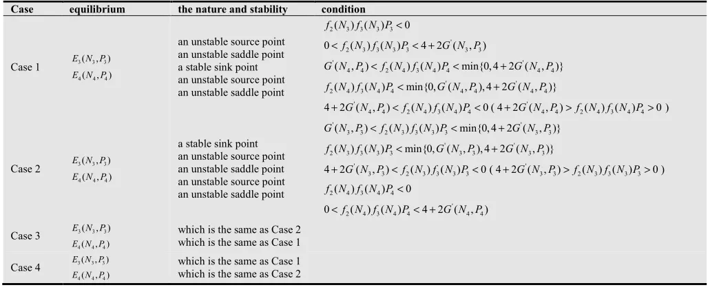
Based on Table1, Lemma 1 and Lemma 2, we get the stability of equilibrium point E3 andE4 as following (see Tab.3)
Table 3. The nature and stability of the positive equilibrium E and3 E 4
Case equilibrium the nature and stability condition
Case 1 E N P3( 3,3)
4( 4, 4) E N P
an unstable source point an unstable saddle point a stable sink point an unstable source point an unstable saddle point
2( 3) (3 3) 3 0
f N f N P<
'
2 3 3 3 3 3 3
0<f N( ) (f N P) < +4 2G N P( , )
' '
4 4 2 4 3 4 4 4 4
( , ) ( ) ( ) min{0, 4 2 ( , )}
G N P <f N f N P< + G N P
' '
2( 4) 3( 4) 4<min{0, ( 4, 4), 4+2 ( 4, 4)}
f N f N P G N P G N P
'
4 4 2 4 3 4 4
4+2G N P( , )<f N( ) (f N P) <0( '
4 4 2 4 3 4 4
4+2G N P( , )>f N( )f N P( ) >0)
Case 2 E N P3( 3,3)
4( 4, 4) E N P
a stable sink point an unstable source point an unstable saddle point an unstable source point an unstable saddle point
' '
3 3 2 3 3 3 3 3 3
( , ) ( ) ( ) min{0, 4 2 ( , )}
G N P <f N f N P< + G N P
' '
2( 3) 3( 3) 3 min{0, ( 3, 3), 4 2 ( 3, 3)}
f N f N P< G N P + G N P
'
3 3 2 3 3 3 3
4+2G N P( , )<f N( )f N P( ) <0( '
3 3 2 3 3 3 3
4+2G N P( , )>f N( )f N P( ) >0)
2( 4) 3( 4) 4 0
f N f N P<
'
2 4 3 4 4 4 4
0<f N( )f N P( ) < +4 2G N P( , )
Case 3 E N P3( 3,3)
4( 4, 4)
E N P
which is the same as Case 2 which is the same as Case 1
Case 4 E N P3( 3, 3) 4( 4, 4)
E N P
which is the same as Case 1 which is the same as Case 2
(Note: Case 1 is forr q
d
> , r 0 c
K a
α <
(r q
d
< ,r 0 c
K a
α <
), N1<N3<N5<N4<N2 ; Case 2 is for
q r
d
< , r 0 c
K a
α >
(r q
d
> , r 0 c
K a
α <
); Case 3 is
forr q
d
> ,r 0 c
K a
α <
(r q
d
< ,r 0 c
K a
α <
), N5<N N3, 4<N2; Case 4 is for
q r
d
> ,r 0 c
K a
α <
(r q
d
< ,r 0 c
K a
α <
), N1<N N3, 4<N5.
Wheremax{ ( , )G N P =0,N∈(N N1, 2)}=G N P( 5, 5))
Furthermore, numerical simulation is used to understand the stability of equilibrium more directly and clearly. When
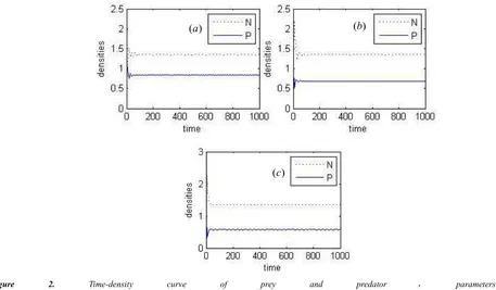
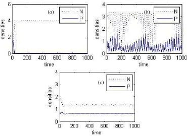
and the system reaches the stable equilibrium state while the positive effect is decreased (see Fig. 2a). The predator, however, tend to extinction if the carrying capacity is increased (see Fig.3a), this phenomenon may be the result of the natural defense of prey. On the contrary, the two species will come into being new ecological phenomena after the prey is harvested. Compared to Fig.1a, the appropriate harvesting will make the periodic system turn to equilibrium (see Fig.1). Fig.1b shows that the fluctuation period does not change, and the frequency of fluctuation is decreased while prey is harvested slightly. The fluctuation period becomes bigger (see
Fig. 1c) and the system turn to equilibrium (Fig. 1d) when the harvesting effort is increased suitably. Fig.2 (harvesting of prey population in the stable system) describes that the system with harvesting is much easier to tend to stable equilibrium than it without harvesting. Fig.3 depicts that, for the case of the prey at its carrying capacity and the predator extinction, the system will occur the situation of Fig.1 when the prey population is harvested. Summary, this study argues further that the appropriate harvesting effort can enhance the stability of the system. The excessive harvesting can lead to the extinction of species.
Figure 1. Time-density curve of prey and predator , parameters are:
0
1.0; 1.0; 5.0; 0.5; 0.2; 2.8; 0.75;
a= b= c= d= L= r= α = i=5.2;K=3;q=0.5; m=2.5; Harvesting effort:( )a E=0; ( )b E=0.5; ( )c E=1.0; ( )d E=1.5.
Figure 2. Time-density curve of prey and predator , parameters are:
0 1.0; 1.0; 5.0; 0.5; 0.2; 2.8; 0.0075;
a= b= c= d= L= r= α = i=5.2;K=3;q=0.5;m=2.5; Harvesting effort:( )a E=0; ( )b E=0.2; ( )c E=0.5
( )a ( )b
( )c ( )d
( )a ( )b
Figure 3. Time-density curve of prey and predator,parameters are:
0 1.0; 1.0; 5.0; 0.5; 0.2; 2.8; 0.75;
a= b= c= d= L= r= α = i=5.2;K=4;q=0.5;m=2.5; Harvesting
effort: ( )a E=0; ( )b E=1; ( )c E=50.
4. Analysis of Bio-Economic Equilibrium
Bio-economic equilibrium implies the ecologic equilibrium and economical equilibrium, that is, xt+1=xt andyt+1=yt
are ecological equilibrium, and the economic equilibrium is defined as economic rent disappear completely.
If constantp is unit price of prey populations that have been harvested. c is the cost of harvest. At timet , the economic rent (net income) can be expressed as follows:
( pqN c E)
dE LN
π= −
+ .
Bio-economic equilibrium is satisfied the following conditions:
maxπ=[pqN (dE+LN)−c E] ;
0 2
(1 N P) c qE 0
r P
K N i N a dE LN
α −
− − − =
+
+ + (6)
2 0
cN
b m
N i+ +N a− = .
In order to the work accords with the realistic situation, we discuss following cases:
Case I: if pqN (dE+LN)<c, the harvest should be stop
because the cost of harvest is much more than the sales prices. Bio-economic equilibrium point is not existence.
Case II: if pqN (dE+LN)>c , the harvest will be on progress because of profit. After calculation from (5), two
bio-economic equilibrium points can be got as follows:
3
N∞=N , 3 2
0
( ( ) ( ) )
( )
r pq cL pd N r K P P
c N i N a αr K ∞ ∞
∞ ∞
− − +
= =
+ + − ,
pq cL
E N
cd
∞= ∞ − ;
4
N∞=N , 4 2
0
( ( ) ( ) )
( )
r pq cL pd N r K P P
c N i N a αr K ∞ ∞
∞ ∞
− − +
= =
+ + − ,
pq cL E N
cd ∞= ∞ − .
Bio-economic equilibrium points exist for pd>cL and close to the positive equilibrium points. If E>E∞ , the harvesting can’t be continued indefinitely because the cost of harvest is more than the incoming. If E<E∞, the cost is less
than the incoming, the harvesting thus can produce positive economic profits.
For explaining clearly the result of the former theoretical analysis, we introduce discrete-time function about the harvesting effort:
1 ( )
t
t t t t
t t
pqN
E E E c E
dE LN
ωπ ω
+ = + = + + − . (7)
Where ϖ is a positive constant which converts savings into capital. Combining with the system (2), we do numerical simulate by Matlab (see Fig.4). In Fig.4, prey density, predator density and harvesting effort are changed corresponding with time t . No matter what the initial values take, all of trajectories will eventually turn to a stable point-—bio-economic equilibrium point—N∞ =1.351,P∞=0.5774,
1.515
E∞ =
( )a ( )b
Figure 4. Phase space trajectories parameters are:a=1.0;b=1.0;c=5.0;d=0.5;L=0.2;r=3.2;α0=0.075; i=5.2;K=3;
0.5; 2.5; 7.6; 0.05
q= m= p= ω= .
5. The Optimal Harvesting Strategy
For the development and utilization of renewable resources, our goal is to maintain ecologic equilibrium and come true the maximum of economic rent. Firstly, the harvesting of prey population has long-term profits if and only if E<E∞
according to the discussion in the section 4. Secondly, the harvesting effort depends on the unit price p of prey populations by equation (7). All of these show that, in order to limit the harvesting effort, the government should control the price of species in order to control the harvesting effort.
The discussions are so far based on the bio-economic equilibrium point. To discuss a dynamically optimal harvesting effort, the present value is expressed as follows:
1
(
)
k
t t
t
t t t
pqN
J
e
c E
dE
LN
δ − ==
−
+
∑
.Where J is the present value. δis the discount rate, and
t
e−δ is the discount factor, Et =E t( )is the harvesting effort in timet . We solve the problem of the optimal harvesting strategy by the discrete Pontryagin maximum principle[24].
The optimal harvesting problem can reduce to the following problem
Performance indicators:
1
max
(
)
k
t t
t
t t t
pqN
e
c E
dE
LN
δ − =−
+
∑
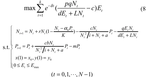
(8)s.t. 0 1 2 1 2 0 0 max (1 )
(1) , (1)
0
t t t t t
t t t t
t t t t
t
t t t t
t t
t
N P cN qE N
N N rN P
K N i N a dE LN
cbN
P P P mP
N i N a
x x y y
E E α + + − = + − − − + + + = + − + + = = ≤ ≤
(t=0,1,⋅⋅⋅,N−1)
WhereNt ,Pt are the state variables, Et is the control
variables.
The corresponding Hamilton function is
0
1(1) 2 1
( ) [ (1 ) ]
t t T t t t t t t t t t t t t
t t t t t t
pqN N P cN qE N
H e c E N rN P N
dE LN K N i N a dE LN
δ λ α
−
+ − +
= − + + − − − −
+ + + +
2( 1) [ 2 1]
T t
t t t t t
t t
cN
P b P mP P
N i N a
λ + +
+ + − −
+ +
1(t 1)
λ + and λ2(t+1)are association state variables.
Due to the function H is linear function of control variableEt, the necessary conditions of optimal problem are
2 2 2
0
1( ) 2 1(1) 2 2 2
2 ( )
[ (1 ) ]
( ) ( ) ( )
t
t t t t t t t
t t
t t t t t t t
H pqdE N P cP a N i qdE
e r
N dE LN K N i N a dE LN
δ α
λ − λ
+
∂ − −
= −∂ = − + − − − + + − +
2
2( 1) 2 2 1( 1)
( )
( )
t t
t t
t t
cPb a N i
N i N a
λ + − λ +
− =
+ + (9)
0
2( ) 1( 1)( 2 ) 2( 1)( 2 ) 2(1)
t t t t
t t t t
t t t t t
H r N cN bcN
m P K N i N a N i N a
α
λ λ + λ + λ +
∂
= − = − − − − =
∂ + + + + (10)
2 2
1( 1)
2 2
[ ] 0
( ) ( )
t t t
t
t t t t t
pqLN qLN
H
e c
E dE LN dE LN
δ λ
−
+
∂ = − − =
∂ + + (11)
Combine equation (9) and (10), we obtain the value of
1(t 1)
λ
+ after calculation. Then the optimal harvesting effort* 1
{ }N t t
E = can be got from equation (11). The harvesting effort
* 1
{ }N t t
E = are satisfied the expression
* * 2
1 *2
( )
[ ]
t t t
t c dE LN e p
qLN δ
λ = − − +
.
According to the optimal balance principle, the corresponding optimal prey and predator population size can be expression as follows: * ( *2 * )
t t t
cbN =m N i+N +a and
* * * * *
* 0 *
*2 * * *
(1 t t) t t t
t t
t t t t
N P cN qE N
rN P
K N i N a dE LN
α
−
− − =
+ + + , respectively.
6. Phase-Plane and Bifurcation Diagram
Analysis
For better understanding the theoretical results, we do the phase-plane and bifurcation diagram by using Matlab programming in this section.
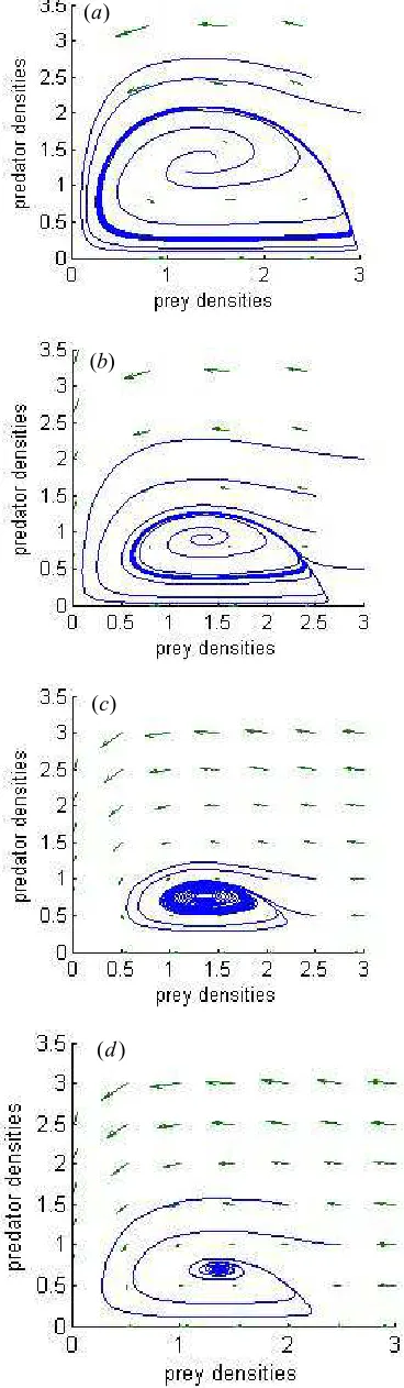
Chao Liu et al. (2009)[23] study a different-algebraic model system which considers a prey-predator system with structure for prey and harvest effort on predator. With the help of Matlab, numerical simulations are provided to substantiate the theoretical result. Here, we have showed numerically the influence of harvesting effort on the local stability of the system (2) in section 4. Next, we provide numerical simulations to the effect of harvest on the equilibrium point (see Fig.5). From Fig.5, we know when the harvesting effort is increased more, the trajectories tend to an unstable point while prey and predator densities are all more than about 2.5. Otherwise, there is a stable limit cycle while prey and predator densities are all less than about 2.5 (see Fig.5d). Secondly, from the stable analysis above, it gains that the limit cycle appears around the positive equilibrium point E3 ( E4 ). In this section, we
Figure 5. Phase-plane diagram of prey and predator. parameters are:
0 1.0; 1.0; 5.0; 0.5; 0.2; 4.5; 0.75;
a= b= c= d= L= r= α = i=5.2;K=3;q=0.5;m=2.5;
Harvesting effort: ( )a E=0; ( )b E=1.0; ( )c E=10; ( )d E=20.
Figure 6. Phase-plane diagram of prey and predator. parameters are:
0 1.0; 1.0; 5.0; 0.5; 0.2; 2.8; 0.75;
a= b= c= d= L= r= α = i=5.2;K=3;q=0.5;m=2.5;
Harvesting effort: ( )a E=0; ( )b E=0.5; ( )c E=1.0; ( )d E=1.5.
( )b
( )c
( )d
( )a
( )a
( )b
( )c
Figure 7. Bifurcation diagram of prey and predator with the initial
conditions x(0)=0.3; (0)y =0.2 . Parameters
are: a=1.0;b=1.0;c=5.0;d=4.5;L=3.2;α0=0.75; i=5.2;K=4;q=1.2;m=2.5; Harvesting effort:( )a E=0; ( )b E=1.0; ( )c E=2.0; ( )d E=3.0.
7. Discussion and Conclusion
It is well known that harvesting has a strong impact on the
dynamic evolution of a population. The biological resources in the prey-predator system are mostly harvested with the aim of achieving.
Economic interest motivates the introduction of harvesting in the prey-predator models. There are many studies, which show that the harvesting effort has effect on the system dynamic, and get the optimal strategy[24-26]. In this paper, we discuss the influence of the harvesting effort on the system with Holling type-IV by using the theoretical analysis and numerical simulations. Firstly, the theoretical analysis shows that the harvesting effort to the prey population influences the stability of the system. Comparing with the system (1), the system (2) has five equilibrium points (see Tab.1) is more than that in the system (1). Our study show that it is the Holling type-IV leads to two positive equilibrium points, and the harvest leads to two boundary equilibrium points. This illustrates that the unreasonable harvest will lead to species easy extinction.
Secondly, for a Long-term perspective of maintaining the ecological equilibrium and the species sustainable development, the theoretical analysis in section 4 provides us a bio-economic way to keep the long-term positive economic interest of harvesting in the system with Holling type-IV. Our study also show that the system achieves different equilibrium (including equilibrium point E0 ) with the parameters changed in the model. Here, we only study the case of harvest around the positive equilibrium point, and it illustrates that the harvest effort is proportional to the price. Thus, the government must control the market price of species.
Thirdly, the study on the optimal harvest strategy in section 5 depicts that there is the optimal harvesting effort
* 1
{ }N t t
E = (corresponding to the optimal population * * 1
{( , )}N
t t t
N P = ).
For example, fur seals and cod, krill system and baleen whales. When we consider competition and the handing time into the system, the results are more close to real world, the bio-economic measures based on the theoretical analysis in this paper can be taken to deal with the impact of the current recession on fishery.
Furthermore, we try to understand the effect of the harvesting effort on the local stability of the model system. By numerical simulation, from this we know that the suitable harvest can make the system easier to get equilibrium. Especially, for the case of the predator extinction while the prey carrying capacity increased, the harvest can make the both of populations coexistence as a result of the prey’s natural defense destroyed. But the excessive harvest leads to the extinction of species and the collapse of the ecosystem. We also understand that, in the system without harvest, there is the limit cycle around the two positive equilibrium points
3
E andE4, respectively, and appears Hopf bifurcation and chaos phenomena. However, in the case of the system with harvest, the constantly harvest not only make the limit cycle become smaller and smaller and finally close to a stable point, but also delay the bifurcation and chaos phenomena appearance.
( )a
( )b
( )c
Acknowledgements
The authors are very grateful to the anonymous referee for his carefully reading and helpful suggestions. This work was supported by grants 1010RJZA127 from the Natural Science Foundation of Gansu and 2007BAD88B07 from the Supportive Plan of China, National Natural Science Foundation of China (No.3126009 and No.31360148).
References
[1] Clark C. W. Mathematical Bio-economics: The Optimal Management of Renewable Resources[M]. 2nd ed., New York: John Wiley and Sons, 1976.
[2] Asep K., Supriatna Hugh P., Possingham. Optimal Harvesting for a Predator-Prey Meta population[J]. Bulletin of Mathematical Biology, 1998, 60(1):49-65.
[3] Lu Zhi-qi, Wei Ping, Pei Li-jun, The Stage-structure Predator-prey Model with a Time Delay and Optimal Harvesting Policy[J]. Journal of Biomathematics, 2003, 18(4):390-394.
[4] T.K. Kav. Conservation of a fishery through optimal taxation: a dynamic reaction model [J]. Communications in Nonlineer Science and Numerical Simulation , 2005, 10:121-131. [5] T.K. Kar, B. Ghosh. Sustainability and economic consequences
of creating marine protected areas in multi-species multi-activity context[J]. Journal of Theoretical Biology, 2013a, 318:81–90.
[6] Wang Shu-zhong, Sun Jia-yi, Li Dong-wei. the Harvest policy for a Class of Discrete Predator-prey System in the Semi-open Resources[J]. Mathematics in practice and theory, 2011, 41(9):186-192.
[7] Reinhard L., Fraanziska H., Matt O. Chapter5-Agent-Based Models and Optimal Control in Biology: A Discrete Approach[J]. Mathematical Concepts and Methods in Modern Biology, 2013, 143-178.
[8] Yousef A., Javad P. Optimal controller design using discrete linear model for a four tank benchmark process[J]. ISA Transactions, 2013, 52(5):644-651.
[9] O. Arino, E. Sanchez, A. Fathallah. State-dependent delay differential equations in population dynamics: Modelling and analysis, in: Fields Institute Communications[J]. American Mathematical Society, Providence, RI, 2001, 29:19-36. [10] S.A. Gourley, Y. Kuang. A stage structured predator-prey
model and its dependence on maturation delay and death rate[J]. Journal of Mathematical Biology, 2004, 49:188-200.
[11] Eduardo L., Pawel P. Global dynamics in a stage-structured discrete-time population model with harvesting[J]. Journal of Theoretical Biology, 2012, 297:148-165.
[12] Raghib A.S., Ziyad A., Mohamed B.H.R.The dynamics of discrete models with delay under the effect of constant yield harvesting[J]. Chaos, Solutions & Fractals, 2013, 54:26-38. [13] Bapan Ghosh, T.K. Kar. Sustainable use of prey species in a
prey-predator system: Jointly determined ecological thresholds and economic trade-offs[J]. Ecological Modelling, 2014, 272: 49-58.
[14] Zijian L., Shouming Z. An impulsive periodic predator-prey system with Holling type III function response and diffusion[J]. Applied Mathematical Modelling, 2012, 36(12):5976-5990. [15] J.H.P. Dawes, M.O. Souza. A derivation of Holling’s type I, II
and III functional responses in predator-prey systems[J]. Journal of Theoretical Biology, 2013, 327: 11-22.
[16] Dawkins R., Krebs J.R. Arms races between and within species[J]. Proceedings of the Royal Society of London, Series B: Biological Sciences, 1979, 202(1161): 489-511.
[17] Qi Jun, Su Zhiyong. Predator-prey syetem with positive effect for prey. Acta Ecologica Sinica, 2011, 31(24):7471-7478. [18] Wensheng Y., Xuepeng L., Zijun B. Permence of Periodic
Holling type-IV predator-prey system with stage structure for prey[J]. Mathematical and Computer Modelling, 2008, 48(5-6):677-684.
[19] Fuyun L., Yuantong X. Hopf bifurcation analysis of a predator-prey system with Holling type IV functional response and time delay[J]. Applied Mathematics and Computation, 2009, 215(4): 1484-1495.
[20] Krishna, S.V., Srinivasu, P.D.N., Kaymakcalan, B. Conservation of an ecosystem through optimal taxation[J]. Bulletin of Mathematical Biology, 1998, 60:569–584. [21] X. Liu, D. Xiao. Complex dynamic behaviors of a discrete-time
predator-prey system[J]. Chaos, Solutions & Fractals, 2007, 32:80-94.
[22] Zheng B.D., Liang L.J., Zhang C.R. Extended Jury criterion[J]. Science China Math., 2010, 53(4):1133-1150.
[23] Chao Liu, Qingling Zhang, Xue Zhang, Xiaodong Duan. Dynamical behavior in a stage-structured differential-algebraic prey-predator model with discrete time delay and harvesting[J]. Journal of Computational and Applied Mathematics, 2009, 231(2): 612-625.
[24] Liu Yan-ping, Wang Wan-xiong, Luo Zhi-xue. Optimal Impulsive Harvesting Policy for a Periodic Gompertz Difference Model[J]. Journal of Quantitative Economics, 2011, 28(2):34-39.
[25] T.K. Kar, B. Ghosh. Sustainability and optimal control of an exploited prey-predator system through provision of alternative food to predator[J]. Biosystems, 2012, 109(2): 220–232. [26] T.K. Kar, B. Ghosh. Impacts of maximum sustainable yield