R E S E A R C H
Open Access
Imputing forest carbon stock estimates from
inventory plots to a nationally continuous
coverage
Barry Tyler Wilson
*, Christopher W Woodall and Douglas M Griffith
Abstract
The U.S. has been providing national-scale estimates of forest carbon (C) stocks and stock change to meet United Nations Framework Convention on Climate Change (UNFCCC) reporting requirements for years. Although these currently are provided as national estimates by pool and year to meet greenhouse gas monitoring requirements, there is growing need to disaggregate these estimates to finer scales to enable strategic forest management and monitoring activities focused on various ecosystem services such as C storage enhancement. Through application of a nearest-neighbor imputation approach, spatially extant estimates of forest C density were developed for the conterminous U.S. using the U.S.’s annual forest inventory. Results suggest that an existing forest inventory plot imputation approach can be readily modified to provide raster maps of C density across a range of pools (e.g., live tree to soil organic carbon) and spatial scales (e.g., sub-county to biome). Comparisons among imputed maps indicate strong regional differences across C pools. The C density of pools closely related to detrital input (e.g., dead wood) is often highest in forests suffering from recent mortality events such as those in the northern Rocky
Mountains (e.g., beetle infestations). In contrast, live tree carbon density is often highest on the highest quality forest sites such as those found in the Pacific Northwest. Validation results suggest strong agreement between the estimates produced from the forest inventory plots and those from the imputed maps, particularly when the C pool is closely associated with the imputation model (e.g., aboveground live biomass and live tree basal area), with weaker agreement for detrital pools (e.g., standing dead trees). Forest inventory imputed plot maps provide an efficient and flexible approach to monitoring diverse C pools at national (e.g., UNFCCC) and regional scales (e.g., Reducing Emissions from Deforestation and Forest Degradation projects) while allowing timely incorporation of empirical data (e.g., annual forest inventory).
Keywords:Forest, Carbon density, Imputation, United States, Forest inventory, Raster maps
Background
Forest ecosystems represent the largest terrestrial carbon (C) sink on earth [1,2], such that the United Nations Framework Convention on Climate Change [3] has recog-nized their management as an effective strategy for offset-ting greenhouse gas (GHG) emissions [4,5]. As part of the Convention, the U.S. has been submitting national reports, the National Greenhouse Gas Inventory (NGHGI), detail-ing emissions and removals of GHGs [3] on an annual basis for many years [6]. In addition to international reporting requirements, GHG budgets are being developed
at sub-national scales including states (e.g., California) and ownerships (e.g, National Forest System climate change scorecard). Forest C stocks in the U.S. are estimated using data from the national forest inventory conducted by the USDA Forest Service, Forest Inventory and Analysis (FIA) program [7]. Broad forest ecosystem components (e.g., aboveground live biomass) have been delineated to generalize C stocks to meet international reporting agree-ments pursuant to refining understanding of global carbon cycling [2,3]. Carbon estimates for the ecosystem compo-nents of forest floor (inclusive of litter, fine woody debris, and humic soil horizons), down dead wood, belowground (BG) biomass, and soil organic matter are calculated by FIA using models based on geographic area, forest type, * Correspondence:[email protected]
USDA Forest Service, Northern Research Station, Forest Inventory and Analysis, St. Paul, MN 55108, USA
and, in some cases, stand age [6,8]. Estimates of above-ground (AG) standing live and dead tree C stocks are based on biomass estimates obtained from inventory tree data [6,9]. Although forest C stock estimates, such as those from FIA, are readily available at national and regional scales [6,7], there is increasing interest in disaggregating these large-scale numerical estimates into maps of continu-ous estimates to enable strategic forest management and monitoring activities geared toward offsetting GHG emis-sions [10] and advancing C dynamics research.
Secondary to the need for spatially continuous forest C maps, numerous constituents (e.g., managers, policy makers, and scientists, forest analysts) require an effi-cient methodology for incorporating annual monitoring information into C maps. Sophisticated approaches to mapping forest C stocks may provide robust estimates of stocks [11], but lack the flexibility to rapidly incorpor-ate annual monitoring information. As numerous forest C pools may change on annual time steps, especially in response to stochastic disturbance events, temporal
accuracy of C maps may often be of equal importance as the need for spatial accuracy. Woodall et al. [12] found that actual standing dead tree C stocks were often sig-nificantly different than those modeled for the same in-ventory plots. Despite the measurement/model error associated with annual forest inventory programs, the temporally dynamic nature of forest ecosystems (e.g., wildfires and wind events) necessitates the incorporation of annual data into map products employed by scientists and stakeholders alike.
Wilson et al. [13] developed a methodology (hereafter referred to as Phenological Gradient Nearest Neighbor, or PGNN, for convenience) for producing maps of tree species occurrence and relative abundance over large areas by utilizing information collected on FIA field plots in conjunction with 250 m pixel resolution raster
data in a k-nearest neighbor (kNN) imputation
frame-work. The PGNN approach builds upon the Gradient Nearest Neighbor (GNN) work of Ohmann and Gregory [14], who integrated nearest-neighbor imputation of FIA
plots with ecological ordination via canonical corres-pondence analysis (CCA). PGNN is best described as a
hybrid of the kNN and GNN approaches, since it also
makes use of CCA but utilizesk nearest neighbors
dur-ing imputation rather than only a sdur-ingle neighbor. An-other distinguishing characteristic is that it utilizes vegetation phenology information derived from multi-temporal satellite imagery, as well as climate, topo-graphic, and ecoregion data compiled at a 250 m pixel resolution. One of the most attractive features of this approach is the efficiency with which a plot identifica-tion map can be produced at the naidentifica-tional scale. In other words, every pixel is assigned a forest inventory plot label as well as the attributes of the labeled plot’s nearest neighbors, as defined by the CCA model. In the case of forest C accounting, every pixel could be assigned C stock estimates in a rapid fashion on an an-nual time-step.
Given the need for C maps at the national scale and the possible application of PGNN, the goal of this study was to apply PGNN for imputing national forest inventory plots
to a spatially continuous raster grid in order to produce
mapped estimates of the conterminous U.S.’s forest C
density with these specific objectives: 1) to produce and in-terpret maps of forest carbon density by individual pools and combinations thereof (total forest ecosystem C density, live tree AG, live tree BG, live understory AG and BG, standing dead tree AG, downed dead wood, forest floor, soil organic carbon, and the pool that has the highest proportion of total forest ecosystem C density); 2) to con-duct validation of the C mapping approach by comparing map-based and field plot-based estimates using a variety of metrics; and 3) to suggest future research directions and applications.
Results
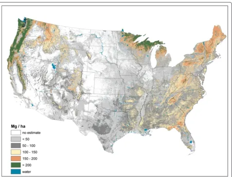
The imputed raster maps of total forest ecosystem C stocks (i.e., sum of all pools) suggest a rather disparate distribu-tion of large total C stocks across the U.S. (Figure 1). While most forested areas of the U.S. have moderate C stock density (< 100 Mg/ha) (e.g., lower elevations of the Rocky Mountains, Central, and Plains states), there are other
areas that have C densities in excess of 200 Mg/ha such as the Pacific Northwest and the upper Great Lakes. As total C stocks are comprised of diverse forest ecosystem compo-nents, examining the distribution of C stock density by component can refine understanding of C density dynam-ics at a national scale.
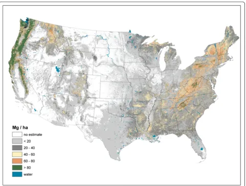
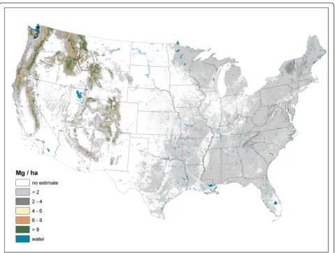
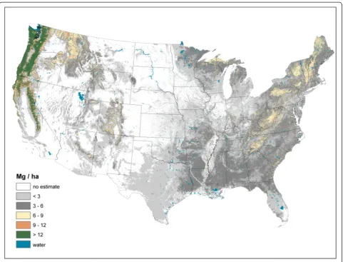
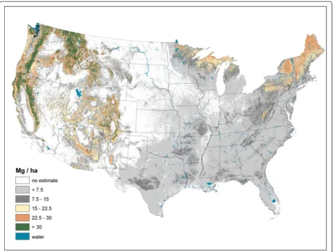
Live AG and BG (Figures 2 and 3) C stock density is highest in the Pacific Northwest, northwest California, northern Rockies, and Appalachian Mountains. The highest live AG C stock density often exceeds 80 Mg/ha. As BG C stocks are modeled as a function of AG C stocks, their spatial distributions are closely aligned. Live understory AG and BG C density follow spatial patterns in allocation similar to live tree distributions, albeit at a much lower density (< 1 Mg/ha) (Figure 4). Standing dead tree C stock densities are highest (> 8 Mg/ha) in the Olympic Mountains, Cascade Range, and North and Central Rocky Mountains (Figure 5). In comparison to the western U.S., eastern standing dead tree C stock density is minimal with only the Adirondacks and iso-lated areas of the Appalachian Mountains having a stock
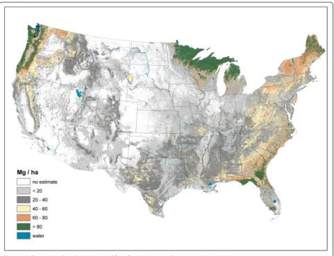
density exceeding 2 Mg/ha. The highest downed dead C stock densities (> 12 Mg/ha) are almost exclusively found in the Pacific Northwest and West Coast/Sierra Nevada (Figure 6). The detrital components of forest floor and SOC have spatial distributions fundamentally different from woody biomass C stock distributions (Figures 7 and 8). The highest C stock densities for forest floor (> 15 Mg/ha) are found in the Pacific Northwest, California, Rocky Mountains, upper penin-sula of MI, and New England. The highest C stock densities for SOC (> 80 Mg/ha) are found in the upper Lake States, Pacific Northwest, northern New England, and coastal areas of the Southeast. In order to better appraise areas subject to varying C stock dy-namics, each pixel was assigned to one of three cat-egories, indicating where it had the largest proportion of its total C stocks apportioned: 1) live biomass (live tree and understory AG and BG), 2) SOC, and 3) dead wood and forest floor (Figure 9). Live biomass is the dominant C stock along the West Coast and Appalachian Mountains. In contrast, SOC is the dominant C stock
along Southeastern coastal areas, New England, Great Lakes, and Great Plain’s forests. The dead wood and for-est floor is dominant in areas of the Rocky Mountains.
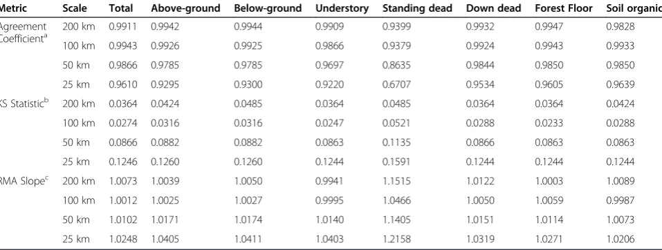
Validation metrics suggest good agreement between map-based and field plot-based estimates of C density across pools and spatial scales (Table 1). The strongest agreement according to all three validation metrics is at the coarsest spatial scale (200 km) with slight reductions in agreement statistics down to the finer spatial scale (50 km). At 25 km, most pools demonstrate a more sub-stantial drop in agreement, albeit most statistics still in-dicate strong agreement (e.g., agreement coefficient above 0.90). The one exception is the standing dead tree C pool which had good agreement at the spatial scale of 100-200 km, but demonstrated a marked decline in agreement down to the finest spatial scale of 25 km (e.g., agreement coefficient = 0.67). The distribution curves and CI maps (Figures 10, 11, 12, 13, 14, 15, 16 and 17) reinforce the fit statistics: there is fairly robust agree-ment between the map-based and field plot-based esti-mates of C density by pool at the finer spatial scale of
50 km (216,500 ha). The differences appear to be distrib-uted in a rather spatially unbiased manner across the conterminous U.S., although there is a tendency for the model to overestimate forest C at the edges of the forested extent. The same phenomenon was present and discussed in the earlier study of species relative abun-dance [13]. This is most likely an effect of the spatial mismatch between pixels and plots, as well as a
mis-match between the “forest” stratum used during
imput-ation and the FIA definition of forest land, that includes a component based on land use not readily detected using remote sensing data.
Discussion
This study demonstrated that a spatially explicit imput-ation approach may be applied to a standard forest in-ventory to efficiently produce continuous maps of forest C stock estimates in a timely manner. Across spatial scales ranging from 25 to 200 km, imputed C stock esti-mates closely matched those derived from the forest
in-ventory data that serve as the basis for the U.S.’s
NGHGI. Thus, the opportunity exists to down-scale a NGHGI to finer scales (e.g., sub-county scale). As vari-ous studies [5,10] have recently highlighted the role that forest management may play in mitigating climate
change, the accurate carbon assessment of “
project-scale”forest management activities is paramount to fore-casting potential mitigation benefits, if any. A project scale C inventory that is consistent with regional and NGHGI’s may allow for robust verification, a desirable at-tribute of forest C projects [15]. In addition, consistency in monitoring forest C across spatial scales may be inte-gral to fully understanding the dynamics of forest C from stands to ecosystems [16]. Beyond the spatial scale, such imputed maps may be rapidly updated annually to in-corporate recent disturbance information. It is expected that large scale disturbance events may increasingly affect forest C stocks in the face of climate change [17]. Disturbance events may occur on annual time steps such that forests become net emitters of C [18] over a relatively short period of time. Recent wildfires and in-sect outbreaks [19] in western North America have
highlighted the need to provide temporally continuous monitoring of forest C stocks. Whether the PGNN ap-proach or alternative is used, spatially explicit imput-ation approaches enable the use of annual forest inventories to inform real-time and real-world C man-agement situations.
Although an imputed forest C map may provide a reasonable down-scaling of a NGHGI, the situation
remains that most NGHGI’s have high variability at
forest analysts will need to develop and apply imput-ation models within the same time frame. Finally, an important component of the PGNN approach used in this study is that the live tree attribute of basal area was a central dependent variable [13]. The imputed maps of standing dead tree C density had the poorest agreement with the empirical inventory present in the NGHGI. It has already been demonstrated in the
U.S.’s NGHGI that detrital C models based on live
tree attributes may substantially over/under-estimate actual C stocks at finer scales (e.g., plot-level) [12]. This may likewise occur with spatial imputation models and it is suggested that future research explore alterna-tive imputation models for the non-living C stocks in forest ecosystems. There was reasonable agreement between the imputed estimates of SOC and the forest floor C densities compared to the NGHGI because the NGHGI currently uses models based partially on live tree attributes to estimate these stocks [6]. How-ever, a comparison between the first empirical inven-tory of forest floor C stocks across the U.S. [21] and
the map in this study (Figure 7) highlights the reduced uncertainty that could be realized by both adopting em-pirical measurements of C pools within a NGHGI and adapting imputation models to fit those unique ecosys-tem components.
Can imputed forest C maps inform our knowledge regarding the dynamics and attributes of C across the U.S.? Perhaps the dynamics of forest C is best illustrated by Figure 9. It is obvious that the predominant forest C pool varies by ecosystem across the U.S.. While at high latitudes or in coastal/wetland areas it may be the SOC and forest floor pools that require the most attention when it comes to management and monitoring, it can be the AG biomass (whether dead or alive) that should be a focal point in most other areas. Most telling was the dominance of detrital forest C pools in most areas of the Intermountain West. The value of imputed forest C maps may be beyond monitoring C monitoring efforts at scales ranging from national to sub-county, rather it may be in identifying emerging research areas and
eco-logical “hotspots” [21] such as areas where forest C
stocks may be responding to climate change events or how detrital and soil organic C stocks may be related.
Conclusions
Down-scaling forest NGHGI’s to finer scales (i.e. project level) is needed to provide project verification that is re-gionally consistent while at the same time refining the science of forest C monitoring. A map-based imputation approach, such as the PGNN technique applied in this study, affords an efficient and timely method for produ-cing spatially continuous maps of diverse forest C pools that are consistent with a NGHGI. The uncertainty asso-ciated with each imputed pixel is dependent on not only the imputation model, but also on the models that underlie the NGHGI. We suggest that further research in both modeling areas be undertaken to refine forest C maps in the future. Until such refinements occur, the maps produced in this study can only provide rough guidance for forest C projects while highlighting the re-gional differences in various C pools and their associated dynamics that in turn may guide future research.
Methods Data
subplot center is established where only live trees with a dbh between 2.5 and 12.7 cm are inventoried.
The field data for this study were taken entirely from the FIA database [8] using the most recent annual col-lection (what FIA refers to as an “evaluation”) of forest inventory plots available at the time of the study for the conterminous 48 states (N.B., annual plots from western Oklahoma, New Mexico, and Wyoming were not avail-able at the time of this study). The data collection period for the annual inventories conducted in most of the states used in this study was initiated since 2000 and ran through 2009, with a full cycle of plots being collected over a 5-year period in the East (roughly 2005-2009) and a 10-year period in the West (roughly 2000-2009). The collection of annual plots used for each state in this
study contained all plots associated with that “
evalu-ation” from the FIA database. This includes
non-forested plots and, by definition, only the data collected from the most recent observation of each plot. Sample intensities vary by state, since some have not yet com-pleted data collection for a full cycle of plots, while
others have chosen to intensify their sampling intensity by 2-3 times the base intensity. FIA field data, with ap-proximate plot locations, are freely available for down-load from the program’s website [25].
These field data were used in conjunction with data extracted at each plot location from a 250 m pixel reso-lution raster stack. This predictor dataset included vege-tation phenology information derived from a time series of vegetation indices based on MODIS satellite imagery (2002-2008), mean monthly climate characteristics from the Daymet climatological model of interpolated climate station observations (1980-1997) [26], topographic metrics from the Elevation Derivatives for National Applications digital elevation model, and Omernik’s Level III ecoregions (or ecological zones) [27]. For a more complete description of these datasets and how they were used in the study, see Wilson et al. [13].
Plot-level carbon estimates
Table 1 Validation metrics by scale and forest C stock
Metric Scale Total Above-ground Below-ground Understory Standing dead Down dead Forest Floor Soil organic
Agreement Coefficienta
200 km 0.9911 0.9942 0.9944 0.9909 0.9399 0.9932 0.9947 0.9828
100 km 0.9943 0.9926 0.9925 0.9866 0.9379 0.9924 0.9943 0.9933
50 km 0.9866 0.9785 0.9785 0.9697 0.8635 0.9844 0.9850 0.9850
25 km 0.9610 0.9295 0.9300 0.9220 0.6707 0.9534 0.9605 0.9639
KS Statisticb 200 km 0.0364 0.0424 0.0485 0.0364 0.0485 0.0364 0.0364 0.0424
100 km 0.0274 0.0316 0.0316 0.0247 0.0521 0.0288 0.0233 0.0288
50 km 0.0866 0.0882 0.0882 0.0863 0.1135 0.0866 0.0863 0.0863
25 km 0.1246 0.1260 0.1260 0.1244 0.1591 0.1244 0.1244 0.1244
RMA Slopec 200 km 1.0073 1.0039 1.0050 0.9941 1.1515 1.0122 1.0003 1.0089
100 km 1.0012 1.0025 1.0027 0.9995 1.0466 1.0050 1.0059 0.9987
50 km 1.0102 1.0171 1.0174 1.0140 1.1405 1.0151 1.0114 1.0073
25 km 1.0248 1.0405 1.0411 1.0403 1.2158 1.0319 1.0271 1.0206
a
Agreement Coefficient (larger values indicate better agreement, min = 0, max = 1).
b
Kolmogorov–Smirnov Statistic (smaller values indicate better agreement, min = 0, max = unbounded).
c
Reduced Major Axis Slope (values closer to 1 indicate better agreement, min, max = unbounded).
with a series of individual tree/site models. Both standing live and dead tree AG C stocks are estimated using the Component Ratio Method (CRM) [9]. Briefly, the CRM facilitates calculation of tree compo-nent biomass (e.g., tops and limbs) as a proportion of the bole biomass (determined through field measured species, diameter, and often height measurements) based on component proportions from Jenkins et al. [28]. Structural deductions (e.g., loss of limbs) and wood density reductions [29] are applied to standing dead trees to account for their inherent loss of wood density and tree components through decay processes [12]. The live BG C stocks are a modeled function of the AG live tree C stocks. Understory (both AG and BG) are modeled as a proportion of the live tree AG and BG stock. The remaining forest C stocks (i.e.
forest floor, downed dead wood, and SOC) are mod-eled as a function of a plot’s forest type, stand age, and ecoregion . While a series of empirical measure-ments (e.g., tree diameter and species composition) are independent variables employed by a series of models (i.e., live tree volume models to soil organic carbon models) to determine plot-level C stocks by pool, these resulting estimates are used as the empir-ical basis for imputation in this study. As the meas-urement/model details vary by individual pool, the NGHGI documentation should be referenced for spe-cific model variables and coefficients [6].
Phenological gradient nearest neighbor technique
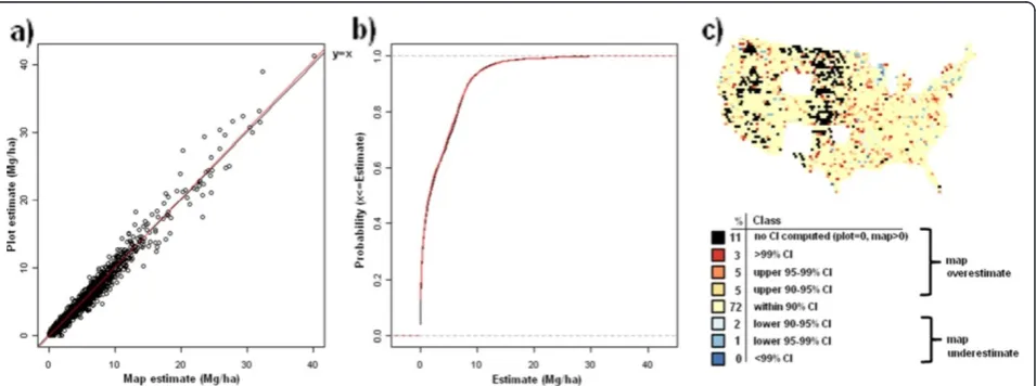
To briefly summarize the methodology described in Wilson et al. [13], CCA models were developed, based on a 1/8th Figure 10Scatterplot, (a), cumulative distribution, (b), and map of confidence intervals of differences (c), between map-based and plot-based estimates of live tree aboveground carbon.Results are based on C density at the spatial scale of 50 km (216,500 ha hexagons).
subsample of the plots, that related the multivariate re-sponse variable measured on the field plots (live tree basal area by species) with the associated 21 predictor variables extracted from the raster stack at each plot lo-cation. For this study, two separate CCA models were constructed: one each for the eastern and western con-terminous United States, using only the plots and pixels found within the respective states and with the central states from North Dakota to Texas being included in each model. The resultant predictor variable loadings (coefficients) were used to transform the predictor vari-ables into a featurespace of “canonical variates” that maximized the inertia in the response data that could be explained by the predictor data. This featurespace was then used to measure proximity between pixels and plots
(more precisely, the pixels containing plots), and thereby to assign a plot label to each pixel in the study area. In an effort to predict a value for each pixel while minimiz-ing the root mean squared prediction error, a small
number of k nearest neighboring plots were used to
im-pute a weighted mean value to each label plot, with the weight assigned to each neighboring plot based on its proximity to the label plot as measured in the feature-space of canonical variates. As in [13], a value of k= 7 and an inverse distance weighting exponent of 1.75 were used to produce the maps in this study. Furthermore, to account for the mismatch in spatial resolution between plots and pixels, a finer spatial resolution dataset of esti-mated tree canopy (i.e., 30 m pixel resolution National Land Cover Database tree canopy cover) was used to Figure 12Scatterplot, (a), cumulative distribution, (b), and map of confidence intervals of differences (c), between map-based and plot-based estimates of downed dead tree carbon.Results are based on C density at the spatial scale of 50 km (216,500 ha hexagons).
stratify the plots into“forest” (> = 25% tree canopy cover) and “non-forest” (< 25% tree canopy cover) strata during the imputation step. Finally, the predicted value for each pixel was calculated as the weighted mean of the imputed values assigned to the corresponding label plot, based independently on “forest” and “non-forest” plots, and the relative proportion of each of these strata present within the pixel.
For the purposes of the current study, all of the model outputs from the earlier study [13] were used: the plot identification (label) raster map, list of neighboring“forest” and“non-forest”plots, plot weights, and strata weights by pixel. These components were used in an analogous fash-ion to compute estimates of forest C stocks for each pixel using the associated plot-level measured or modeled
values, restricting thekplots used for each estimate to the 2nd through 8th nearest neighboring plots.
Map validation
Validation metrics used in this study were similar to those employed by Wilson et al. [13] and described in more detail by Riemann et al. [30]. First, map-based and field plot-map-based estimates were compared at 4 spatial scales (for convenience, these are indi-cated as 25, 50, 100, and 200 km) based on their spatial resolution, which is the distance between the centroids of a spatially continuous mesh of hexagons, using three validation metrics: agreement coefficient (AC), Kolmorogov-Smirnov statistic (KS), and the slope of the reduced major axis (RMA) regression Figure 14Scatterplot, (a), cumulative distribution, (b), and map of confidence intervals of differences (c), between map-based and plot-based estimates of standing dead tree aboveground carbon.Results are based on C density at the spatial scale of 50 km (216,500 ha hexagons).
line. The AC statistic [31] is symmetric and standar-dized describing the agreement in both datasets
about a y = x line. A value of “1” indicates perfect
agreement. The KS statistic quantifies the agreement between the distributions of the two datasets in terms of maximum distance between their empirical distribution functions. The KS statistic makes no assumptions about the distribution of the data and is independent of scale changes. The RMA regression line is calculated in a similar way to the ordinary least squares regression line, but with the assumption that there is error in both the x and y axes and is thus symmetrical regardless of ordering of axes. Fi-nally, scatterplots and cumulative distribution func-tions of map-based versus field plot-based estimates
of C density were determined for each C pool at the spatial scale of 50 km (216,500 ha hexagons). For each C pool, a corresponding choropleth map was constructed that depicts where the map-based estimate for each hexagon falls relative to plot-based confidence intervals (CI). These hexagonal choropleth maps indi-cate which CI (i.e., 90%, 95%, 99%, or greater) the map-based estimate falls within and whether or not the map-based estimate is an overestimate (in the upper half of the CI) or an underestimate (in lower half of the CI) relative to the plot-based estimate. Map-based esti-mates falling within narrower confidence intervals (e.g. 90% CI) suggest better agreement with the associated plot-based estimate than those falling within wider confidence intervals (e.g. greater than 99% CI).
Figure 16Scatterplot, (a), cumulative distribution, (b), and map of confidence intervals of differences (c), between map-based and plot-based estimates of understory aboveground and belowground carbon.Results are based on C density at the spatial scale of 50 km (216,500 ha hexagons).
Competing interests
The authors declare that they have no competing interests.
Authors’contributions
BW developed the mapping methodology, constructed the CCA models, conducted the accuracy assessment, and co-wrote the manuscript. CW compiled the plot-level forest carbon density data, provided the background and analysis of the results of the study, and co-wrote the manuscript. DG conducted the imputation of plot-level data to pixels and produced the maps of forest carbon pools for the study. All authors read and approved the final manuscript.
Received: 14 August 2012 Accepted: 9 January 2013 Published: 11 January 2013
References
1. Pacala SW, Hurtt GC, Baker D, Peylin P, Houghton RA, Birdsey RA, Heath L, Sundquist ET, Stallard RF, Ciais P, Moorcroft P, Caspersen JP, Shevliakova E, Moore B, Kohlmaier G, Holland E, Gloor M, Harmon ME, Fan S-M, Sarmiento JL, Goodale CL, Schimel D, Field CB:Consistent land- and atmosphere-based U.S. carbon sink estimates.Science2001,292:2316–2320. 2. Pan Y, Birdsey RA, Fang J, Houghton R, Kauppi PE, Kurz WA, Phillips OL,
Shvidenko A, Lewis SL, Canadell JG, Ciais P, Jackson RB, Pacala S, McGuire AD, Piao S, Rautiainen A, Sitch S, Hayes D:A large and persistent carbon sink in the world’s forests.Science2011,333:988–993.
3. UNFCCC (United Nations framework convention on climate change). http://unfccc.int.
4. Malmsheimer RW, Heffernan P, Brink S, Crandall D, Deneke F, Galik C, Gee E, Helms JA, McClure N, Mortimer M, Ruddell S, Smith M, Stewart J:Forest management solutions for mitigating climate change in the United States.J Forestry2008,106:115–171.
5. Ryan MG, Harmon ME, Birdsey RA, Giardina CP, Heath LS, Houghton RA, Jackson RB, McKinley DC, Morrison JF, Murray BC, Pataki DE, Skog KE:A synthesis of the science on forests and carbon for US forests.Issues Ecol 2010,13:1–16.
6. U.S. Environmental Protection Agency:Inventory of U.S. greenhouse gas emissions and sinks: 1990-2009. Chapter 7. Land use, land-use change, and forestry. Annex 3.12. Methodology for estimating net carbon stock changes in forest land remaining forest lands. 430-R-11-005. Washington, DC: U.S. Environmental Protection Agency; 2011.
7. Heath LS, Smith J, Skog K, Nowak D, Woodall CW:Managed forest carbon stock and stock-change estimates for the U.S. greenhouse gas inventory, 1990–2008.J Forestry2011,109:167–173.
8. Woudenberg SW, Conkling BL, O’Connell BM, LaPoint EB, Turner JA, Waddell KL:The forest inventory and analysis database: database description and user’s manual version 4.0 For phase 2. Gen. Tech. Rep. RMRS-GTR- 245. Fort Collins, CO: U.S. Department of Agriculture, Forest Service, Rocky Mountain Research Station; 2010.
9. Woodall CW, Heath LS, Domke GM, Nichols M, Oswalt C:Methods and equations for estimating aboveground volume, biomass, and carbon for forest trees in the U.S. forest inventory, 2010. Gen. Tech. Rep. NRS-88. Newtown Square, PA: U.S. Department of Agriculture, Forest Service, Northern Research Station; 2011.
10. Malmsheimer RW, Bowyer JL, Fried JS, Gee E, Izlar R, Reid RA, Munn IA, Oneil E, Stewart WC:Managing forests because carbon matters: integrating energy, products, and land management policy.J Forestry 2011,109:S7–S50.
11. Zhu Z (Ed):A method for assessing carbon stocks, carbon sequestration, and greenhouse gas fluxes in ecosystems of the United States under present conditions and future scenarios. Scientific investigations report 2010-5233. Reston, VA: U.S. Geological Survey; 2010.
12. Woodall CW, Domke GM, MacFarlane DW, Oswalt CM:Comparing field-and model-based stfield-anding dead tree carbon stock estimates across forests of the United States.Forestry2012,85:125–133.
13. Wilson BT, Lister AJ, Riemann RI:A nearest-neighbor imputation approach to mapping tree species over large areas using forest inventory plots and moderate resolution raster data.Forest Ecol Manage2012,271:182–198. 14. Ohmann JL, Gregory MJ:Predictive mapping of forest composition and
structure with direct gradient analysis and nearest-neighbor imputation in coastal Oregon, U.S.A.Can J Forest Res2002,32:725–741.
15. Brown S:Measuring, monitoring, and verification of carbon benefits for forest-based projects.Philos Trans R Soc2002,360:1669–1683. 16. Harmon ME:Carbon sequestration in forests: addressing the scale
question.J Forestry2001,99:24–29.
17. Running SW:Ecosystem disturbance, carbon, and climate.Science2008, 321:652–653.
18. Kurz WA, Dymond CC, Stenson G, Rampley GJ, Carroll AL, Ebata T, Safranyik L:Mountain pine beetle and forest carbon feedback to climate change. Nature2008,452:987–990.
19. Hicke JA, Allen CD, Desai AR, Dietze MC, Hall RJ, Hogg EH, Kashian DM, Moore D, Raffa KF, Sturrock RN, Vogelmann J:Effects of biotic disturbances on forest carbon cycling in the United States and Canada.Global Change Biol2012,18:7–34.
20. Westfall JA, Woodall CW, Hatfield MA:A statistical power analysis of woody carbon flux from forest inventory data.Climatic Change. DOI:10.1007/s10584-012-0686-z. In Press.
21. Woodall CW, Perry CH, Westfall JA:An empirical assessment of forest floor carbon stock components across the United States.Forest Ecol Manage 2012,269:1–9.
22. Smith WB, Miles PD, Perry CH, Pugh SA:Forest resources of the United States, 2007. Gen. Tech. Rep. WO-78. Washington, DC: U.S. Department of Agriculture, Forest Service, Washington Office; 2009.
23. Bechtold WA, Patterson PL (Eds):The enhanced forest inventory and analysis program - national sampling design and estimation procedures. Gen. Tech. Rep. SRS-80. Asheville, NC: U.S. Department of Agriculture, Forest Service, Southern Research Station; 2005.
24. U.S. Department of Agriculture, Forest Service:Forest Inventory and Analysis national core field guide, Volume I: Field data collection procedures for phase 2 plots, version 5.1. Washington, DC: U.S. Department of Agriculture, Forest Service; 2011. http://www.fia.fs.fed.us/library.
25. U.S. Department of agriculture, forest service, forest inventory and analysis DataMart, FIADB version 5.1. http://apps.fs.fed.us/fiadb-downloads/datamart.html.
26. Thornton PE, Running SW, White MA:Generating surfaces of daily meteorological variables over large regions of complex terrain. J Hydrology1997,190:214–251.
27. Omernik JM:Ecoregions of the conterminous United States. Map (scale 1:7500,000).Annals Assoc Am Geographers1987,77:118–125.
28. Jenkins JC, Chojnacky DC, Heath LS, Birdsey RA:National scale biomass estimators for United States tree species.Forest Sci2003,49:12–35. 29. Domke GM, Woodall CW, Smith JE:Accounting for density reduction and
structural loss in standing dead trees: Implications for forest biomass and carbon stock estimates in the United States.Carbon Bal Manage 2011,6:14.
30. Riemann R, Wilson BT, Lister A, Parks S:An effective assessment protocol for continuous geospatial datasets of forest characteristics using USFS Forest Inventory and Analysis (FIA) data.Remote Sensing Environ2010, 114:2337–2352.
31. Ji L, Gallo K:An agreement coefficient for image comparison. Photogrammetric Eng Remote Sensing2006,72:823–833.
doi:10.1186/1750-0680-8-1
Cite this article as:Wilsonet al.:Imputing forest carbon stock estimates from inventory plots to a nationally continuous coverage.Carbon Balance and Management20138:1.
Submit your next manuscript to BioMed Central and take full advantage of:
• Convenient online submission
• Thorough peer review
• No space constraints or color figure charges
• Immediate publication on acceptance
• Inclusion in PubMed, CAS, Scopus and Google Scholar
• Research which is freely available for redistribution