A high-throughput amplicon-based method for estimating outcrossing rates

METHODOLOGY

A high-throughput amplicon-based method

for estimating outcrossing rates

Friederike Jantzen

_{, Natalia Wozniak}

_{, Christian Kappel}

_{, Adrien Sicard}

_{and Michael Lenhard}

Abstract

Background: The outcrossing rate is a key determinant of the population-genetic structure of species and their long-term evolutionary trajectories. However, determining the outcrossing rate using current methods based on PCR-genotyping individual offspring of focal plants for multiple polymorphic markers is laborious and time-consuming.

Results: We have developed an amplicon-based, high-throughput enabled method for estimating the outcrossing rate and have applied this to an example of scented versus non-scented Capsella (Shepherd’s Purse) genotypes. Our results show that the method is able to robustly capture differences in outcrossing rates. They also highlight potential biases in the estimates resulting from differential haplotype sharing of the focal plants with the pollen-donor popula-tion at individual amplicons.

Conclusions: This novel method for estimating outcrossing rates will allow determining this key population-genetic parameter with high-throughput across many genotypes in a population, enabling studies into the genetic determi-nants of successful pollinator attraction and outcrossing.

Keywords: Outcrossing, Mixed mating, Outcrossing rate, Capsella, Amplicon sequencing

© The Author(s) 2019. This article is distributed under the terms of the Creative Commons Attribution 4.0 International License (http://creat iveco mmons .org/licen ses/by/4.0/), which permits unrestricted use, distribution, and reproduction in any medium, provided you give appropriate credit to the original author(s) and the source, provide a link to the Creative Commons license, and indicate if changes were made. The Creative Commons Public Domain Dedication waiver (http://creat iveco mmons .org/ publi cdoma in/zero/1.0/) applies to the data made available in this article, unless otherwise stated.

Background

The rate at which individuals in a population outcross has a major impact on the genetic structure of the popula-tion and its responses to natural selecpopula-tion [1, 2]. While outcrossing maximizes the heterozygosity in a popula-tion, selfing or inbreeding between relatives increases homozygosity. This, in turn, has a number of conse-quences, such as the phenotypic expression of recessive deleterious mutations, also known as inbreeding depres-sion [3], and a reduced rate of effective recombination, as crossing over between homozygous chromosomes does not lead to the formation of genetically recombinant gametes [4]. Over time, such a reduced effective rate of recombination leads to an increased length of haplotype blocks in linkage disequilibrium and of linked selection [4]. In addition, inbreeding reduces the effective popu-lation size, and as a result, the relative importance of genetic drift increases compared to that of selection [5].

The reduced efficacy of purifying selection also increases the risk of fixation of deleterious mutations and influ-ences species extinction rates [6]. Thus, the outcrossing rate is a key determinant of several population-genetic parameters with a major influence on long-term evolu-tionary trajectories of populations [2, 7].

In contrast to animals, where outbreeding enforced by dioecy is seen in the majority of species [8], most flower-ing plants are hermaphrodites [9]. While many plant lin-eages have evolved genetic self-incompatibility and other mechanisms to enforce or promote outbreeding, mixed mating is very common in plants [10]. In mixed-mating species, a fraction of the progeny of a plant is derived from selfing, while the rest is the result of outbreeding. Therefore, estimating the outcrossing rate of plants in a population is an important aspect of studies in plant reproductive systems.

Classically, the outcrossing rate is estimated by geno-typing a large number of progeny individuals from a focal individual for several microsatellite or SNP markers and determining the fraction of genotypes that cannot have been produced by selfing at each marker [11, 12]. From

Open Access

these data, rates of outcrossing and other parameters of the breeding system can then be estimated [13, 14]. While this approach can provide a rich and nuanced picture of the breeding system in a population, it is laborious and thus not readily amenable to be used in a high-through-put manner. Examples for questions that require such a high-throughput approach would be the following. How does the breeding system of a species depend on different environmental conditions? Are rates of outcrossing stable within a population over different years? And how does variation in floral characteristics influence outbreeding rates? Answering this kind of question requires estimat-ing outcrossestimat-ing rates for a large number of focal individu-als, which would be prohibitive when done by genotyping many progeny individuals per focal plant.

Concrete examples for the last of the three mentioned question are studies to determine the relevance of dif-ferent traits presumed to help in pollinator attraction, such as large and showy petals, emission of floral scent, and nectar amount and composition [15]. These traits often undergo large changes, when the breeding system changes from predominant outbreeding to selfing [16]. This transition is generally accompanied by the evolution of the so-called selfing syndrome, comprising a reduc-tion in flower size, especially that of petals, in scent and nectar production and in the ratio of pollen to ovules per flower. One example where the genetic basis of the evolution of the selfing syndrome is being studied is the genus Capsella [17, 18]. This genus contains three diploid species, two of which (C. rubella and C. orientalis) rep-resent independently derived selfers that have diverged from an outbreeding ancestor represented by present-day C. grandiflora between 100,000 and 200,000  years ago and between one and two million years ago, respec-tively [19–21]. Several loci have by now been identified that have contributed to the reduction in petal size and in floral scent in C. rubella compared to C. grandiflora [22– 24]. While this is starting to shed light on the molecular basis and evolutionary history of selfing-syndrome traits, understanding the ecological consequences of changes in presumed pollinator-attraction traits remains a major challenge. That said, several key biological materials have become available as part of the process of gene identifica-tion - such as quasi-isogenic lines (qILs) that only segre-gate for a very small chromosomal segment containing a causal gene, but are essentially isogenic otherwise—that will enable rigorously testing the effect of a given trait change on the interaction with pollinators and herbi-vores, including on the outcrossing rate. However, as outlined above, such studies would greatly benefit from a high-throughput method for estimating outcrossing rates from many individual plants differing in a gene and thus a trait of interest.

Against this background of work on Capsella, we set out to establish and evaluate a high-throughput compat-ible method for estimating and comparing outcrossing rates. This method is based on Illumina sequencing of PCR fragments amplified from pooled progeny individu-als of a plant and estimating the outcrossing rate from the frequency of non-maternal haplotypes.

Methods Reagents

Gibberellic acid 4 + 7 (Duchefa Biochemie) Ethanol (Carl Roth)

Paper bags for bagging plants (HERA)

Bird protection mesh (mesh size 25  mm) (Zill GmbH Co. KG)

Insect protection mesh (mesh size 0.6  mm) (Grow it)

2 ml and 1.5 ml tubes 96 well PCR plates (Sarstedt) Foil/lids to seal plates

384 Well Lightcycler plates (Sarstedt) Adhesive Optical film (Biozym Scientific) Nuclease-free water

Liquid nitrogen

Quiagen DNeasy Plant Mini Kit (Quiagen) AMPure XP beads (Beckmann Coulter) Magnetic stand (Applied Biosystems)

KAPA HiFi Hotstart PCR Kit with dNTPs (Roche) DMSO (Carl Roth)

ROX solution (ThermoFisher Scientific)

SYBR Green I Nucleic acid stain (Sigma-Aldrich) TE buffer (10 mM Tris–HCl, pH 7.5)

QuantiFluor dsDNA System (Promega) Tapestation reagents (Agilent Technologies) Qubit reagents (ThermoFisher Scientific) NextSeq Reagent Kit (Illumina)

Equipment

Mortar and Pistil

Multichannel and single-channel pipettes LightCycler 480 II (or similar) (Roche) Mastercycler nexus (or similar) (Eppendorf)

Speedvac RVC 2-18 (Martin Christ Gefriertrock-nungsanlagen)

NextSeq (Illumina)

Plant material and growth conditions

Two Capsella qILs only differing in about 12 kb around the locus for loss of benzaldehyde emission were com-pared here [23]. A self-compatible Capsella grandiflora

line and qILs segregating for petal size were used as sources to provide pollen for outbreeding [17, 24]. At the beginning of April 2017, seeds were sown on a soil-compost mix and watered with GA-supplemented water (gibberellic acid stock: 16.5  mg in 1  ml ethanol, 1:5000

the oldest fruits started to ripen, individual plants were bagged and allowed to ripen for two more weeks before collection and preparation for DNA extractions. Due to weather conditions and infection with herbivores low numbers of seeds were harvested from each plant. Seeds from all plants with the same genotype within one plot were pooled and cleaned. To be able to define parental haplotypes, we also collected leaf material from the two qILs and subjected it to the same analysis as the seed samples.

DNA extraction from pooled seeds

This method was optimized for extracting DNA from

Capsella seeds. Depending on seed number/size it may need to be adapted. Other extraction methods such as CTAB [25] did not give any results.

1. Approximately 300 seeds were counted into a 2  ml Eppendorf tube to reduce contamination with sand and other dirt. Sterilized water was added and seeds were incubated for 2 days at 4 °C.

2. Transfer seeds into the mortar, remove water by pipetting. Wash 2–3 times with water to remove dirt if necessary.

3. Cool down mortar and pistil with liquid nitrogen and grind samples to a fine powder. Transfer the powder into a new 2 ml tube and add 800 µl Buffer AP1 of Quiagen DNeasy Plant Mini Kit. Store on ice until all samples are ground.

4. Proceed with following steps from Quiagen Kit man-ual, add double amount of buffer AP2 in step 3. For elution in step 12 only 50 µl buffer AE was used. 5. Test extracted DNA in a PCR. If there is no

amplifi-cation and starting material contained a lot of soil or organic matter, try cleaning DNA samples with e.g. AMPure beads.

6. Transfer DNA samples into 96-well plate for further steps.

Design of PCR primers

Next-generation sequencing libraries relying on PCR-based approaches are known to be prone to numer-ous biases linked to amplicon length and GC-content, sequence heterogeneity at primer-annealing sites as well as copy number variation [26–29]. To limit ampli-fication biases, we focused our analysis on low poly-morphic genes present in a single copy within genomes. To this end, we retrieved sequences from single-copy nuclear genes from C. rubella reference genome (https ://phyto zome.jgi.doe.gov/pz/porta l.html) based on [30]. Conserved sites within the Capsella genus were iden-tified by comparing the sequence of 50 C. rubella and

193 C. grandiflora genomes. Primers were designed using Primer 3 plus in order to amplify amplicons of approximately 300 bp and to anneal to their templates at 55  °C. We added 33 and 34 nt sequences comple-mentary to the forward and reverse index primers to each of the gene-specific forward and reverse primers, respectively.

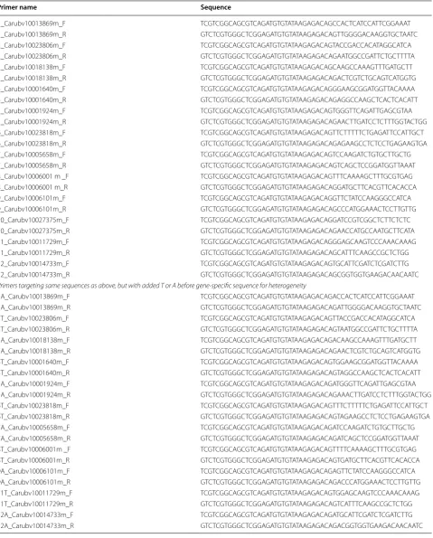
Sequencing quality will also depend on the heterogene-ity of sequences as it is used during the first amplification cycles for cluster identification and phasing/pre-phasing calibration [31]. Low-sequence heterogeneity may impair the distinction between different clusters and consider-ably limit the output of the sequencing run. A common solution to such issues is to co-sequence amplicon librar-ies with a heterogeneous control library (e.g. usually pre-pared from the bacteriophage PhiX genome and mixed at variable proportions, between 15 and 50%) with the drawback that a large number of reads will be lost as they will not correspond to the sequence of the target locus. Here, we introduce sequence heterogeneity by designing an additional primer pair for each target loci contain-ing an additional nucleotide between the gene-specific sequence and those complementary to the indexing primers (Tables 1, 2).

PCR amplification and library generation

The method for PCR amplification and library prepara-tion is based on a recent protocol for amplicon-based microbiome characterization [32]. Further details and troubleshooting information can be found in [32].

This protocol is optimized for low sample DNA con-centrations due to the availability and quality of start-ing material. For best results, minimize PCR cycles and select the samples with the highest concentrations in step 1c. Sample dilution might result in bottlenecking for low abundance alleles as described [32].

1. Primary PCR

a. Create a sample dilution plate.

Table 1 Primers for Primary PCR

Primer name Sequence

1_Carubv10013869m_F TCG TCG GCA GCG TCA GAT GTG TAT AAG AGA CAG CCA CTC ATC CAT TCG GAAAT

1_Carubv10013869m_R GTC TCG TGG GCT CGG AGA TGT GTA TAA GAG ACA GTT GGG GAC AAG GTG CTA ATC

2_Carubv10023806m_F TCG TCG GCA GCG TCA GAT GTG TAT AAG AGA CAG TAC CGA CCA CAT AGG CATCA

2_Carubv10023806m_R GTC TCG TGG GCT CGG AGA TGT GTA TAA GAG ACA GAA TGG CCG ATT CTG CTT TTA

3_Carubv10018138m_F TCG TCG GCA GCG TCA GAT GTG TAT AAG AGA CAG CAA GCC AAA GTT TGA TGCTT

3_Carubv10018138m_R GTC TCG TGG GCT CGG AGA TGT GTA TAA GAG ACA GAC TCG TCT GCA GTC ATG GTG

4_Carubv10001640m_F TCG TCG GCA GCG TCA GAT GTG TAT AAG AGA CAG GGA AGC GGA TGG TTA CAAAA

4_Carubv10001640m_R GTC TCG TGG GCT CGG AGA TGT GTA TAA GAG ACA GAG GCC AAG CTC ACT CAC ATT

5_Carubv10001924m_F TCG TCG GCA GCG TCA GAT GTG TAT AAG AGA CAG TGG GTT CAG ATT GAG CGTAA

5_Carubv10001924m_R GTC TCG TGG GCT CGG AGA TGT GTA TAA GAG ACA GAA CTT GAT CCT CTT TGG TAC TGG

6_Carubv10023818m_F TCG TCG GCA GCG TCA GAT GTG TAT AAG AGA CAG TTC TTT TTC TGA GAT TCC ATT GCT

6_Carubv10023818m_R GTC TCG TGG GCT CGG AGA TGT GTA TAA GAG ACA GAG AAG CCT CTC CTG AGA AGT GA

7_Carubv10005658m_F TCG TCG GCA GCG TCA GAT GTG TAT AAG AGA CAG TCC AAG ATC TGT GCT TGCTG

7_Carubv10005658m_R GTC TCG TGG GCT CGG AGA TGT GTA TAA GAG ACA GTC AGC TCC GGA TGG TTA AAT

8_Carubv10006001 m _F TCG TCG GCA GCG TCA GAT GTG TAT AAG AGA CAG TTT CAA AAG CTT TGC GTGAG

8_Carubv10006001 m_R GTC TCG TGG GCT CGG AGA TGT GTA TAA GAG ACA GGA TGC TTC ACG TTC ACA CCA

9_Carubv10006101m_F TCG TCG GCA GCG TCA GAT GTG TAT AAG AGA CAG GTT CTA TCC AAG GGC CATCA

9_Carubv10006101m_R GTC TCG TGG GCT CGG AGA TGT GTA TAA GAG ACA GCC CAT GGA AAC TCC TTG TTG

10_Carubv10027375m_F TCG TCG GCA GCG TCA GAT GTG TAT AAG AGA CAG GAT CCG TCG GCT CTT CTCTC

10_Carubv10027375m_R GTC TCG TGG GCT CGG AGA TGT GTA TAA GAG ACA GAA CCA TGC CAA TGC TTC ATA

11_Carubv10011729m_F TCG TCG GCA GCG TCA GAT GTG TAT AAG AGA CAG GGA GCA AGT CCC AAA CAAAG

11_Carubv10011729m_R GTC TCG TGG GCT CGG AGA TGT GTA TAA GAG ACA GCA TTT CAA GCC GCT CTGG

12_Carubv10014733m_F TCG TCG GCA GCG TCA GAT GTG TAT AAG AGA CAG TGC ATT CGA TCT CGA TCTTG

12_Carubv10014733m_R GTC TCG TGG GCT CGG AGA TGT GTA TAA GAG ACA GCG GTG GTG AAG ACA ACA ATC

Primers targeting same sequences as above, but with added T or A before gene-specific sequence for heterogeneity

1A_Carubv10013869m_F TCG TCG GCA GCG TCA GAT GTG TAT AAG AGA CAG ACC ACT CAT CCA TTC GGA AAT

1A_Carubv10013869m_R GTC TCG TGG GCT CGG AGA TGT GTA TAA GAG ACA GAT TGG GGA CAA GGT GCT AAT C

2T_Carubv10023806m_F TCG TCG GCA GCG TCA GAT GTG TAT AAG AGA CAG TTA CCG ACC ACA TAG GCA TCA

2T_Carubv10023806m_R GTC TCG TGG GCT CGG AGA TGT GTA TAA GAG ACA GTA ATG GCC GAT TCT GCT TTT A

3A_Carubv10018138m_F TCG TCG GCA GCG TCA GAT GTG TAT AAG AGA CAG ACA AGC CAA AGT TTG ATG CTT

3A_Carubv10018138m_R GTC TCG TGG GCT CGG AGA TGT GTA TAA GAG ACA GAA CTC GTC TGC AGT CAT GGT G

4T_Carubv10001640m_F TCG TCG GCA GCG TCA GAT GTG TAT AAG AGA CAG TGG AAG CGG ATG GTT ACA AAA

4T_Carubv10001640m_R GTC TCG TGG GCT CGG AGA TGT GTA TAA GAG ACA GTA GGC CAA GCT CAC TCA CAT T

5A_Carubv10001924m_F TCG TCG GCA GCG TCA GAT GTG TAT AAG AGA CAG ATG GGT TCA GAT TGA GCG TAA

5A_Carubv10001924m_R GTC TCG TGG GCT CGG AGA TGT GTA TAA GAG ACA GAA ACT TGA TCC TCT TTG GTA CTGG

6T_Carubv10023818m_F TCG TCG GCA GCG TCA GAT GTG TAT AAG AGA CAG TTT CTT TTT CTG AGA TTC CAT TGCT

6T_Carubv10023818m_R GTC TCG TGG GCT CGG AGA TGT GTA TAA GAG ACA GTA GAA GCC TCT CCT GAG AAG TGA

7A_Carubv10005658m_F TCG TCG GCA GCG TCA GAT GTG TAT AAG AGA CAG ATC CAA GAT CTG TGC TTG CTG

7A_Carubv10005658m_R GTC TCG TGG GCT CGG AGA TGT GTA TAA GAG ACA GAT CAG CTC CGG ATG GTT AAA T

8T_Carubv10006001m _F TCG TCG GCA GCG TCA GAT GTG TAT AAG AGA CAG TTT TCA AAA GCT TTG CGT GAG

8T_Carubv10006001m_R GTC TCG TGG GCT CGG AGA TGT GTA TAA GAG ACA GTG ATG CTT CAC GTT CAC ACC A

9A_Carubv10006101m_F TCG TCG GCA GCG TCA GAT GTG TAT AAG AGA CAG AGT TCT ATC CAA GGG CCA TCA

9A_Carubv10006101m_R GTC TCG TGG GCT CGG AGA TGT GTA TAA GAG ACA GAC CCA TGG AAA CTC CTT GTT G

11T_Carubv10011729m_F TCG TCG GCA GCG TCA GAT GTG TAT AAG AGA CAG TGG AGC AAG TCC CAA ACA AAG

11T_Carubv10011729m_R GTC TCG TGG GCT CGG AGA TGT GTA TAA GAG ACA GTC ATT TCA AGC CGC TCTGG

12A_Carubv10014733m_F TCG TCG GCA GCG TCA GAT GTG TAT AAG AGA CAG ATG CAT TCG ATC TCG ATC TTG

For primary PCR, pipet 3 µl of every sample and dilutions into a new 384-well plate which can be used in LightCycler 480 II. Start with the lowest concentration in quadrant 4 (B02) and then pro-ceed with quadrant 3, 2 and 1 to use the same set of tips. Plates can be stored at − 20 °C or used for subsequent primary PCR.

b. Primary PCR

Prior to PCR, test primers individually and pooled for amplification of target genes. Figure 2a shows amplification products for 11 out of 12 primer pairs, in Fig. 2b the pooling strategy was tested for two sets of primer pairs. For the pri-mary PCR, a maximum of six different primer pairs was pooled (including primer pairs with added bases for heterogeneity, so 12 primer pairs overall).

Thaw the Kapa HiFi Hotstart kit reagents and the 384-sample plate if it was stored in the freezer. Vortex and centrifuge all reagents when thawed before using.

Prepare a 2 × KAPA HiFi Hotstart qPCR mas-ter mix with the following components: 1.2  µl 5 × KAPA HiFi Fidelity buffer, 0.18  µl 10  mM dNTPs, 0.3  µl DMSO, 0.12  µl ROX (25  µM),

0.003 µl 1000 × SYBR Green, 0.12 µl KAPA HiFi Hotstart Polymerase, 0.3 µl forward primer pool (10 µM), 0.3 µl reverse primer pool (10 µM) and 0.48 µl nuclease-free water.

Dispense 3 µl of 2 × KAPA HiFi Hotstart qPCR master mix in each reaction well on the 384-well plate containing DNA samples for a final volume of 6 µl.

Cover the plate, mix and spin-down. Start the fol-lowing qPCR protocol on Roche LightCycler 480 II (or similar) after loading the plate: 95  °C for 5 min, then 15 cycles of 98 °C 20s, 55 °C for 15s, 72 °C for 1 min. Cycle number can be between 15 and 30 cycles but optimal results will be achieved by keeping the cycle number low. However, sam-ples amplifying poorly could be amplified using more cycles. Plates can be stored at -20 °C. c. Analysis and choosing the best dilution for

index-ing PCR

The analysis was done manually. For more details on how to conduct it automatically, please refer to [32].

Compare the amplification curves for the differ-ent dilutions of the same DNA sample. Choose a sample concentration which is in the mid-to-late

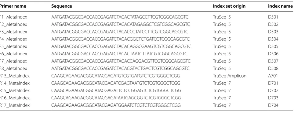
Table 2 Primers for indexing PCR (indexed sequencing primers)

Primer name Sequence Index set origin index name

F1_MetaIndex AAT GAT ACG GCG ACC ACC GAG ATC TAC ACT ATA GCC TTC GTC GGC AGC GTC TruSeq i5 D501

F2_MetaIndex AAT GAT ACG GCG ACC ACC GAG ATC TAC ACA TAG AGG CTC GTC GGC AGC GTC TruSeq i5 D502

F3_MetaIndex AAT GAT ACG GCG ACC ACC GAG ATC TAC ACC CTA TCC TTC GTC GGC AGC GTC TruSeq i5 D503

F4_MetaIndex AAT GAT ACG GCG ACC ACC GAG ATC TAC ACG GCT CTG ATC GTC GGC AGC GTC TruSeq i5 D504

F5_MetaIndex AAT GAT ACG GCG ACC ACC GAG ATC TAC ACA GGC GAA GTC GTC GGC AGC GTC TruSeq i5 D505

F6_MetaIndex AAT GAT ACG GCG ACC ACC GAG ATC TAC ACT AAT CTT ATC GTC GGC AGC GTC TruSeq i5 D506

F7_MetaIndex AAT GAT ACG GCG ACC ACC GAG ATC TAC ACC AGG ACG TTC GTC GGC AGC GTC TruSeq i5 D507

F8_MetaIndex AAT GAT ACG GCG ACC ACC GAG ATC TAC ACG TAC TGA CTC GTC GGC AGC GTC TruSeq i5 D508

R13_MetaIndex CAA GCA GAA GAC GGC ATA CGA GAT GTC GTG ATG TCT CGT GGG CTCGG TruSeq Amplicon A701

R14_MetaIndex CAA GCA GAA GAC GGC ATA CGA GAT CGA GTA ATG TCT CGT GGG CTCGG TruSeq i7 D701

R15_MetaIndex CAA GCA GAA GAC GGC ATA CGA GAT TCT CCG GAG TCT CGT GGG CTCGG TruSeq i7 D702

R16_MetaIndex CAA GCA GAA GAC GGC ATA CGA GAT AAT GAG CGG TCT CGT GGG CTCGG TruSeq i7 D703

R17_MetaIndex CAA GCA GAA GAC GGC ATA CGA GAT GGA ATC TCG TCT CGT GGG CTCGG TruSeq i7 D704

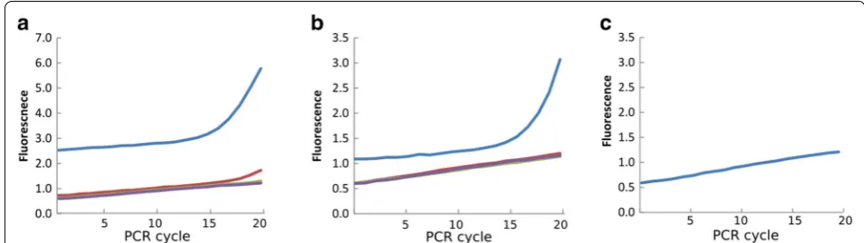
exponential phase at the last amplification cycle of the PCR for further steps. Samples should not have reached a plateau at the final cycle as this means overamplification. Figure 3a, b show two examples of amplification curves, due to low DNA concentrations samples were only in the early-exponential phase but were still used for further steps.

Prepare 96 well plate by distributing 18 µl water in each well. Spin down qPCR plate and trans-fer 2 µl of the appropriate dilution into the new plate to create a 1:10 dilution of the primary PCR. Mix and spin down. (If samples were in mid-to-late exponential phase after the final PCR cycle, transfer 5 µl of 1:10 dilution into a new plate con-taining 45  µl water to generate a 1:100 dilution of primary PCR. Use this instead of 1:10 dilution for further steps). Store at − 20 °C or progress to indexing PCR.

2. Indexing PCR

a. Picking an indexing scheme

Each sample needs to have an individual combi-nation of i5 and i7 indices to make sure no index overlap between pooled samples can occur. Prior to running the PCR an i5 and i7 dual-index-ing scheme needs to be chosen, dependdual-index-ing on how many samples will be pooled together for sequencing. The number of samples is equal to the number of index combinations needed.

See Illumina guide for more information on dual indexing: https ://suppo rt.illum ina.com/conte nt/

dam/illum ina-suppo rt/docum ents/docum entat ion/syste m_docum entat ion/miseq /index ed-seque ncing -overv iew-guide -15057 455-04.pdf

For the design of Illumina adapter sequences see:

https ://suppo rt.illum ina.com/conte nt/dam/illum ina-suppo rt/docum ents/docum entat ion/chemi stry_docum entat ion/exper iment -desig n/illum ina-adapt er-seque nces-10000 00002 694-09.pdf

b. Indexing PCR

Prepare an oligo plate, adapted to your indexing scheme.

Make 10  µM dilutions of your 100  µM primer stocks in a 96 well plate by adding 30 µl 100 µM oligo stock to 270 µl water; forward primers were arranged in columns and reverse primers in rows. For the 5  µM master plate containing 40  µl

primer mix, add 10 µl of the 10 µM forward and reverse primer dilutions into a new plate and add 20  µl water. Mix well and use 2  µl for indexing PCR. See Additional file 1: Table S1 for indexing scheme used in this study. [Please note that of the 38 different index combinations shown in Addi-tional file 1: Table S1, only 12 were used for sam-ples analyzed in this study.]

Thaw the KAPA HiFi Hotstart PCR kit reagents and the primary PCR dilution plate (1:10 or 1:100) if necessary. Mix and spin down reagents. Prepare a 3.33 KAPA HiFi Hotstart Indexing

PCR master mix consisting of these components: 2 µl 5 × KAPA HiFi Fidelity buffer, 0.3 µl 10 mM dNTPs, 0.5 µl DMSO, 0.2 µl KAPA HiFi Hotstart Polymerase. Dispense 3 µl into wells of a 96-well PCR plate. Add 5  µl of diluted primary PCR

product to the corresponding wells in the 96-well PCR plate that contains 3 µl of the indexing PCR master mix. Add 2 µl of 5 µM indexing primers from the prepared oligo plate for indexing. The final reaction volume is 10 µl.

Seal the plate, mix and spin down. Amplify in PCR-machine with the following conditions: 95 °C for 5 min, 10 cycles of 98 °C for 20 s, 55 °C for 15 s, 72 °C for 1 min. Centrifuge the plate to collect the samples after PCR program is com-plete. The plate can be stored at − 20 °C.

3. Normalization and pooling

There are different options for normalization and pooling, depending on available systems and rea-gents. Please check protocol by Gohl et al. for further information [32].

a. QuantiFluor quantification of indexed samples

Calculate DNA concentrations of indexed sam-ples following the manufacturer’s protocol for the QuantiFluor dsDNA system. Use two times 1 µl indexing PCR reaction per sample for quantifica-tion, so 8 µl are left for normalization.

b. Sample normalization

Choose a concentration for normalization. It depends on how concentrated/diluted your sam-ples are. Calculate the amount of water for each sample to be added to a fixed amount of indexing PCR in order to get the desired concentration. For this experiment, 4 µl indexing PCR were used and 5 ng/µl were determined as desired concen-tration. The amount of water to add fluctuated from 0 to 90 µl, depending on sample concentra-tion.

Seal plate, mix and spin down. The plate can be stored at − 20 °C.

c. Pooling and clean-up

Pool identical volumes of all samples for the library. Here, 3.5 µl of each sample normalized to 5 ng/µl were used. Mix and transfer to a 1.5 ml Eppendorf tube. Use Speedvac to collect pool in 20–100  µl. Clean sample pool by using 1 ×

AMPure XP beads (see Appendix 2 of [32]) and elute in 20 µl TE buffer.

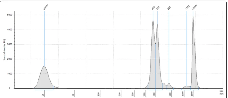
d. Verify quality and size distribution of pooled library

The expected size distribution should be around 500  bp, as primers for primary PCR were designed to keep variable regions between 300 and 400  bp long and approximately 170  bp were added for Illumina Sequencing (including sequences for read 1 and read 2, indices and i5/ i7). Verify size range and distribution by running the library on 2200 TapeStation, following the manufacturer’s protocol.

Determine library concentration by using Qubit 2.0 Fluorometric Quantification and following the manufacturer’s protocol.

Submit the library to your sequencing facility or follow instructions provided by [32].

Amplicon sequencing

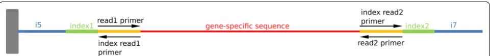
Sequencing can be performed on a NextSeq sequenc-ing platform ussequenc-ing a NextSeq Reagent Kit MidOutput (300 cycles). The library is compatible with the standard sequencing primers, final amplicon structure is shown in Fig. 4.

Sequence analysis and estimation of outcrossing rates

haplotype proportions. Haplotypes with a frequency above 1%, but only present in one single sample were also excluded as they are likely to be a consequence of an early PCR amplification error. Roughly half of the fragments were filtered out that way (see Additional file 2: Table S2). The sums of remaining fragments per sample and ampli-con were then used as a baseline to calculate (1) the pro-portions of parental (P1 or P2) haplotypes per sample and amplicon and (2) the proportions of P1 and P2 haplotypes for the polymorphic amplicon 6_Carubv10023818  m. Data analyses were done using R (https ://www.r-proje ct.org). Illustrations were done using the R/lattice pack-age (http://lmdvr .r-forge .r-proje ct.org).

Results

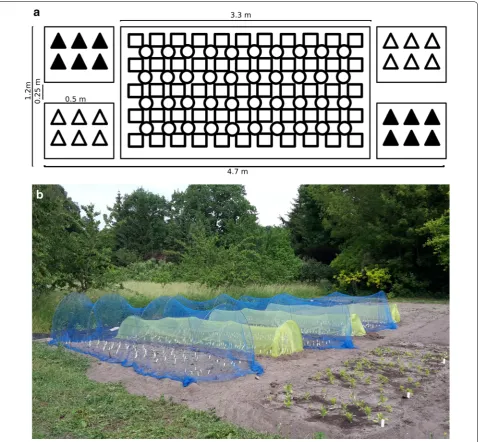
Plants of two Capsella qILs differing in about 12  kb around the CNL1 locus that underlies the loss of benzal-dehyde emission in C. rubella [23] were grown at the field site of the Botanical Garden of the University of Potsdam. The arrangement of the plants is shown in Fig. 1. Each block contained two sets of six plants each of both gen-otypes arranged on opposite sides of a central area with inbred, self-compatible C. grandiflora plants and near-isogenic lines differing for the SAP locus that affects petal size [24]. The plants in this central area served as pollen donors with different background genotypes. Three such blocks were protected from birds and rodents by a bird net, while three such blocks were covered by an insect-proof net.

We designed 12 primer pairs in exons of highly con-served genes that anneal to invariant nucleotide stretches across a large number of C. grandiflora and C. rubella

genotypes. Primers were chosen in exons flanking an intron to maximize the sensitivity for detecting non-maternal genotypes, as intron sequences are generally more variable than exonic sequences. As shown in Fig. 2, 11 out of the 12 primer pairs successfully amplified and two pools of six and five primer pairs were set up to mini-mize the number of required PCR reactions.

Genomic DNA was extracted from approximately 300 pooled seeds from the 12 scented and the 12 non-scented qIL plants per block. A previously described qPCR-based approach [32] was used to determine the optimal tem-plate concentration for the primary PCRs with the two pools of six and five primer pairs described above. Exam-ple results for this test are shown in Fig. 3. In most cases, the undiluted sample was used for further steps.

Barcoding indices were introduced via a second, index-ing PCR, resultindex-ing in final amplification products with the structure shown in Fig. 4. Products from the two primary PCRs (with the six- and five-primer pair pools, respectively) were combined in equimolar ratios after this indexing PCR. An example of a final library pool as determined by Tape Station electrophoresis is shown in Fig. 5.

fragments were retained (Additional file 2: Table S2). We assigned these remaining fragments to either parental or non-parental haplotypes by comparison to the results from the leaf samples of the qILs processed in parallel. Across all amplicons, the frequency of non-parental reads was consistently higher in the samples from plants grown under the bird-protection nets only, i.e. accessible to insects, than from those grown under insect-proof nets (Fig. 6); in fact, in the latter no non-parental haplotypes could be detected for eight of the amplicons in five out of the six samples. In the samples from the bird nets, the fre-quency of non-parental haplotypes reached between 10 and 20% for eight of the amplicons, with very consistent estimates across the individual samples. For three of the amplicons, the frequency of non-parental haplotypes was below 10% in the bird-net samples, again with consist-ent estimates across the individual samples. We ascribe

this difference between the two groups of amplicons to haplotype sharing with the other plants in the blocks that served as pollen donors for the outbred seeds, with at least some of the genotypes sharing the parental haplo-types with our lines at the three amplicons in question, thus rendering many outcrossing events undetectable. Given the simple genetic structure of the pollen-donor populations (two NILs and one inbred C. grandiflora-like line), the extent of haplotype sharing is most likely the same for the eight amplicons with the higher estimates. Thus, the average values across these eight amplicons (Fig. 7) represent the basis of our best estimate of the outcrossing rate in our samples; in particular, given the diploid nature of the plants, the frequency of non-paren-tal haplotypes has to be multiplied by two to obtain an estimate for the fraction of outcrossed seeds, i.e. the out-crossing rate. These values are shown in Table 3. While Fig. 6 Non-parental haplotype frequencies across the amplicons. Non-parental haplotype frequencies are plotted across the 11 amplicons.

these values were higher for the samples from plants with the C. grandiflora CNL1 haplotype than with the C. rubella haplotype for two of the replicates under the bird net, this was reversed in the third replicate. Thus, overall

there was no consistent difference in the estimated out-crossing rate between benzaldehyde-emitting and non-emitting plants in this one trial.

In summary, the strong and consistent difference in apparent outcrossing frequencies between samples under the two types of nets strongly supports the validity of our analysis method and indicates a surprisingly high rate of insect-mediated outcrossing in these self-compatible

Capsella genotypes.

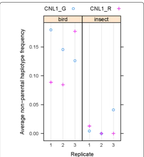
We also found that the two parental lines differed at one of the amplicons (number 6, locus Carubv10023818 m), indicating that their genomic background was not fully isogenic. In principle, this difference could allow esti-mating outcrossing between the two parental lines. When considering only the two parental haplotypes, the plants with the C. rubella haplotype in the CNL1 region appeared to have received more pollen with the alterna-tive haplotype at amplicon 6 (i.e. from the plants with the C. grandiflora haplotype at CNL1) than vice versa under the bird nets (Fig. 8). While this difference could suggest asymmetric pollen flow between the two lines, it could also be due to differential haplotype sharing with the other plants in the plots, in particular, if the plants carrying the C. grandiflora CNL1 haplotype shared their amplicon-6 haplotype with more of the other pollen-donor plants. To circumvent this issue of differential hap-lotype-sharing, only haplotypes found in neither of the two parental lines were counted for the analysis at ampli-con 6 shown in Fig. 6.

Discussion

In this study, we have described a method for estimat-ing outcrossestimat-ing rates that lends itself to the analysis of many samples with high throughput and have validated the method using a common-garden experiment com-paring the outcrossing rate between open-pollinated and insect-excluded plants. Our results clearly show that the method successfully detects insect-mediated ing events and provides consistent estimates of outcross-ing rates across replicated samples. While the analysis approach presented assumes that the maternal genotypes at the tested amplicons are known, the method can eas-ily be adapted to the case when these are not, by prepar-ing a parallel set of amplicon-sequencprepar-ing libraries from genomic DNA of the mother plants to be analyzed.

The described method offers a major advantage regard-ing the time and effort required to estimate the out-crossing rate for many samples. For example, obtaining the estimates for the twelve samples in our study using the classical method would have required running more than 10,000 individual PCR reactions and analyzing the products by electrophoresis (assuming 100 progeny seeds were genotyped per sample). At the same time, the Fig. 7 Mean non-parental haplotype frequencies across the

high-scoring eight amplicons. Mean values across the amplicons 1, 3, 4, 5, 8, 9, 11, 12 are plotted for the twelve samples. Statistical analysis by paired t test between the two genotypes under bird nets or between the two genotypes under insect nets did not detect any significant difference (p > 0.05 in both cases). By contrast, the difference between all samples under bird nets versus all samples under insect nets was highly significant at p < 0.001 based on a Welch two-sample t-test

Table 3 Estimated outcrossing rates (based on Fig. 7)

Genotype Net Replicate Outcrossing rate

CNL1_G Bird 1 0.36

CNL1_G Bird 2 0.29

CNL1_G Bird 3 0.25

CNL1_R Bird 1 0.18

CNL1_R Bird 2 0.16

CNL1_R Bird 3 0.35

CNL1_G Insect 1 0.01

CNL1_G Insect 2 0

CNL1_G Insect 3 0.08

CNL1_R Insect 1 0.03

CNL1_R Insect 2 0

degree of pooling libraries derived from different samples for the sequencing run could easily be increased, enabling the analysis of more samples with very little extra effort. For example, when demanding on average a 10,000-fold coverage for each of ten amplicons per sample, hundreds of samples could be analysed in parallel using a single NextSeq mid-output run. In principle, this would allow very fine-scale descriptions of how the outcrossing rate differs across a population to determine the effect of environmental influences or trait variation.

Compared with the single progeny-based approach these advantages concerning throughput come at a cost

regarding the up-front investment in primer design and the precision of the estimates of outcrossing rates. As for primer design, one obvious technical source of error is differential amplification efficiency of different hap-lotypes due to mismatches in the primer-binding sites. For individual-based measurements, only very large dif-ferences in amplification efficiencies will cause an error, causing, for example, certain heterozygotes to be called as homozygotes for the more efficiently amplifying allele. By contrast, even slight amplification biases for different haplotypes can cause substantial error in the estimated outcrossing rates using the method described here. To circumvent this issue, some up-front sequenc-ing of the haplotypes in the population in question may be necessary to identify highly conserved primer-bind-ing sites. Followprimer-bind-ing the strategy taken here, a cost-effec-tive method for doing so would be to sequence PCR amplification products from highly conserved genes containing one or more introns from many pooled indi-viduals in the population. Analysis of these sequences should allow identifying invariant primer-binding sites flanking suitably polymorphic regions or adapting the primer design by incorporating polymorphic bases into the primers, if no fully invariant regions can be found. The strategy for primer design is outlined in Additional file 4: Figure S1.

As for the precision of the estimates, the present method will necessarily underestimate the true out-crossing rates, and it will do so more strongly than the individual-based method in most cases. Concerning each single amplicon, the true outcrossing rate will be underestimated by the combined frequency of the one or two maternal alleles in the pollen population, as any outcrossing event involving a pollen-carrying one of the maternal alleles will be undetectable when considering a single amplicon. The individual-based method is bet-ter able to deal with this complication than the pool-based approach. This is because for the individual-pool-based method a single marker with a non-maternal allele or haplotype is enough to classify an individual as resulting from outbreeding. By contrast, this information is nec-essarily lost in our pool-based approach; in a hypotheti-cal example, if there were ten such outbred individuals, each with the diagnostic non-maternal haplotype in a different amplicon, these would all be detectable in the individual-based approach, but would only be counted as a single outbreeding event in the pool-based approach. Such a scenario of maternal haplotype-sharing at many of the amplicons will result for example from bi-parental inbreeding [13, 14].

The above bias means that the estimate closest to the true outcrossing rate will be obtained from the amplicon for which the combined frequency of the Fig. 8 Frequency of the two alternative parental haplotypes in

reads for amplicon 6 (Carubv10023818 m). Frequencies of the two alternative parental haplotypes at locus Carubv10023818 m (termed ‘P1 (G)’ and ‘P2 (R)’) is plotted for the samples carrying the

C. grandiflora allele (CNL1_G) or the C. rubella allele (CNL1_R) in the

maternal haplotypes in the pollen population is low-est. In this regard, longer sequence reads appear pref-erable, as they will allow detecting a larger number of different haplotypes in the population, thus reducing the described effect. A further implication of the above is that outbreeding rates are strictly only comparable between individuals carrying the same maternal haplo-types at a given amplicon, as these will be affected by the above bias in the same manner. This is exemplified by amplicon 6 in our study, for which the two parental lines were polymorphic. Here, merely counting non-maternal haplotypes would have given very different estimates for the two parental lines for this amplicon. Thus, in light of these issues, if the aim is to charac-terize the reproductive system in a population with unknown genetic structure in great detail, considering also aspects like bi-parental inbreeding, the individual-based method remains the method of choice. By con-trast, the pool-based method described here should be preferable, if the main aim is to obtain relative out-crossing rates from a large number of individuals and in situations where the above biases are likely to have a weak effect.

In summary, we have described a cost-effective method for the high-throughput estimation of outcrossing rates in plants. We see its major application in studies to cor-relate outcrossing rates with environmental, morphologi-cal or physiologimorphologi-cal parameters across a large number of individuals, especially if the genetic structure of the pop-ulation in question is known. This should enable connect-ing genetic differences that affect pollinator-attraction traits with effects on pollinator behaviour in ecologically realistic settings.

Additional files

Additional file 1: Table S1. Example indexing scheme. An example indexing scheme is shown in a 96-well format. Please refer to Table 2 for sequences of the indices.

Additional file 2: Table S2. Read statistics for the amplicons (see attached Excel sheet). The total number of fragments (i.e. paired reads) per sample is shown, as is the number and percentage of fragments mapped to the PCR amplicons, and the number and percentage of fragments used for haplotype calling. The latter excluded low-frequency fragments (< 1%), as these most likely represent PCR or sequencing errors.

Additional file 3: Table S3. Results of statistical comparisons for the data shown in Fig. 6.

Additional file 4: Figure S1. Strategy for primer design. An outline for choosing suitable primer binding sites and designing primers is shown for different scenarios, along with suggested parameter values for the primers and amplicons.

Acknowledgements

We thank the staff of the Botanical Garden at the University of Potsdam for their help in preparing the field site and in plant care. We are grateful to Frauke Garbsch for optimizing the DNA extraction from seeds.

Authors’ contributions

AS, CK, ML conceived the study, FJ, NW, CK acquired and analyzed data, ML drafted the manuscript with input from all authors. All authors read and approved the final manuscript.

Funding

This work was funded by Grant No. G-1310-203.13/2015 from the German-Israeli Foundation for Scientific Research and Development (GIF) to ML, and by Grant SI1967/1-1 from the Deutsche Forschungsgemeinschaft to AS. The funders had no role in the design of the study and collection, analysis, and interpretation of data and in writing the manuscript.

Availability of data and materials

The datasets generated and analysed during the current study are available in the NCBI SRA repository under accession number PRJNA529581 (https ://www. ncbi.nlm.nih.gov/sra/PRJNA 52958 1).

Ethics approval and consent to participate Not applicable.

Consent for publication Not applicable.

Competing interests

The authors declare that they have no competing interests.

Author details

1 _{Institute for Biochemistry and Biology, University of Potsdam,} Karl-Liebkne-cht-Str. 24-25, House 26, 14476 Potsdam-Golm, Germany. 2 _{Present Address:} Molecular Genetics and Physiology of Plants, Faculty of Biology and Biotech-nology, Ruhr University Bochum, Universitätsstraße 150, Building ND North, 44801 Bochum, Germany. 3 _{Present Address: Department of Plant Biology,} Swedish University of Agricultural, Sciences and Linnean Center for Plant Biol-ogy, Uppsala, Sweden.

Received: 9 April 2019 Accepted: 8 May 2019

References

1. Hahn MW. Molecular population genetics. Oxford: Oxford University Press; 2018.

2. Hartfield M, Bataillon T, Glemin S. The evolutionary interplay between adaptation and self-fertilization. Trends Genet. 2017;33(6):420–31. 3. Hedrick PW, Garcia-Dorado A. Understanding inbreeding depression,

purging, and genetic rescue. Trends Ecol Evol. 2016;31(12):940–52. 4. Nordborg M. Linkage disequilibrium, gene trees and selfing: an

ancestral recombination graph with partial self-fertilization. Genetics. 2000;154(2):923–9.

5. Nordborg M, Donnelly P. The coalescent process with selfing. Genetics. 1997;146(3):1185–95.

6. Igic B, Busch JW. Is self-fertilization an evolutionary dead end? New Phytol. 2013;198(2):386–97.

7. Wright SI, Kalisz S, Slotte T. Evolutionary consequences of self-fertilization in plants. Proc Biol Sci. 2013;280(1760):20130133.

8. Jarne P, Auld JR. Animals mix it up too: the distribution of self-fertilization among hermaphroditic animals. Evolution. 2006;60(9):1816–24. 9. Barrett SC. The evolution of plant sexual diversity. Nat Rev Genet.

2002;3(4):274–84.

10. Goodwillie C, Kalisz S, Eckert CG. The evolutionary enigma of mixed mat-ing systems in plants: occurrence, theoretical explanations, and empirical evidence. Annu Rev Ecol Evol Syst. 2005;36:47–79.

•fast, convenient online submission

•

thorough peer review by experienced researchers in your field

• rapid publication on acceptance

• support for research data, including large and complex data types

•

gold Open Access which fosters wider collaboration and increased citations maximum visibility for your research: over 100M website views per year

•

At BMC, research is always in progress.

Learn more biomedcentral.com/submissions

Ready to submit your research? Choose BMC and benefit from: reproductive system in the self-incompatible Hypochaeris salzmanniana

(Asteraceae). Ann Bot. 2017;120(3):447–56.

12. Yin G, Barrett SCH, Luo YB, Bai WN. Seasonal variation in the mat-ing system of a selfmat-ing annual with large floral displays. Ann Bot. 2016;117(3):391–400.

13. Ritland K. Extensions of models for the estimation of mating systems using n independent loci. Heredity. 2002;88:221–8.

14. Koelling VA, Monnahan PJ, Kelly JK. A Bayesian method for the joint estimation of outcrossing rate and inbreeding depression. Heredity. 2012;109(6):393–400.

15. Raguso RA. Flowers as sensory billboards: progress towards an inte-grated understanding of floral advertisement. Curr Opin Plant Biol. 2004;7(4):434–40.

16. Sicard A, Lenhard M. The selfing syndrome: a model for studying the genetic and evolutionary basis of morphological adaptation in plants. Ann Bot. 2011;107(9):1433–43.

17. Sicard A, Stacey N, Hermann K, Dessoly J, Neuffer B, Baurle I, et al. Genet-ics, evolution, and adaptive significance of the selfing syndrome in the genus Capsella. Plant Cell. 2011;23(9):3156–71.

18. Slotte T, Hazzouri KM, Stern D, Andolfatto P, Wright SI. Genetic architec-ture and adaptive significance of the selfing syndrome in Capsella. Evolu-tion. 2012;66(5):1360–74.

19. Bachmann JA, Tedder A, Laenen B, Fracassetti M, Désamoré A, Lafon-Placette C, et al. Genetic basis and timing of a major mating system shift

in Capsella. biorxiv. 2018:425389.

20. Hurka H, Friesen N, German DA, Franzke A, Neuffer B. ‘Missing link’ species

Capsella orientalis and Capsella thracica elucidate evolution of model

plant genus Capsella (Brassicaceae). Mol Ecol. 2012;21(5):1223–38. 21. Koenig D, Hagmann J, Li R, Bemm F, Slotte T, Nueffer B, et al. Long-term

balancing selection drives evolution of immunity genes in Capsella. biorxiv. 2018:477612.

22. Fujikura U, Jing R, Hanada A, Takebayashi Y, Sakakibara H, Yamaguchi S, et al. Variation in splicing efficiency underlies morphological evolution in

Capsella. Dev Cell. 2018;44(2):192–203 e5.

23. Sas C, Muller F, Kappel C, Kent TV, Wright SI, Hilker M, et al. Repeated inactivation of the first committed enzyme underlies the loss of benzaldehyde emission after the selfing transition in Capsella. Curr Biol. 2016;26(24):3313–9.

24. Sicard A, Kappel C, Lee YW, Wozniak NJ, Marona C, Stinchcombe JR, et al. Standing genetic variation in a tissue-specific enhancer under-lies selfing-syndrome evolution in Capsella. Proc Natl Acad Sci USA. 2016;113(48):13911–6.

25. Doyle JJ. Isolation of plant DNA from fresh tissue. Focus. 1990;12:13–5. 26. Dabney J, Meyer M. Length and GC-biases during sequencing library

amplification: a comparison of various polymerase-buffer systems with ancient and modern DNA sequencing libraries. Biotechniques. 2012;52(2):87-+.

27. Krehenwinkel H, Wolf M, Lim JY, Rominger AJ, Simison WB, Gillespie RG. Estimating and mitigating amplification bias in qualitative and quantita-tive arthropod metabarcoding. Sci Rep Uk. 2017;7:17668.

28. Stadhouders R, Pas SD, Anber J, Voermans J, Mes THM, Schutten M. The effect of primer-template mismatches on the detection and quantification of nucleic acids using the 5′ nuclease assay. J Mol Diag. 2010;12(1):109–17.

29. Polz MF, Cavanaugh CM. Bias in template-to-product ratios in multitem-plate PCR. Appl Environ Microb. 1998;64(10):3724–30.

30. Duarte JM, Wall PK, Edger PP, Landherr LL, Ma H, Pires JC, et al. Identifica-tion of shared single copy nuclear genes in Arabidopsis, Populus, Vitis and Oryza and their phylogenetic utility across various taxonomic levels. BMC Evol Biol. 2010;24:10.

31. Fadrosh DW, Ma B, Gajer P, Sengamalay N, Ott S, Brotman RM, et al. An improved dual-indexing approach for multiplexed 16S rRNA gene sequencing on the Illumina MiSeq platform. Microbiome. 2014;24:2. 32. Gohl DM, MacLean A, Hauge A, Becker A, Walek D, Beckman KB. An

opti-mized protocol for high-throughput amplicon-based microbiome profil-ing. Protocol Exchange. 2016. https ://doi.org/10.1038/prote x.2016.030. 33. Martin M. Cutadapt removes adapter sequences from high-throughput

sequencing reads. EMBnet J. 2011;17:10.

Publisher’s Note