www.biogeosciences.net/12/2311/2015/ doi:10.5194/bg-12-2311-2015
© Author(s) 2015. CC Attribution 3.0 License.
On the use of the post-closure methods uncertainty band to
evaluate the performance of land surface models against
eddy covariance flux data
J. Ingwersen1, K. Imukova1, P. Högy2, and T. Streck1
1Institute of Soil Science and Land Evaluation, Universität Hohenheim, 70593 Stuttgart, Germany 2Institute of Landscape and Plant Ecology, Universität Hohenheim, 70593 Stuttgart, Germany
Correspondence to: J. Ingwersen ([email protected])
Received: 27 October 2014 – Published in Biogeosciences Discuss.: 9 December 2014 Revised: 16 March 2015 – Accepted: 19 March 2015 – Published: 17 April 2015
Abstract. The energy balance of eddy covariance (EC) flux data is normally not closed. Therefore, at least if used for modelling, EC flux data are usually post-closed, i.e. the mea-sured turbulent fluxes are adjusted so as to close the energy balance. At the current state of knowledge, however, it is not clear how to partition the missing energy in the right way. Eddy flux data therefore contain some uncertainty due to the unknown nature of the energy balance gap, which should be considered in model evaluation and the interpretation of simulation results. We propose to construct the post-closure methods uncertainty band (PUB), which essentially desig-nates the differences between non-adjusted flux data and flux data adjusted with the three post-closure methods (Bowen ra-tio, latent heat flux (LE) and sensible heat flux (H) method). To demonstrate this approach, simulations with the NOAH-MP land surface model were evaluated based on EC mea-surements conducted at a winter wheat stand in southwest Germany in 2011, and the performance of the Jarvis and Ball–Berry stomatal resistance scheme was compared. The width of the PUB of the LE was up to 110 W m−2 (21 % of net radiation). Our study shows that it is crucial to ac-count for the uncertainty in EC flux data originating from lacking energy balance closure. Working with only a single post-closing method might result in severe misinterpretations in model–data comparisons.
1 Introduction
The eddy covariance (EC) technique is used worldwide to measure surface energy and matter fluxes. Until the 1980s, its application was restricted to a small circle of microm-eteorologists. The equipment was expensive, its operation needed many years of experience, and data processing was complex and computationally demanding. During the last three decades, however, the installation and operation of EC flux stations has increasingly become “plug and play”, and the development of software packages such as TK3 (Mauder and Foken, 2011) or EddyPro (LI-COR Inc., 2012) has al-lowed for non-micrometeorologists to process and evaluate EC data. This has led to a widespread use of the EC tech-nique. Nowadays, the method is used by a broad community of scientists. It is applied by meteorologists, agronomists, biologists, hydrologists, forest and environmental scientists, geographers, etc. An impressive example of its worldwide use is the global trace gas flux network FLUXNET, which consists today of more than 400 EC stations dispersed across most of the world’s climatic zones and biomes (Baldocchi et al., 2012).
as follows:
H=ρCpθ0w0, (1)
λE=ρq0w0. (2)
For H, the scalar of interest is the potential temperature (θ, K). In the case of λE, it is the specific humidity of air (q, kg kg−1). The symbol ρ denotes air density (kg m−3), assumed constant, and Cp is the heat capacity of
air (J kg−1K−1). Besides measuring these turbulent fluxes, EC stations are usually equipped with a net radiometer (RN, W m−2)and devices for measuring the soil heat flux (G, W m−2). These two measurements are used to evaluate the energy balance closure (EBC) of the EC flux data. Under ideal conditions,
RN−G=λE+H. (3)
The left-hand side of Eq. (3) is termed the available energy, and the right-hand term is the sum of the turbulent fluxes. With measured data, however, this equation is rarely fulfilled. Typically, the sum of the measured turbulent fluxes is lower than the measured available energy. The degree of EBC is often expressed as the energy balance ratio (EBR):
EBR=λE+H RN−G
. (4)
The energy imbalance is typically in the range of 10–30 % of the available energy (Wilson et al., 2002; Twine et al., 2000). This means that, in terms of energy flux, on a sunny sum-mer day the imbalance can reach values of up to 150 W m−2 over a crop stand. Possible reasons discussed for the imbal-ance in the literature (e.g. Foken, 2008; Twine et al., 2000) can be assigned to two types: (I) measurement errors and (II) errors due to invalid assumptions. There is growing evidence that measurement errors cannot fully explain the systematic energy gap of the EC flux data (Foken, 2008). Type II er-rors include unconsidered energy storage terms or neglected energy fluxes such as photosynthesis, which are usually not determined with conventional EC systems. The assumption of fully turbulent transport might be severely violated during stable conditions or due to the presence of significant advec-tion arising from horizontal flow convergence/divergence or a non-zero vertical wind speed (Oncley et al., 2007). Very recently, mesoscale circulations induced by landscape-scale heterogeneity have been suggested as a potential candidate to explain the systematic underestimation of turbulent fluxes (Mauder et al., 2013; Stoy et al., 2013). Due to their low fre-quency, mesoscale circulations cannot be detected with a sin-gle EC station and the typical averaging time of half an hour. EC flux data are used, for example, to test and calibrate land surface models (Blyth et al., 2010; Gerken et al., 2012; Gielen et al., 2010; Ingwersen et al., 2011). In these types of studies, the energy balance of EC flux data is usually post-closed, i.e. the measured turbulent fluxes are adjusted ex post
so as to force closure of the energy balance. At our current state of knowledge, however, it is unclear how to partition the missing energy. This requires modellers to make assump-tions at this point, the most common being that the missing turbulent fluxes have the same Bowen ratio as the measured fluxes. This method is known as the Bowen ratio method (Barr et al., 1994; Blanken et al., 1997; Twine et al., 2000). It has been applied by, for example, Blyth et al. (2010), Alavi et al. (2010), Gerken et al. (2012), Ingwersen et al. (2011), and Winter and Eltahir (2010). A second, less often applied method is to fully assign the missing energy to the latent heat flux (LE post-closure method; Falge et al., 2005; Chen et al., 2007). In a few studies, the authors decided to use the raw flux data without closing the energy balance. This decision to use a third method was made because either the authors were interested in flux patterns rather than total fluxes (Carrer et al., 2012) or they had doubts about the correctness of the Bowen ratio method (Staudt et al., 2010). Recently, based on arguments raised by Foken (2008) and experimental findings of Mauder and Foken (2006), a fourth method was proposed. It has been termed the sensible heat flux method (H post-closure method; Ingwersen et al., 2011) and the method fully assigns the missing energy to the sensible heat flux. Studies that give experimental indications on the robustness of the
H method are rare. Foken (2008) argued that large eddies (mesoscale circulations), which cannot be captured by a sin-gle EC station and a covariance averaging time of half an hour as mentioned above, may significantly contribute to the total turbulent flux. Mauder and Foken (2006) evaluated EC flux data of the LITFASS-2003 experiment. The authors ob-served that the energy residual vanished almost completely if the flux averaging time was extended from 30 min (short-wave eddies) over 24 h to 5 days (long(short-wave eddies). The av-eraging time had a minor effect on the latent heat flux, but the sensible heat flux nearly doubled. Hence, in that data set, the energy gap could be mainly assigned to sensible heat. The approach to increase the averaging time for computing the covariance to 24 h is questionable, because it appears that this procedure violates the fundamental assumption of sta-tionarity. The authors argue that stationarity can be still as-sumed, because for the investigated 16-day time series the diurnal cycle was similar each day, and the trend of adjacent averages, which is the crucial stationarity criterion for the EC method, was smaller for 24 h values than for 30 min values. The finding that at some sites the energy residual may con-sist to a large extent of sensible heat was recently supported by an in-depth evaluation of additional EC flux data of the LITFASS-2003 experiment acquired over six different land use types (Charuchittipan et al., 2014).
the choice of the post-closure method (Gerken et al., 2012; Alavi et al., 2010; Ingwersen et al., 2011). Only rarely has the error originating from the post-closure method been re-ported in the literature. Hayashi et al. (2010) used the arith-metic average of raw flux and Bowen ratio-adjusted fluxes as a measure of uncertainty. Falge et al. (2005) as well as Spank et al. (2013) plotted the difference between LE-adjusted and non-adjusted flux data as a grey band to indicate the post-closure method error of the latent heat flux measurements. Our approach follows the same concept as the latter two, but our method goes further in three aspects: (1) we ex-tend the approach for the sensible heat flux, (2) we include all three commonly used post-closure methods, and (3) we present quantitative measures to report the performance of the model with regard to the uncertainty originating from the post-closure method. We hope that this approach will help in avoiding premature conclusions when models are evaluated and simulation results interpreted.
2 Material and methods
2.1 Study site and eddy covariance flux measurements
The site under study and the EC flux measurements have been described in detail elsewhere (Ingwersen et al., 2011). In brief, the study site is located in southwest Germany (48.92◦N, 8.70◦E). The size of the field is 425 m×350 m. The altitude is 320 m above sea level, and the terrain is open and flat. The prevailing wind direction is southwesterly. In 2011, winter wheat (Triticum aestivum L. cv. Akteur) was grown. It was drilled on 11 October 2010 and harvested on 29 July 2011. Three weeks before harvest (beginning of July), the winter wheat entered the ripening phase and became pro-gressively senescent. Soil is classified as Stagnic Luvisol (IUSS Working Group WRB, 2007). Parent material is loess with a thickness of several metres. Mean annual temperature is 9 to 10◦C, and mean annual precipitation varies between 720 and 830 mm.
From 24 March to 22 July 2011, surface energy fluxes (net radiation, sensible, latent, and soil heat flux) were mea-sured with an EC station, which was operated in the centre of the field. The station was equipped with a LI-COR 7500 open-path infrared CO2/H2O gas analyser (LI-COR Bio-sciences Inc., USA), CSAT3 3D sonic anemometer (Camp-bell Scientific Inc., UK), an NR01 four-component net radi-ation sensor (Hukseflux Thermal Sensors, the Netherlands), an air temperature and humidity probe (HMP45C, Vaisala Inc., USA), and a tipping bucket (ARG100, Environmental Measurements Ltd, UK). Close to the station, three soil heat flux plates (HFP01, Hukseflux Thermal Sensors, the Nether-lands) were installed 8 cm below ground surface. Soil tem-perature and soil water content needed for computing the heat storage above the heat flux plate were measured with thermistor temperature probes (model 107, Campbell
Sci-entific Inc., UK) installed at 2 and 6 cm depth and with a TDR probe (CS616, Campbell Scientific Inc., UK) installed at 5 cm depth. The EC data were processed using the soft-ware package TK3.1 (Mauder and Foken, 2011). The latent and sensible heat fluxes were computed from 30 min covari-ances between vertical wind velocity and the corresponding scalar (air humidity or air temperature). In the TK3.1 soft-ware we used the following settings: spike detection (i.e. val-ues exceeding 4.5 times the standard deviation of the last 15 values were labelled as spike); a planar fit method for coor-dinate rotation with time periods between 7 and 12 days; a Moore (1986) correction except for the longitudinal separa-tion, which was taken into account by maximizing the co-variances; a Schontanus et al. (1983) procedure for convert-ing the sonic into actual temperature; and density correction as suggested by Webb et al. (1980). The version TK3.1 in-cludes the computation of the random measurement error as the sum of instrument noise and stochastic error (Mauder et al., 2013). For data quality analysis we used the nine-flag sys-tem of Foken (1999). Half-hourly fluxes with flag 7–9 (poor-quality data) for friction velocity, sensible heat flux, or latent heat flux were excluded from data analysis.
Additionally, in late autumn 2010, five subplots of 4 m2 were randomly selected and permanently marked to track to-tal leaf area index (LAI; green plus senescent LAI including stems). LAI was measured biweekly from the end of March 2011 (due to the harsh winter) until crop maturity at the cen-tral square metre of every subplot using an LAI-2000 plant canopy analyser (LI-COR Biosciences Inc., USA).
2.2 Post-closure methods uncertainty band
contrary holds true. The upper bound is formed by theH -adjusted data. Note that in theH method, the adjusted latent heat fluxes are identical with the raw fluxes, whereas in the LE method, the adjusted sensible heat fluxes are the same as the raw ones. The four other possible bound combinations result either in a zero PUB width for one of the two turbulent fluxes or the lower bound is not formed by the raw fluxes (Ta-ble 1). To be a(Ta-ble to visually construct both possi(Ta-ble PUBs, the adjusted flux that was not used in the computation of the PUB is indicated by symbols. Furthermore, to indicate the measurement error due to instrumental noise and the number of independent observations used in calculating the covari-ances, the random error is plotted as error bars on the mea-sured raw fluxes.
For the construction of the PUB, only half-hourly fluxes within a predefined EBR range were considered:
τ <EBR<2−τ. (5)
Here,τ is the threshold of EBR, ranging from zero to two, that constrains the data analysis to a certain EBR window. Aτ value of 0.5 means, for example, that only half-hourly fluxes with an EBR larger than 0.5 and smaller than 1.5 are considered.
Besides the above-mentioned graphical representation, we suggest the following two criteria to evaluate the simulation results with respect to the PUB:
– Band coverage:
The band coverage (BC) is, by definition, the percentage of simulated values that are covered by the upper and lower bound of the post-closure methods uncertainty band.
– Bound preference:
The bound preference (BP) quantifies the average po-sition of a simulated value within the PUB. The bound preference of theith simulated value (Pi)is calculated
as follows: BPi=
2 Pi−OLB,i
OUB,i−OLB,i
−1, (6)
whereOLB,i andOUB,i are the value of theith lower
and upper bound, respectively. A negative value of BP indicates that the simulated flux is closer to the lower bound, whereas a positive value indicates that the model has a preference for the upper bound. A value of zero indicates that the simulated value is midway between both bands. A BP outside the range of −1 to+1 indi-cates that the simulation is not enclosed by the uncer-tainty band. To constrain the calculation to daytime val-ues, BC and BP were computed only for mean diurnal half-hourly fluxes of sensible and latent heat larger than 20 and 40 W m−2, respectively. The BP of the monthly mean diurnal course of a flux was computed from the median of mean half-hourly BP of that month.
2.3 The NOAH-MP land surface model
The proposed approach is demonstrated for simulations per-formed with the NOAH land surface model (LSM). The NOAH LSM is a well-established and widely used model. It is the land surface component of atmospheric models such as the Mesoscale Meteorology Model 5 (MM5; Dud-hia, 1993), and the Weather Research and Forecasting (WRF; e.g. Skamarock et al., 2008). Recently, the NOAH LSM has been extended by multiple-physics options (NOAH-MP) and an improved implementation to consider land sur-face heterogeneities (Niu et al., 2011). In the present study we use NOAH-MP v1.1 (http://www.ral.ucar.edu/research/ land/technology/noahmp_lsm.php). In NOAH-MP, the land surface heterogeneity is described with a semi-tile subgrid scheme. This means that shortwave radiation transfer is com-puted over the entire grid cell, while longwave radiation, latent heat, sensible heat, and ground heat flux are com-puted separately over two tiles (vegetated or bare ground area; Niu et al., 2011). Among the many multi-physics op-tions, the user can choose between two schemes for com-puting the stomatal resistance (rs): (1) the empirical Jarvis scheme, which was already implemented in previous NOAH LSM versions, or (2) the photosynthesis-based Ball–Berry scheme.rsis a key variable for transpiration. It strongly con-trols the energy partitioning at the land surface.
The Jarvis scheme computesrs as the reciprocal product of four reduction functions, and the minimum stomatal resis-tance (rs,min),
rs=
1 LAIF1F2F3F4
rs,min, (7)
whereF1, F2,F3, and F4 are functions bounded between zero and one as lower and upper values. The four functions consider the effects of solar radiation (F1), vapour pressure deficit (F2), air temperature (F3), and soil moisture stress (F4). The variable LAI denotes the (green) leaf area index (m2m−2). For the computation of F1 to F4, we refer the reader to Chen and Dudhia (2001).
In the Ball–Berry scheme,rsis a function of the photosyn-thesis rate,
1
rs
=mA
cair eair esat(Tv)
Pair+gmin, (8)
(Ru-00:00 06:00 12:00 18:00 24:00 0
100 200 300 400 500
00:00 06:00 12:00 18:00 24:00 0
100 200 300 400 500
Latent heat flux post-closure method Sensible heat flux post-closure method Simulated latent heat flux
(A)
L
a
te
n
t
h
e
a
t
fl
u
x
(
W
m
-2 )
Time
S
e
n
s
ib
le
h
e
a
t
fl
u
x
(
W
m
-2 )
Time (B)
Bowen-ratio post-closure method
Post-closure methods uncertainty band (PUB) Simulated sensible heat flux
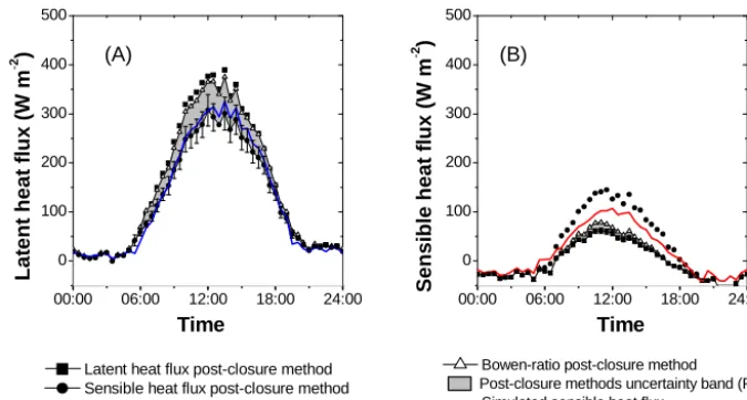
Figure 1. Illustration of the post-closure methods uncertainty band (PUB) to consider the systematic error in eddy covariance (EC) flux data.
The grey band shows the PUB computed as the difference between Bowen ratio-adjusted and non-adjusted fluxes. The closed squares in
(a) indicate the latent heat (LE) post-closed fluxes, and the close circles in (b) show the sensible heat (H) post-closed data. The error bars indicate the random measurement error. In some cases, the error bars are smaller than the size of the symbol and therefore not visible. Note:
in the case of latent heat flux, raw data andH post-closed data are identical. In the case of sensible heat flux, LE post-closed data and raw
data are identical.
Table 1. Overview of possible bound combinations to construct the post-closure methods uncertainty band (PUB). The upper and lower
bound of the band are constructed from the difference between raw fluxes and fluxes adjusted by one of the three post-closure methods
(Bowen ratio (B), sensible heat (H), and latent heat (LE) method).
Bound Lower bound= PUB width > 0 Useful
combination measured flux combination
LE H LE H
1.H–LE y y y y y
2.H–B y n y y n
3. LE–B n y y y n
4. raw–LE y y y n n
5. raw–H y y n y n
6. raw–B y y y y y
Note: y, yes; n, no.
BisCO) and light-limited rate. Moreover, a nitrogen (N) re-duction factor ranging from zero to unity is included to con-sider N limitation. Receiving 168 kg N per hectare of fertil-izer over the season, the winter wheat stand on our EC site is not N-limited, and thus the N reduction factor was set to unity.
In the following we will demonstrate the application of the PUB approach by evaluating the performance of NOAH-MP simulations to reproduce the EC flux data from a winter wheat stand and compare the performance of the Jarvis and Ball–Berry schemes. The simulation starts on day of drilling (11 October 2010) and ends on 22 July 2011 (about 1 week before final harvest at maturity). The soil profile was divided into four layers (0–0.1, 0.1–0.4, 0.4–1.0, and 1.0–2.0 m). The initial soil temperatures of the four layers were 285, 283, 282,
and 282 K. The initial soil water content was set to 24, 30, 41, and 43 vol. %. We used the USGS land use data set, vegeta-tion type index was set to 2 (dryland cropland and pasture), and soil type index was 8 (silty clay loam). The multi-physics options used in the simulation are listed in Table 2. Among other options, we selected a predefined monthly LAI and fractional vegetated area (FVEG) data. Monthly (green) LAI were linearly derived from measured total LAI data (Fig. 2). From mid-June until mid-July we assumed that the green LAI declined linearly from 4.6 to
[image:5.612.128.466.66.247.2] [image:5.612.163.431.379.495.2]Table 2. Setting of the multi-physics options used in the NOAH-MP simulation.
Multi-physics option Setting
Vegetation model opt_dveg=1: LAI and FVEG pre-defined in look-up table
Canopy stomatal resistance scheme opt_crs=1 or 2: Ball–Berry (1) or Jarvis (2) scheme
Runoff and groundwater model opt_btr=1: TOPMODEL-based simple groundwater model
Sensible heat exchange coefficient opt_sfc=1: Based on Monin–Obukhov similarity theory
Supercooled liquid water opt_frz=1: General form of the of the freezing-point depression equation (NY06)
Radiation transfer scheme opt_rad=3: Gaps=1−FVEG
Lower boundary of soil temperature opt_tbot=2: Constant temperature
Snow/soil temperature time scheme opt_stc=1: Semi-implicit
LAI: (green) leaf area index; FVEG: fractional vegetated area.
11 Nov 23 Dec 3 Feb 17 Mar 28 Apr 9 Jun 21 Jul
0 1 2 3 4 5
0.0 0.2 0.4 0.6 0.8 1.0
Green leaf area index Total leaf area index
L
e
a
f
a
re
a
i
n
d
e
x
(
m
2 m -2)
Date Fractional vegetated area
F
ra
c
ti
o
n
a
l
v
e
g
e
ta
te
d
a
re
a
(
1
[image:6.612.323.528.233.375.2])
Figure 2. Prescribed dynamics of the green and total leaf area index
and the fractional vegetated area used in NOAH-MP simulations. Note: until 15 June green and total leaf area index are the same.
3 Results and discussion
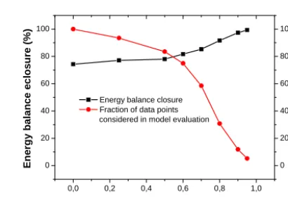
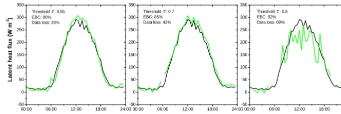
One of the first steps in constructing the PUB is to setτ (see Eq. 5). The choice of τ is a trade-off between the average EBR, i.e. the width of the PUB, and the number of data points remaining in the data set for model evaluation (Fig. 3). In our data set, atτ=0 3186 (i.e. 100 %) half-hourly fluxes passed the quality filter, and the average EBR was 74 %. Increas-ing τ to 0.5 improved the EBR only slightly. Atτ =0.55, both lines cross, the EBR increases to 80 %, and 20 % of the fluxes are excluded from the data analysis. Increasing τ to 0.8 improves EBR considerably (to 92 %) but strongly de-creases the number of data points remaining in the data set. With this choice, 69 % of the fluxes would not be considered in model evaluation. As a consequence, the mean monthly diurnal cycle of the energy fluxes deviate markedly from that withτ=0 (Fig. 4). The diurnal cycle becomes less contin-uous and more scattered, and data gaps show up during the morning and evening hours. In the present study, as a com-promise between the width of PUB and data loss, we set τ
to 0.7. With this choice, the EBR reaches 85 %, which cor-responds well to the average EBR of EC FLUXNET data
0,0 0,2 0,4 0,6 0,8 1,0 0
20 40 60 80 100
0 20 40 60 80 100
F
ra
c
ti
o
n
of
da
ta
po
in
ts
(
%
)
Energy balance closure Fraction of data points considered in model evaluation
E
n
e
rg
y
b
a
la
n
c
e
H
c
lo
s
u
re
(
%
)
Energy balance ratio threshold τ
Figure 3. Effect of the energy balance ratio thresholdτon the en-ergy balance closure and the fraction of data points remaining in the data set for model evaluation.
(Stoy et al., 2013). The diurnal cycle of the energy fluxes is still similar to that withτ =0, and at 42 % the data loss is in an intermediate range.
[image:6.612.61.275.235.384.2]00:00 06:00 12:00 18:00 24:00 -50
0 50 100 150 200 250 300 350
00:00 06:00 12:00 18:00 24:00 -50
0 50 100 150 200 250 300 350
00:00 06:00 12:00 18:00 24:00 -50
0 50 100 150 200 250 300 350
Threshold τ : 0.8 EBC: 92% Data loss: 69% Threshold τ : 0.7
EBC: 85% Data loss: 42%
L
a
te
n
t
h
e
a
t
fl
u
x
(
W
m
-2)
Time
Threshold τ : 0.55 EBC: 80% Data loss: 20%
Time Time
Figure 4. Effect of the energy balance ratio thresholdτon the pattern of the mean diurnal cycle of measured latent heat fluxes in May 2011.
Only flux data with an energy balance ratio (EBR)τ< EBR < 2−τwere used to compute the mean diurnal course (green line). The black line
shows the mean diurnal course forτ=0 .
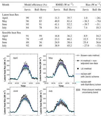
heat flux in the morning, but from noon to late afternoon both schemes, which produce very similar simulation re-sults, overestimate the latent heat flux. The above-mentioned findings can be underlined by the classical performance cri-teria (see Table 3). The modelling efficiency (EF) of the Jarvis scheme is highest in April. The root-mean-square er-ror (RMSE) is only 11.3 W m−2, and the simulation is nearly unbiased. In May and June both schemes deliver negatively biased latent heat fluxes. In July, the fluxes are positively bi-ased. Nevertheless, in all months the EF is high (78 to 99 %). With regard to the sensible heat flux, NOAH-MP tends to overestimate the flux during the main growth period of winter wheat (Fig. 6). Simulations based on the Ball–Berry scheme largely overestimate the sensible heat flux from April to June. The bias ranges from 34.2 to 57 W m−2, and in May the EF becomes negative (Table 3). Simulations based on the Jarvis scheme also overestimate the sensible heat flux but not as strongly as those based on the Ball–Berry scheme. The EF is always higher than with the Ball–Berry scheme, and, particularly in the afternoon hours of April, the simulations match the measured fluxes fairly well. In July, simulations with both schemes underestimate the sensible heat flux dur-ing most of the daytime (Jarvis: bias= −27.0 W m−2; Ball– Berry: bias= −33.6 W m−2).
In summary, the modeller would come to the conclusion that the default parameterization of NOAH-MP is not suited to simulate the surface energy fluxes at this winter wheat site. The Jarvis scheme outperforms the Ball–Berry scheme but also leads to strong systematic errors. From April to June, NOAH-MP overestimates the latent heat flux and underesti-mates the sensible heat flux. In July, the situation is opposite. In a next step, the modeller would try to improve the sim-ulations, e.g. by fine-tuning selected parameters within rea-sonable ranges. Ingwersen et al. (2011), for example, could distinctly improve NOAH simulations by replacing the de-fault constantrs,minwith fitted monthlyrs,minvalues. In the case of the Ball–Berry scheme an optimization of the empir-ical parameterm(see Eq. 7) would most probably bring the observed and simulated fluxes into closer agreement. A
fur-ther option is to search for multi-physics combinations that, with their default parameterization, lead to the best match of simulated and measured fluxes (Gayler et al., 2014).
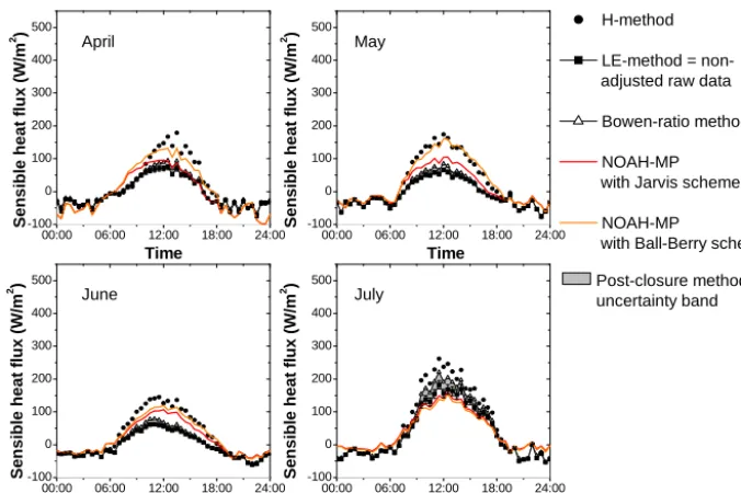
Figures 7 to 10 show the same simulation results as above but now with the proposed PUB. First, we discuss the re-sults based on the Bowen ratio PUB (Figs. 7 and 8). Over the daytime, the width of the PUB of the latent heat flux is on av-erage 49.7, 59.0, 47.7, and 29.5 W m−2in April, May, June, and July, respectively. The maximum width of the PUB is 88.0 W m−2 (17 % of net radiation) during noon in May. In May and June, latent heat fluxes simulated with the Jarvis scheme are well covered by the PUB (Table 4). In April, BC is only 35 %, and the Jarvis scheme has an upper bound pref-erence (BP=0.95, Table 4); in May and June its preference changes to the lower bound (BP= −0.29 in May and−0.49 in June). The Ball–Berry scheme has a good BC in April, and a BP of−0.53 indicates that the simulation is on aver-age enclosed by the PUB. In May and June, the BC is poor and the BP becomes smaller than−1, pointing to a system-atic underestimation of the latent heat flux though the fluxes are still in the range of the error bars. In July, the BC is low in both schemes, and in the early morning and afternoon the simulated fluxes are outside the PUB, with a BP markedly larger than unity pointing to a deficiency in the model.
[image:7.612.125.467.66.180.2]00:00 06:00 12:00 18:00 24:00 0 100 200 300 400 500
00:00 06:00 12:00 18:00 24:00 0 100 200 300 400 500
00:00 06:00 12:00 18:00 24:00 0 100 200 300 400 500
00:00 06:00 12:00 18:00 24:00 0 100 200 300 400 500
EC flux data (Bowen-ratio method)
NOAH-MP with Jarvis scheme
NOAH-MP
[image:8.612.129.468.79.303.2]with Ball-Berry scheme April L a te n t h e a t fl u x ( W m -2 ) Time L a te n t h e a t fl u x ( W m -2 ) Time May L a te n t h e a t fl u x ( W m -2 ) Time June L a te n t h e a t fl u x ( W m -2 ) Time July
Figure 5. State-of-the art approach to compare simulated and measured eddy covariance (EC) flux data. The monthly average cycles of
latent heat flux were computed based on Bowen ratio post-closed data. For modelling, the NOAH-MP land surface model was used in two configurations. The stomatal resistance was computed either with the empirical Jarvis scheme or the photosynthesis-based Ball–Berry scheme. The simulated fluxes are compared with measured EC flux data that were adjusted with the Bowen ratio method. The error bars indicate the random measurement error. In some cases, the error bars are smaller than the size of the symbol and therefore not visible.
00:00 06:00 12:00 18:00 24:00 -100 0 100 200 300 400 500
00:00 06:00 12:00 18:00 24:00 -100 0 100 200 300 400 500
00:00 06:00 12:00 18:00 24:00 -100 0 100 200 300 400 500
00:00 06:00 12:00 18:00 24:00 -100 0 100 200 300 400 500 April S e n s ib le h e a t fl u x ( W m -2 ) Time
EC flux data (Bowen-ratio method)
NOAH-MP with Jarvis scheme
NOAH-MP
with Ball-Berry scheme
S e n s ib le h e a t fl u x ( W m ) -2 Time May S e n s ib le h e a t fl u x ( W m -2 ) Time June S e n s ib le h e a t fl u x ( W m -2 ) Time July
Figure 6. State-of-the art approach to compare simulated and measured eddy covariance flux data. The monthly average cycles of sensible
[image:8.612.130.469.410.638.2]Table 3. Model performance criteria for the simulation results presented in Figs. 5 and 6. For the computation of model efficiency, root mean
square error (RMSE) and bias see, for example, Ingwersen et al. (2011). The performance criteria were computed for the daytime (06:00 to 18:00 UTC?).
Month Model efficiency (%) RMSE (W m−2) Bias (W m−2)
Jarvis Ball–Berry Jarvis Ball–Berry Jarvis Ball–Berry
Latent heat flux
April 99 93 11.3 35.7 1.0 −26.4
May 96 83 40.9 81.4 −36.3 −76.0
June 95 91 41.1 52.2 −39.7 −51.1
July 84 78 34.1 39.1 7.4 18.3
Sensible heat flux
April 91 59 16.8 36.2 8.9 34.2
May 78 −45 23.3 60.2 22.5 57.0
June 69 36 26.9 38.4 25.4 36.6
July 92 89 38.9 45.2 −27.0 −33.6
00:00 06:00 12:00 18:00 24:00 0
100 200 300 400 500
00:00 06:00 12:00 18:00 24:00 -100
0 100 200 300 400 500
00:00 06:00 12:00 18:00 24:00 0
100 200 300 400 500
00:00 06:00 12:00 18:00 24:00 0
100 200 300 400 500
Bowen-ratio method H-method = adjusted raw data
LE-method NOAH-MP with Jarvis scheme
NOAH-MP
with Ball-Berry scheme April
L
a
te
n
t
h
e
a
t
fl
u
x
(
W
m
-2 )
Time
Post-closure methods uncertainty band
L
a
te
n
t
h
e
a
t
fl
u
x
(
W
m
-2 )
Time May
L
a
te
n
t
h
e
a
t
fl
u
x
(
W
m
-2 )
Time
June
L
a
te
n
t
h
e
a
t
fl
u
x
(
W
m
-2 )
Time
July
Figure 7. Measured and simulated monthly average diurnal cycles of latent heat flux over a winter wheat stand in southwest Germany.
For modelling, the NOAH-MP land surface model was used in two configurations. The stomatal resistance was computed either with the empirical Jarvis scheme or the photosynthesis-based Ball–Berry scheme. The grey band shows the post-closure methods uncertainty band computed as the difference between the raw and Bowen ratio-adjusted fluxes. The error bars indicate the random measurement error. In some cases, the error bars are smaller than the size of the symbol and therefore not visible.
but now the BP becomes negative, and the measured sensi-ble heat fluxes are systematically underestimated from late morning to late afternoon.
As mentioned above, the Bowen ratio was low during the main growth period. Therefore, the H–LE method delivers for the latent heat flux very similar PUBs as the Bowen ratio method (Figs. 7 and 9). The width of the PUB of the LE-adjusted latent heat fluxes is somewhat higher than the fluxes adjusted with the Bowen ratio method and is on average 58.3, 68.7, 56.4, and 51.0 W m−2 in April, May, June, and July,
00:00 06:00 12:00 18:00 24:00 -100
0 100 200 300 400 500
00:00 06:00 12:00 18:00 24:00 -100
0 100 200 300 400 500
00:00 06:00 12:00 18:00 24:00 -100
0 100 200 300 400 500
00:00 06:00 12:00 18:00 24:00 -100
0 100 200 300 400 500 April
S
e
n
s
ib
le
h
e
a
t
fl
u
x
(
W
/m
2 )
Time
H-method
LE-method = adjusted raw data
Bowen-ratio method
NOAH-MP with Jarvis scheme
NOAH-MP
with Ball-Berry scheme
Post-closure methods uncertainty band
S
e
n
s
ib
le
h
e
a
t
fl
u
x
(
W
/m
2 )
Time May
S
e
n
s
ib
le
h
e
a
t
fl
u
x
(
W
/m
2 )
Time June
S
e
n
s
ib
le
h
e
a
t
fl
u
x
(
W
/m
2 )
[image:10.612.130.468.64.289.2]Time July
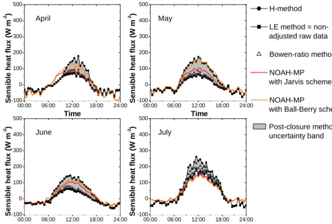
Figure 8. Measured and simulated monthly average diurnal cycles of sensible heat flux over a winter wheat stand in southwest Germany.
For modelling, the NOAH-MP land surface model was used in two configurations. The stomatal resistance was computed either with the empirical Jarvis scheme or the photosynthesis-based Ball–Berry scheme. The grey band shows the post-closure methods uncertainty band computed as the difference between the raw and Bowen ratio-adjusted fluxes. The error bars indicate the random measurement error. In some cases, the error bars are smaller than the size of the symbol and therefore not visible.
Table 4. Evaluation criteria of the Bowen ratio post-closure methods uncertainty bands presented in Figs. 7 and 8.
Month Band coverage (%) Bound preference (1)
Jarvis Ball–Berry Jarvis Ball–Berry
Latent heat flux
April 35 70 0.95 −0.53
May 74 4 −0.29 −1.67
June 67 33 −0.49 −1.15
July 7 7 1.96 2.67
Sensible heat flux
April 31 0 1.48 6.87
May 0 0 4.77 11.38
June 0 0 6.37 8.31
July 5 5 −2.26 −2.81
to 18:00, simulations with both schemes are fairly well cov-ered by the PUB. The Jarvis scheme results in a lower bound preference (BP= −0.71), whereas the Ball–Berry scheme has an upper bound preference (BP=0.53). In May, the sim-ulated fluxes based on the Jarvis scheme have a BC of 100 %. The BC of the Ball–Berry scheme is 67 %. Until 14:00 the simulated fluxes are close to the upper bound but still within the band. After 14:00 the sensible heat fluxes move above the upper bound, indicating a systematic overestimation during that period. In June, the BC is high with both schemes. While the fluxes simulated with the Jarvis are midway between both bands, those simulated with the Ball–Berry scheme have an
upper bound preference. In July, again simulations with both schemes underestimate the sensible heat flux and are outside the PUB. The BP falls out of the range of−1 to 1, pointing again to a model deficiency.
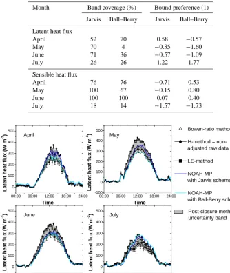
[image:10.612.166.429.394.550.2]jus-Table 5. Evaluation criteria of the post-closure methods uncertainty bands (PUBs) presented in Figs. 9 and 10. The PUB was computed from
the difference between sensible heat (H)- and latent heat (LE)-adjusted fluxes.
Month Band coverage (%) Bound preference (1)
Jarvis Ball–Berry Jarvis Ball–Berry
Latent heat flux
April 52 70 0.58 −0.57
May 70 4 −0.35 −1.60
June 71 36 −0.57 −1.09
July 26 26 1.22 1.77
Sensible heat flux
April 76 76 −0.71 0.53
May 100 67 −0.15 0.80
June 100 100 0.07 0.40
July 18 14 −1.57 −1.73
00:00 06:00 12:00 18:00 24:00 0
100 200 300 400 500
00:00 06:00 12:00 18:00 24:00 -100
0 100 200 300 400 500
00:00 06:00 12:00 18:00 24:00 0
100 200 300 400 500
00:00 06:00 12:00 18:00 24:00 0
100 200 300 400 500
Bowen-ratio method
H-method = adjusted raw data
LE-method
NOAH-MP with Jarvis scheme
NOAH-MP
with Ball-Berry scheme April
L
a
te
n
t
h
e
a
t
fl
u
x
(
W
m
-2 )
Time
Post-closure methods uncertainty band
L
a
te
n
t
h
e
a
t
fl
u
x
(
W
m
-2 )
Time May
L
a
te
n
t
h
e
a
t
fl
u
x
(
W
m
-2 )
Time
June
L
a
te
n
t
h
e
a
t
fl
u
x
(
W
m
-2 )
Time
July
Figure 9. Measured and simulated monthly average diurnal cycles of latent heat flux over a winter wheat stand in southwest Germany.
For modelling, the NOAH-MP land surface model was used in two configurations. The stomatal resistance was computed either with the empirical Jarvis scheme or the photosynthesis-based Ball–Berry scheme. The grey band shows the post-closure methods uncertainty band
(PUB) computed as the difference between sensible heat (H)- and latent heat (LE)-adjusted fluxes. The error bars indicate the random
measurement error. In some cases, the error bars are smaller than the size of the symbol and therefore not visible.
tified, because most of the time the simulations of the latent heat flux are well enclosed by the Bowen ratio and theH– LE PUB. Regarding the sensible heat flux, the results are ambiguous. Based on the Bowen ratio PUB, it appears that simulations with both schemes largely overestimate the sen-sible heat flux from April to May. According to the H–LE PUB, however, the simulated fluxes are still in the range of the uncertainty originating from the unclosed energy balance of the EC flux data. What we can reliably state is that (1), in the early morning hours of April, simulations with both schemes overestimate the sensible heat flux; (2) in May, the
Ball–Berry scheme underestimates the latent heat flux, caus-ing the sensible heat flux to move above the upper bound of theH–LE PUB; and (3) both schemes show a systematic er-ror over the daytime in July.
[image:11.612.131.465.97.492.2]00:00 06:00 12:00 18:00 24:00 -100
0 100 200 300 400 500
00:00 06:00 12:00 18:00 24:00 -100
0 100 200 300 400 500
00:00 06:00 12:00 18:00 24:00 -100
0 100 200 300 400 500
00:00 06:00 12:00 18:00 24:00 -100
0 100 200 300 400 500 April
S
e
n
s
ib
le
h
e
a
t
fl
u
x
(
W
m
-2 )
Time
H-method
LE method = adjusted raw data
Bowen-ratio method
NOAH-MP with Jarvis scheme
NOAH-MP
with Ball-Berry scheme
Post-closure methods uncertainty band
S
e
n
s
ib
le
h
e
a
t
fl
u
x
(
W
m
-2 )
Time May
S
e
n
s
ib
le
h
e
a
t
fl
u
x
(
W
m
-2 )
Time June
S
e
n
s
ib
le
h
e
a
t
fl
u
x
(
W
m
-2 )
Time July
Figure 10. Measured and simulated monthly average diurnal cycles of sensible heat flux over a winter wheat stand in southwest Germany.
For modelling, the NOAH-MP land surface model was used in two configurations. The stomatal resistance was computed either with the empirical Jarvis scheme or the photosynthesis-based Ball–Berry scheme. The grey band shows the post-closure methods uncertainty band
(PUB) computed as the difference between sensible heat (H)- and latent heat (LE)-adjusted fluxes. The error bars indicate the random
measurement error. In some cases, the error bars are smaller than the size of the symbol and therefore not visible.
cover in April, the illumination of the ground surface is very heterogeneous. Some positions are shaded by leaves, while others are sunlit. For example, while from 08:00 to 21:00, the coefficient of variation (CV) of the soil heat flux mea-sured at 8 cm depth (N=3) was 40.2 % in April, in June, due to a more homogeneous ground coverage, the CV de-clined to 17.9 %. Therefore, the possibility that the measured soil heat fluxes were positively biased cannot be excluded. A positively biased soil heat flux reduces the available energy, results in a better closure of the energy balance, and narrows the PUB.
The systematic underestimation of the latent heat flux by Ball–Berry based simulations in May might be explained by a non-adequate parameterization of the Ball–Berry scheme in the case of winter wheat. The default value of the em-pirical parameter min Eq. 7, which relates transpiration to CO2flux, is 9, as for all non-needleleaf forest USGS land use types. Mo and Liu (2001) simulated evapotranspiration (ET) and photosynthesis of winter wheat in the North China Plain and tested, among other things, the Ball–Berry scheme. They used in their simulation forma value of 11. Repeating the simulation withm=11 (data not shown) results in a nearly perfect match in May between simulated and measured non-adjusted latent heat fluxes (EF=99 %), the BC of the latent heat flux increases from 4 to 41 %, the negative bias declines from−76 to−36 W m−2, overall the Jarvis and Ball–Berry simulations move together, and the simulated sensible heat fluxes are also covered by theH–LE PUB.
The systematic error in July results from the fact that NOAH-MP does not distinguish between green LAI and to-tal LAI, i.e. the sum of green living and dead senescent leaves. This makes it impossible to adequately describe the surface energy exchange from a ripening winter wheat field. In our parameterization we prescribed that the (green) LAI linearly declines from 4.6 to 0 from mid-June until har-vest. This ensures that the transpiration, as under real field conditions, continuously decreases. In the radiation transfer scheme, however, this linearly declining LAI produces the situation of more and more shortwave radiation being ab-sorbed by the ground instead of by the vegetation. Shortly before harvest, the vegetated area is treated like a bare area, which is in disagreement with the real situation in the field. Also, below a fully senescent winter wheat, the ground is still shaded to a large extent, because the total LAI is still high (LAI∼3). Implementing into NOAH-MP a green LAI that is used in the stomatal resistance scheme to computers and a total LAI that is applied in the radiation transfer scheme to compute the partitioning of shortwave radiation absorbed by ground and vegetation would most probably improve the simulation result in July.
[image:12.612.128.468.67.296.2]instru-mental noise was usually one order of magnitude lower than the stochastic error. Overall, the random error was about one order of magnitude lower than the post-closure method er-ror, pointing to the importance of considering this error in analysing EC flux data.
In the literature, a few studies compared Bowen ratio-adjusted EC fluxes against a second independent method for measuring the latent heat flux. This provides some ex-perimental indication of the robustness of the Bowen ratio method. Wohlfahrt et al. (2010) tested EC ET rates against independent estimates from micro-lysimeters at a temper-ate mountain grassland over two measurement campaigns. The authors come to recommend forcing the energy balance closure by adjusting for the average Bowen ratio, meaning that the energy balance is closed on a daily basis by divid-ing the measured half-hourlyHand LE by the daily Bowen ratio. This implies that the Bowen ratio is conserved on a daily basis, but not necessarily the energy balance on half-hourly basis. Scott (2010) compared ET rates obtained with the EC method against the watershed balance over a pe-riod of 5 years in semi-desert grassland and desert scrub-land catchments in the USA. The author concluded that the justification for forcing the closure using the Bowen ratio method was ambiguous. Nine out of the investigated 13 years showed the same or less disagreement between EC and wa-tershed ET when measured fluxes were not adjusted. Barr et al. (2000) compared EC flux measurements with ET data ob-tained with the piezometric weighting lysimeter method at a boreal mature aspen stand. Over a period of 20 months, cumulative piezometric ET was 808 mm. Due to the overall low energy balance gap (on average 10 %), the two applied post-closure methods did not yield distinctly different results. Without flux adjustment, the EC method yielded a cumula-tive ET of 760 mm. Applying the Bowen ratio post-closure method slightly overestimated ET but led overall to a better agreement with the lysimeter method. The Bowen ratio post-closure method increased measured ET to 836 mm. More un-ambiguous results were obtained by Schume et al. (2005) and Wilson et al. (2001). Compared to the two other studies de-scribed above, the EBC was distinctly lower (about 80 %). For a temperate mixed European beech–Norway spruce for-est canopy, Schume et al. (2005) found a perfect agreement between non-adjusted latent heat flux data and the soil water balance method. Forcing the energy balance closure with the Bowen ratio method resulted in an overestimation of ET by 16 %. For a mixed deciduous oak forest, Wilson et al. (2001) compared the EC method with the catchment water balance method. Based on the latter, the 5-year average annual ET was 582 mm. This value agreed very well with non-adjusted ET data measured by the EC technique (571 mm per year). The authors did not apply any method for post-closing the energy balance, and do not give data on the Bowen ratio, but it suffices to state that the energy balance gap corresponds to about 143 mm of vaporized water. Under the climatic condi-tions at the site they mention (annual rainfall 1333 mm;
an-nual ET about 580 mm), one can expect the Bowen ratio to be distinctly lower than unity during most of the year. In other words, the Bowen ratio method would assign most of the en-ergy balance gap to the latent heat flux. Hence, also at the study site of Wilson et al. (2001), applying the Bowen ratio method would have overestimated the annual ET. This short review shows that there exist experimental indications that under some conditions the Bowen ratio method, and a for-tiori the LE method, might tend to overcorrect the latent heat flux, which fits with our finding that both schemes showed a clear lower bound preference in May and June.
All three post-closure methods assign the energy residual to the latent and/or sensible heat flux. Such approaches as-sume that the available energy at the surface is measured ac-curately, which is certainly not the case in the real world. Kohsiek et al. (2007) estimated that the error in the net ra-diation measurement during the EBEX-2000 campaign was up to 25 W m−2. Moreover, in the calculation of the available energy, the canopy storage and energy consumption by pho-tosynthesis (gross primary productivity, GPP), among other things, are usually not considered, because they are not mea-sured with conventional EC systems. Canopy storage be-comes particularly important for tall vegetation, but it can also reach 20 W m2 at crop sites, in particular during the morning hours (Meyers and Hollinger, 2004). On a daily av-erage, however, this flux cancels out. Energy consumption by photosynthesis can approach fluxes of the same order of magnitude as canopy storage. For an irrigated cotton field, Oncley et al. (2007) computed for the energy consumption by photosynthesis a diurnal average value of 8 W m−2 with a half-hourly peak value of formidable 48 W m−2. Jacobs et al. (2008) calculated in their study all possible enthalpy changes, such as the soil heat storage, vegetation cover heat storage, dew water heat storage, air mass heat storage, and the photosynthesis energy flux for a grass land site. By do-ing so, they were able improve the EBR of the EC flux data from 84 to 96 %. Also, Leuning et al. (2012) postulated that the closure of the energy balance is possible at half-hourly timescales by paying careful attention to all sources of surement and data processing errors and by accurately mea-suring net radiation and every energy storage term needed to calculate the available energy. Therefore, accurate measure-ment and considering the minor fluxes and storage terms in the calculation of the available energy would certainly help in reducing the energy balance gap, thereby narrowing the PUB and reducing uncertainty.
Recently, Charuchittipan et al. (2014) proposed a further post-closure method. They suggested closing the energy bal-ance based on the buoyancy flux ratio. In this approach, the fraction of the residual attributed to the sensible heat flux de-pends on the relative contribution of the sensible heat flux to the buoyancy flux. In general, this approach assigns larger fractions of the residual to the sensible heat flux than the Bowen ratio method does. In the context of the PUB, H
be in between the Bowen ratio- andH-adjusted fluxes. The difference between Bowen and buoyancy flux ratio-adjusted fluxes depends strongly on the Bowen ratio. At very high Bowen ratios (> 10), both methods result in very similar adjustments. At lower Bowen ratios, however, the difference between both methods increases. At a measured Bowen ra-tio of 0.2 and an EBC of 80 %, for example, the Bowen rara-tio method would assign 17 % of the residual toH, while, based on the buoyancy flux ratio method, this fraction increases to 86 % (at 20◦C) and the Bowen ratio shifts to 0.44. It remains to be seen whether this novel approach will prove its worth in the future.
In the present paper, PUB was not used to provide formal uncertainties but rather as a qualitative tool to identify peri-ods during which the model definitely showed structural de-ficiencies. This right-or-wrong decision tool is quite coarse because it filters out only the most obvious failure periods. Beyond this, it should be possible to use PUB, for example, in model inversion. Here, the BC could be directly used as an objective function. One could either search in the parameter space for the set of parameters with the highest BC or search for sets of parameters above a prescribed BC threshold. In the latter case one would get a distribution of parameters. In the GLUE (generalized likelihood uncertainty estimation; Beven and Binley, 2014) approach, which is well established in hy-drology, the PUB could be used as a criterion to distinguish between behavioural and un-behavioural model runs. Model parameterizations below a prescribed BC may be regarded as non-behavioural and thus excluded from the further un-certainty analysis. Within the framework of a Bayesian ap-proach for parameter estimation (see e.g. Braakhekke et al., 2013), PUB could be used to constrain the likelihood func-tion needed to compute the joined probability density.
4 Conclusions
We must be aware of the fact that, with computational ad-justment of the measured fluxes, we might add a substan-tial bias to the observed data, no matter which post-closure method we choose. In our study, the difference between the post-closing methods was up to 110 W m−2. The possible er-ror introduced by the post-closure method is about one or-der of magnitude larger than the random measurement error. This underlines the need to critically assess and communi-cate the possible error in eddy covariance flux data result-ing from the missresult-ing energy balance closure. The proposed post-closure methods uncertainty band (PUB) approach is an effective way to achieve this. Working with only one post-closure method may result in serious misinterpretations in model–data comparisons. For narrowing the PUB, we ur-gently need more research on the true nature of the energy balance residual.
Acknowledgements. We gratefully acknowledge the financial
support from the German Research Foundation (DFG) as part of Research Unit 1695 “Agricultural Landscapes under Global Climate Change – Processes and Feedbacks on a Regional Scale”. We thank the farmers Mr Bosch senior and Mr Bosch junior for their cooperation and the two anonymous reviewers for their helpful and inspiring comments.
Edited by: T. Keenan
References
Alavi, N., Berg, A. A., Warland, J. S., Parkin, G., Verseghy, D., and Bartlett, P.: Evaluating the impact of assimilating soil moisture variability data on latent heat flux estimation in a land surface model, Can. Water Resour. J., 35, 157–172, 2010.
Baldocchi, D., Reichstein, M., Papale, D., Koteen, L., Vargas, R., Agarwal, D., and Cook, R.: The role of trace gas flux networks in the biogeosciences, Eos, 93, 217–218, 2012.
Barr, A. G., King, K. M., Gillespie, T. J., den Hartog, G., and Neu-mann, H. H.: A comparison of Bowen ratio and eddy correlation sensible and latent heat flux measurements above deciduous for-est, Bound.-Lay. Meteorol., 71, 21–41, 1994.
Barr, A. G., Kamp, G. V. D., Schmidt, R., and Black, T. A.: Mon-itoring the moisture balance of a boreal aspen forest using a deep groundwater piezometer, Agric. For. Meteorol., 102, 13– 24, 2000.
Beven, K. and Binley, A.: GLUE: 20 years on, Hydrol. Process. 28, 5987–5918, 2014.
Blanken, P. D., Black, T. A., Yang, P. C., Neumann, H. H., Nesic, Z., Staebler, R., Den Hartog, G., Novak, M. D., and Lee, X.: Energy balance and canopy conductance of a boreal aspen forest: Partitioning overstory and understory components, J. Geophys. Res.-Atmos., 102, 28915–28927, 1997.
Blyth, E., Gash, J., Lloyd, A., Pryor, M., Weedon, G. P., and Shut-tleworth, J.: Evaluating the JULES land surface model energy fluxes using FLUXNET data, J. Hydrometeorol., 11, 509–519, 2010.
Braakhekke, M. C., Wutzler, T., Beer, C., Kattge, J., Schrumpf, M., Ahrens, B., Schöning, I., Hoosbeek, M. R., Kruijt, B., Kabat, P., and Reichstein, M.: Modeling the vertical soil organic matter profile using Bayesian parameter estimation, Biogeosciences, 10, 399–420, doi:10.5194/bg-10-399-2013, 2013.
Carrer, D., Lafont, S., Roujean, J., Calvet, J., Meurey, C., Le Moigne, P., and Trigo, I. F.: Incoming solar and infrared radiation derived from METEOSAT: Impact on the modeled land water and energy budget over France, J. Hydrometeorol., 13, 504–520, 2012.
Charuchittipan, D., Babel, W., Mauder, M., Leps, J. P., and Foken, T. T.: Extension of the averaging time in eddy-covariance mea-surements and its effect on the energy balance closure, Bound.-Lay. Meteorol., 152, 303–327. 2014.
Chen, F. F. and Dudhia, J.: Coupling and advanced land surface-hydrology model with the Penn State-NCAR MM5 modeling system, Part I: Model implementation and sensitivity, Mon. Weather Rev., 129, 569–585, 2001.
P., Basara, J. B., and Blanken, P. D.: Description and evaluation of the characteristics of the NCAR high-resolution land data as-similation system, J. Appl. Meteorol. Clim., 46, 694–713, 2007. Dudhia, J.: A nonhydrostatic version of the Penn State-NCAR mesoscale model: Validation tests and simulation of an Atlantic cyclone and cold front, Mon. Weather Rev., 1493–1513, 1993. Falge, E., Reth, S., Brüggemann, N., Butterbach-Bahl, K.,
Gold-berg, V., Oltchev, A., Schaaf, S., Spindler, G., Stiller, B., Queck, R., Köstner, B., and Bernhofer, C.: Comparison of surface en-ergy exchange models with eddy flux data in forest and grassland ecosystems of Germany, Ecol. Model., 188, 174–216, 2005. Farquhar, G. D., von Caemmerer, S., and Berry, J. A.: A
biochem-ical model of photosynthetic CO2 assimilation in leaves of C3
species, Planta, 149, 78–90, 1980.
Foken, T. T.: Der Bayreuther Turbulenzknecht, Universität Bayreuth, 19 pp., 1999.
Foken, T. T.: The energy balance closure problem: An overview, Ecol. Appl., 18, 1351–1367, 2008.
Gayler, S., Wöhling, T., Grzeschik, M., Ingwersen, J., Wizemann, H., Warrach-Sagi, K., Högy, P., Attinger, S., Streck, T., and Wulfmeyer, V.: Incorporating dynamic root growth enhances the performance of Noah-MP at two contrasting winter wheat field sites, Water Resour. Res., 50, 1337–1356, 2014.
Gerken, T., Babel, W., Hoffmann, A., Biermann, T., Herzog, M., Friend, A. D., Li, M., Ma, Y., Foken, T., and Graf, H.-F.: Tur-bulent flux modelling with a simple 2-layer soil model and ex-trapolated surface temperature applied at Nam Co Lake basin on the Tibetan Plateau, Hydrol. Earth Syst. Sci., 16, 1095–1110, doi:10.5194/hess-16-1095-2012, 2012.
Gielen, B., Verbeeck, H., Neirynck, J., Sampson, D. A., Vermeiren, F., and Janssens, I. A.: Decadal water balance of a temperate Scots pine forest (Pinus sylvestris L.) based on measurements and modelling, Biogeosciences, 7, 1247–1261, doi:10.5194/bg-7-1247-2010, 2010.
Hayashi, M., Jackson, J. F., and Xu, L.: Application of the versatile soil moisture budget model to estimate evaporation from prairie grassland, Can. Water Resour. J., 35, 187–208, 2010.
Ingwersen, J., Steffens, K., Högy, P., Warrach-Sagi, K., Zhunus-bayeva, D., Poltoradnev, M., Gäbler, R., Wizemann, H., Fang-meier, A., Wulfmeyer, V., and Streck, T.: Comparison of Noah simulations with eddy covariance and soil water measurements at a winter wheat stand, Agric. For. Meteorol., 151, 345–355, 2011.
IUSS: Working Group WRB: World Reference Base for Soil Re-sources 2006, first update 2007, Rome, 148 pp., 2007.
Jacobs, A. F. G., Heusinkveld, B. G., and Holtslag, A. A. M.: To-wards closing the surface energy budget of a mid-latitude grass-land, Bound.-Lay. Meteorol., 126, 125-136, 2008.
Kohsiek, W., Liebethal, C., Foken, T., Vogt, R., Oncley, S. P., Bern-hofer, C., and Debruin, H. A. R.: The Energy Balance Experi-ment EBEX-2000, Part III: Behaviour and quality of the radia-tion measurements, Bound.-Lay. Meteorol., 123, 55–75, 2007. Leuning, R., van Gorsel, E., Massman, W. J., and Isaac, P. R.:
Re-flections on the surface energy imbalance problem, Agric. For. Meteorol., 156, 65–74, 2012.
LI-COR Inc.: EddyPro, 2012
Mauder, M. and Foken, T.: Impact of post-field data processing on eddy covariance flux estimates and energy balance closure, Me-teorol. Z., 15, 597–609, 2006.
Mauder, M. and Foken, T.: Documentation and Instruction Man-ual of the Eddy-Covariance Software Package TK3, Universität Bayreuth, Abteilung Mikrometeorologie, 60 pp., 2011.
Mauder, M., Cuntz, M., Drüe, C., Graf, A., Rebmann, C., Schmid, H. P., Schmidt, M., and Steinbrecher, R.: A strategy for quality and uncertainty assessment of long-term eddy-covariance mea-surements, Agric. For. Meteorol., 169, 122–135, 2013.
Meyers, T. P. and Hollinger, S. E.: An assessment of storage terms in the surface energy balance of maize and soybean, Agric. For. Meteorol., 125, 105–115, 2004.
Mo, X. and Liu, S.: Simulating evapotranspiration and photosyn-thesis of winter wheat over the growing season, Agric. For. Me-teorol., 109, 203–222, 2001.
Moore, C. J.: Frequency response corrections for eddy correlation systems, Bound.-Lay. Meteorol., 37, 17–35, 1986.
Niu, G., Yang, Z., Mitchell, K. E., Chen, F., Ek, M. B., Barlage, M., Kumar, A., Manning, K., Niyogi, D., Rosero, E., Tewari, M., and Xia, Y.: The community Noah land surface model with multiparameterization options (Noah-MP): 1. Model description and evaluation with local-scale measurements, J. Geophys. Res.-Atmos., 116, 1–19, 2011.
Oncley, S. P., Foken, T., Vogt, R., Kohsiek, W., DeBruin, H. A. R., Bernhofer, C., Christen, A., van Gorsel, E., Grantz, D., Feigen-winter, C., Lehner, I., Liebethal, C., Liu, H., Mauder, M., Pitacco, A., Ribeiro, L., and Weidinger, T.: The energy balance experi-ment EBEX-2000, Part I: Overview and energy balance, Bound.-Lay. Meteorol., 123, 1–28, 2007.
Schotanus, P., Nieuwstadt, F. T. M., and DeBruin, H. A. R.: Tem-perature measurement with a sonic anemometer and its applica-tion to heat and moisture fluctuaapplica-tions., Bound.-Lay. Meteorol., 26, 81–93, 1983.
Schume, H., Hager, H., and Jost, G.: Water and energy exchange above a mixed European Beech – Norway Spruce forest canopy: A comparison of eddy covariance against soil water depletion measurement, Theor. Appl. Climatol., 81, 87–100, 2005. Scott, R. L.: Using watershed water balance to evaluate the accuracy
of eddy covariance evaporation measurements for three semiarid ecosystems, Agric. For. Meteorol., 150, 219–225, 2010. Skamarock, W. C., Klemp, J. B., Dudhia, J., Gill, D. O., Barker, D.
M., Duda, M. G., Huang, X. Y., Wang, W., and Powers, J. G.: A description of the Advanced Research WRF Version 3, 125 pp., 2008.
Spank, U., Schwärzel, K., Renner, M., Moderow, U., and Bernhofer, C.: Effects of measurement uncertainties of meteorological data on estimates of site water balance components, J. Hydrol., 492, 176–189. 2013.
Staudt, K., Falge, E., Pyles, R. D., Paw U, K. T., and Fo-ken, T.: Sensitivity and predictive uncertainty of the ACASA model at a spruce forest site, Biogeosciences, 7, 3685–3705, doi:10.5194/bg-7-3685-2010, 2010.
Twine, T. E., Kustas, W. P., Norman, J. M., Cook, D. R., Houser, P. R., Meyers, T. P., Prueger, J. H., Starks, P. J., and Wesely, M. L.: Correcting eddy-covariance flux underestimates over a grassland, Agric. For. Meteorol., 103, 279–300, 2000.
Webb, E. K., Pearman, G. I., and Leuning, R.: Correction of the flux measurements for density effects due to heat and water vapour transfer, Q. J. R. Meteorolog. Soc., 106, 85–100, 1980.
Wilson, K. B., Hanson, P. J., Mulholland, P. J., Baldocchi, D. D., and Wullschleger, S. D.: A comparison of methods for deter-mining forest evapotranspiration and its components: Sap-flow, soil water budget, eddy covariance and catchment water balance, Agric. For. Meteorol., 106, 153–168, 2001.
Wilson, K. K., Goldstein, A., Falge, E., Aubinet, M., Baldocchi, D., Berbigier, P., Bernhofer, C., Ceulemans, R., Dolman, H., Field, C., Grelle, A., Ibrom, A., Law, B. E., Kowalski, A., Meyers, T., Moncrieff, J., Monson, R., Oechel, W., Tenhunen, J., Valentini, R., and Verma, S.: Energy balance closure at FLUXNET sites, Agric. For. Meteorol., 113, 223–243, 2002.
Winter, J. M. and Eltahir, E. A. B.: The sensitivity of latent heat flux to changes in the radiative forcing: A framework for comparing models and observations, J. Clim., 23, 2345–2356, 2010. Wohlfahrt, G., Irschick, C., Thalinger, B., Hortnagl, L., Obojes, N.„